Role of slip between a probe particle and a gel in microrheology
Abstract
In the technique of microrheology, macroscopic rheological parameters as well as information about local structure are deduced from the behavior of microscopic probe particles under thermal or active forcing. Microrheology requires knowledge of the relation between macroscopic parameters and the force felt by a particle in response to displacements. We investigate this response function for a spherical particle using the two-fluid model, in which the gel is represented by a polymer network coupled to a surrounding solvent via a drag force. We obtain an analytic solution for the response function in the limit of small volume fraction of the polymer network, and neglecting inertial effects. We use no-slip boundary conditions for the solvent at the surface of the sphere. The boundary condition for the network at the surface of the sphere is a kinetic friction law, for which the tangential stress of the network is proportional to relative velocity of the network and the sphere. This boundary condition encompasses both no-slip and frictionless boundary conditions as limits. Far from the sphere there is no relative motion between the solvent and network due to the coupling between them. However, the different boundary conditions on the solvent and network tend to produce different far-field motions. We show that the far field motion and the force on the sphere are controlled by the solvent boundary conditions at high frequency and by the network boundary conditions at low frequency. At low frequencies compression of the network can also affect the force on the sphere. We find the crossover frequencies at which the effects of sliding of the sphere past the polymer network and compression of the gel become important. The effects of sliding alone can lead to an underestimation of moduli by up to 33%, while the effects of compression alone can lead to an underestimation of moduli by up to 20%, and the effects of sliding and compression combined can lead to an underestimation of moduli by up to 43%.
pacs
83.10.-y, 82.70.Gg, 83.50.Lh, 83.60.BcSingle particle microrheology [1, 2] has been a useful tool for measuring the material characteristics in situations where traditional rheometers are difficult to use. For example, it has been particularly useful in obtaining rheological measurements when large sample sizes are difficult to obtain, and when removing samples from their natural environment may be undesirable, such as in living cells. Traditional rheological measurements typically obtain the frequency-dependent macroscopic shear modulus , which relates shear stresses to homogeneous shear deformations. To interpret the results of single particle microrheological measurements, one must know what the response of a particle embedded in the material of question will be to driving forces (or equivalently, the force exerted on the particle in response to particle displacements). In practice, the response of such a particle has been assumed to relate to the macroscopic shear modulus via
| (1) |
when the particle with radius oscillates at frequency and displacement . The modulus is in general complex. In microrheological experiments, the use of this force response in conjunction with the fluctuation-dissipation theorem has been called the “generalized Stokes-Einstein relation”[1].
Eq. 1 holds true when the material may treated using continuum mechanics as a single incompressible phase with a complex shear modulus and no-slip boundary conditions between the particle and the material [2, 3]. The generalized Stokes-Einstein relation has been validated experimentally in the test case of a solution of wormlike micelles [4], but in many cases there are a number of issues that can complicate microrheological measurements, including compressional effects [2, 5], local depletion of the polymer [6, 7], modification of local properties via surface chemistry of the particles [8, 9], and violation of no-slip boundary conditions [10].
Although the technique of 2-particle microrheology [6, 11] ameliorates many of these problems, it is much more technically demanding than single-particle microrheology. Furthermore, fully understanding how all the above effects can impact 1-particle microrheology allows us to use it to understand materials and processes in which local heterogeneity plays an important role. In this paper we demonstrate how to quantify the effects arising from violation of the no-slip boundary condition for both an incompressible and compressible gel. Previous studies have treated the response of the medium to a particle in the case of no-slip boundary conditions [3, 2, 5, 12] and in the presence of compression [5]. In this work we include the effects of sliding between the sphere and the medium in a two-fluid model for a gel with phases representing a viscoelastic polymer network and fluid solvent. Throughout this paper, we work in the dilute network limit, which is appropriate for many microrheological studies, such as those of actin networks [5] and DNA solutions [7]. Sliding is implemented using a kinetic friction law—the shear stress of the network is proportional to the relative velocity between the network and the surface of the sphere, with proportionality constant . No-slip () and frictionless sliding () boundary conditions can be obtained as limiting cases.
Physically, we can see the effects of slip by comparing two different situations: a solid sphere of radius moving with velocity through a liquid of viscosity , and a clean bubble of radius moving through the same liquid. In the first case, there is no slip at the surface of the sphere, and the drag force is . In the second case, the drag on the bubble is smaller, . In the far field, the velocity field for the fluid flow for the bubble is also reduced by a factor of relative to flow for the solid sphere [13].
Our use of the two-fluid model for a gel allows us to include the effects of sliding via a boundary condition between the sphere and polymer network, even as the solvent retains no-slip boundary conditions. Because the fluid and network are coupled by drag, far from the sphere there is no relative motion between the network and the solvent. However, because the fluid and network have different boundary conditions, the far-field motion can have the character of that driven by no-slip boundary conditions, that driven by frictionless sliding boundary conditions, or somewhere in between. We find that the far-field motion is controlled by frequency. In the high frequency limit, the far-field solution has the properties of a deformation driven by no-slip boundary conditions. In this case, the solvent flow is the same as the flow around a sphere in a simple viscous fluid and no-slip boundary conditions, and the network is dragged along by the solvent. In the low frequency limit, the far-field solution has the properties of a deformation driven by frictionless sliding boundary conditions. The network displacement is the same as the displacement around a sphere in a simple elastic solid and frictionless boundary conditions, and the drag prevents the solvent from moving faster than the network.
Similarly, the force felt by the sphere interpolates between the limits provided by no-slip and frictionless sliding boundary conditions. The effects of sliding and compression can be described using three crossover frequencies. In the following, is the radius of the probe particle, is the mesh size of the polymer network, is the viscosity of the solvent, and are effective Lamé coefficients of the network (Eq. 2), and is the friction coefficient between the probe particle surface and the polymer network (Eq. 14).
- 1.
Associated with sliding, for , and for .
- 2.
Associated with sliding friction, .
- 3.
Associated with compression, .
The properties of the force can be summarized as
- (a)
At frequencies larger than , , and , the response force obeys Eq. 1, and moduli deduced using the generalized Stokes-Einstein relation match macroscopic measurements.
- (b)
At frequencies smaller than and , but larger than , effects from sliding are important, the response force is reduced, and moduli deduced using the generalized Stokes-Einstein relation underestimate by up to 33%.
- (c)
At frequencies smaller than , but larger than or , effects from compression are important, the response force is reduced, and moduli deduced using the generalized Stokes-Einstein relation underestimate by up to 20%.
- (d)
At frequencies smaller than , , and , effects from both sliding and compression are important, the response force is reduced, and moduli deduced using the generalized Stokes-Einstein relation underestimate by up to 43%.
- (e)
In real systems, and may be frequency dependent, and therefore so are . In light of the above, if at any point in an experiment , caution should be exercised in applying the generalized Stokes-Einstein relation. Our results provide a way to analyze microrheological data in this more complicated situation.
The paper is organized as follows. In Section I we introduce the two-fluid model for a gel and discuss how sliding boundary conditions can lead to qualitatively new behaviors. We discuss these behaviors in the simple geometry of a gel between two oscillating plates. In Section II we describe the analytic solution for the force exerted on an oscillating sphere in a gel, with some details relegated to Appendix A. Then we describe the properties of the force in Section III. All the features associated with sliding are present in the case of an incompressible network, which we discuss in the main body of the paper. In the discussion we describe the implications for microrheological experiments, providing examples of how our results can be used to help interpret microrheological data. Finally, in Appendix B we describe the properties of the force in the presence of both sliding and a compressible network for completeness.
I The importance of boundary conditions in the two-fluid model for a gel

We describe the gel as a polymer network with Lamé coefficients and , interspersed with fluid with viscosity (Fig. 1). In general, we assume that the network shear modulus is complex, and write . The polymer and fluid are coupled to each other by a friction coefficient [5, 14, 15]. We ignore any inertial contributions to the equations of motion:
| (2) | |||||
| (3) | |||||
| (4) |
Here is the displacement field of the polymer network and is the velocity field of the solvent. is the volume fraction of the polymer network, and Eq. 4 expresses the overall mass conservation of the gel. In the limit of small volume fraction, we can approximate Eq. 4 as the incompressibility of the solvent, . In Eqs. 2 and 3, the dot denotes a material time derivative; throughout this paper we replace this with a partial time derivative since we only consider small displacements and work with these equations only to linear order. To deduce the forces exerted by the gel, we use the stress tensors
| (5) | |||||
| (6) | |||||
| (7) |
It is important to note that the moduli are effective moduli for the network in the presence of the solvent including, for example, osmotic effects. In addition, and have implicit dependence on volume fraction since the network stiffness depends on the network density. For a typical microrheological experiment, we are interested in a dilute network, with mesh size much larger than the network filament diameter. For such a dilute network, , where is the mesh size of the network [5]. We note that Eqs. 2 and 3 are not restricted to the dilute network limit; for example, in a dense network, these equations reduce to the poroelastic equations if is negligible compared to the other stresses in the system [16].
This model has previously been used by Levine and Lubensky [5] to confirm that even with compressional effects, the force on a sphere obeys Eq. 1 for a range of frequencies. Above this range of frequencies inertial effects become important, while below this range of frequencies, the compressibility of the material can become important. So far, the effects of compressibility have not been observed [17].
In this work, we also use the two-fluid model, so we can incorporate the compressibility effects described above. We ignore inertial effects, which typically are not important at frequencies used in microrheological measurements. However, while previous results were obtained for no-slip boundary conditions, we obtain exact analytical results using boundary conditions which allow the sphere to slide with respect to the polymer network. Our boundary conditions encompass both the no-slip and frictionless sliding limits with respect to the polymer network.
Although Norris [12] and Oestreicher [3] have previously obtained analytic solutions for the response function of a sphere in a material with a single complex shear modulus for both no-slip and frictionless sliding boundary conditions, a crucial feature of the two-fluid model is that the boundary conditions for the fluid and the network can be different. This feature opens up the possibility that the far-field behavior can reflect either the fluid or the network boundary conditions, depending on the frequency of motion.
A simple demonstration of this frequency-dependent behavior can be seen in a gel between two oscillating plates located at (Fig. 2a). The plates oscillate with amplitude along the direction, with no-slip boundary conditions between the plates and the solvent, . First consider no-slip boundary conditions between the plates and the network, [5]. In this case there is no relative motion between the network and the solvent, and both undergo simple shear motion for all frequencies. Since the strain is homogeneous, the stress exerted on upper plate is by definition determined by the macroscopic shear modulus . Writing this stress as leads to
| (8) |
When the network can slip past the plate, the situation becomes more complicated, since the strain need not be homogeneous. For example, suppose there is frictionless sliding between the plates and the polymer network, so that the tangential stress on the network vanishes at the plates, . For simplicity assume is real (). Only the -components of the velocity and displacement fields are nonzero, and the solutions are
| (9) | |||||
| (10) |
In these equations we introduce the complex quantity which implies an associated length scale,
| (11) |
The penetration depth determines the thickness of the layer next to each plate where the solvent moves relative to the network. Friction suppresses relative motion beyond the penetration depth.
The velocity and displacement fields are plotted in Fig. 2b. To see the range of behavior that is possible, it is useful to consider limiting cases. First, suppose there is no coupling between the network and the solvent, . Then the network has zero displacement and the solvent has homogeneous oscillatory strain (similar to solid black lines, Fig. 2). Now suppose . At sufficiently high frequency, the penetration depth is small compared to , and there is no relative motion between the network and the solvent in most of the gel. Deep within the gel, the solvent has a constant strain rate and the network has a constant strain. The penetration depth determines the size of the boundary layers where the displacement changes from uniform strain to no strain to satisfy the condition of zero tangential stress at each plate. On the other hand, when the frequency is sufficiently low, is approximately the mesh size and we may still have if is big enough. In this case, again there is no relative motion between the solvent and the network deep in the gel, but now the deformation of the network is small. The penetration depth determines the thickness of the boundary layers at each plate where the velocity of the solvent rises from the small velocity of the network to the velocity of the plate.
To determine the crossover frequency that marks the transition between the high- and low-frequency behavior, it is convenient to plot the strain of the network at the midplane of the gel, , as a function of dimensionless frequency, (Fig. 2c) . At high frequency, we see that – the network is dragged along with the solvent and the motion in the interior of the gel is simple shear. At low frequency, – the deformation of the network and velocity of the solvent in the interior of the gel are small. Figure 2c shows the crossover for various values of the coupling . The scaling of the crossover frequency with can be deduced by examining the spacing of the curves in Fig 2c. For , the crossover frequency is approximately , with power law ; while for , the crossover frequency is approximately , with power law . Later we will see similar behavior of the crossover frequency as a function of for the spherical geometry.


When , we observe from Fig. 2c that the crossover frequency satisfies , and thus conclude that for near . Let us further suppose that . In this case we can understand the crossover frequency by examining force balance on the gel. As emphasized earlier, the solvent and network move together except in the boundary layers near the plates. The plates exert no direct force on the network, so any shear on the network results from the motion of the solvent dragging the network along in the boundary layer, and any stress from network shear in the interior is ultimately supported by the traction of the solvent at the plate. The forces can be estimated by approximating and with piecewise linear functions, as in Fig. 3. In the limit of zero Reynold’s number, there is force balance on any given layer of gel. Consider a layer bounded by the plate on one side, with width . At the plate, the traction is of magnitude , where is the displacement at distance from the plate. At the other side of the layer, the solvent and network stresses add up to approximately . Equating these two stresses determines . Using , we find that the normalized strain . For the normalized strain is approximately one, meaning that , while for the normalized strain decreases rapidly. Therefore, our force balance argument yields the same crossover frequency we identified from Fig. 2c. Physically, the traction due to the network shear is supported by the drag force between the network and solvent in the boundary layer of relative motion. The higher the frequency, the faster the relative motion, the more drag force, and the greater the network shear will be in the interior of the gel.
This crossover behavior also shows up in the stress exerted by the gel on the plates. Suppose the force on the plates is interpreted as a measurement of the macroscopic shear modulus. Again expressing the stress exerted on the upper plate as , we obtain
| (12) | |||
| (13) |
Due to the slip and relative motion, the gel does not undergo a homogeneous shear deformation, and need not be equal to .
At high frequencies, the network is pulled by drag to move like the uncoupled solvent, and (Fig. 4a), showing the response of an elastic solid being sheared between the plates. Below the crossover frequency, decreases rapidly, taking the character of a network with frictionless sliding boundary conditions, which does not exert stress on the plates. Similarly, at high frequencies, (Fig. 4b), showing the viscous response of a simple fluid with viscosity sheared between the two plates. In Fig. 4b, the quantity plotted is , which is proportional to an apparent viscosity of the medium. Below the crossover frequency and for , the apparent viscosity is enhanced. The profile of Fig. 3 explains this enhancement: at low frequencies, is nearly zero, and the solvent shear is approximately . Therefore the viscous stress on the plate is approximately . In the rest of this paper we describe analogous physics which arises in the spherical geometry, and discuss its ramifications for microrheological experiments.
II Solution for sphere moving in gel
Consider a sphere of radius surrounded by a gel. We solve for the flows and displacements in the frame of the sphere, using spherical coordinates . We consider a sphere oscillating along the direction () with amplitude .
In the frame of the sphere, the boundary conditions for the fluid and solid at are and . The boundary conditions at the surface of the sphere are
| (14) |
Here the dot denotes a time derivative, and is the stress tensor of the polymer network. The last condition allows the polymer network to slide past the surface of the sphere in the tangential direction, with a stress exerted proportional to the relative velocity. The magnitude of the force is controlled by the friction coefficient . For we obtain no-slip boundary conditions, while for we obtain frictionless sliding.
In dimensionless form, Eqs. 2-4 and Eq. 14 are
| (15) | |||||
| (16) |
| (17) |
where we measure lengths in units of , time in units of , and pressures and stresses in units of . The dimensionless parameters are , , , , and . As mentioned before, [5], where is the mesh size of the polymer network, so that . For convenience we keep the same notation for dimensionless fields as we used for dimensional fields.
Our method is an extension of the classic solution by Stokes of a sphere moving through a viscous fluid [13]. The velocity field is divergence-free and can be expressed in terms of a single stream function :
| (18) |
On the other hand, the polymer is compressible, so the displacement field has both a stream function for the divergence-free part (), and a potential function for the curl-free part ():
| (19) |
Taking the curl and divergence of the above equations, leads to
| (20) | |||||
| (21) | |||||
| (22) |
The solution for is written in the appendix, and involves three undetermined coefficients.
Diagonalizing the equations for and yields
| (23) |
where
| (24) |
and is a two-by-two matrix. The appendix contains expressions for the matrix and eigenvalues , which diagonalize the equations. The appendix also contains the solutions for and ; each involves three undetermined coefficients.
The nine undetermined coefficients are determined by imposing the boundary conditions at infinity and the sphere surface. In addition, one must demand that Eq. 15 is satisfied by the combination of stream and potential functions in Eq. 19. The conditions on the coefficients are displayed in the appendix and determine the velocity and displacement fields.
From the velocity and the displacement fields the (nondimensional) stresses and pressure of the polymer and fluid can be calculated:
| (25) | |||||
| (26) | |||||
| (27) |
The total stress tensor is
| (28) |
Integrating the stress tensor over the surface of the sphere yields the total force on the sphere, which is (in dimensionless form)
| (29) | |||||
| (30) | |||||
In these expressions, whenever a square root appears, the root with positive real part should be chosen. This expression is one of the main results of this paper. Although it is in analytic form, it is still unwieldy. In the next section we summarize its properties.
III Properties of response force
The dimensional response force is Eq. 30 multiplied by . If interpreted using the generalized Stokes-Einstein relation, this yields effective moduli
| (31) | |||||
| (32) |
If Eq. 1 holds, we would expect , and . In the following we will describe the response force in terms of the effective moduli. The descriptions in the following sections are obtained by analyzing the form of Eq. 30. To give clarity to the discussion, in all the plots we assume that and are frequency-independent.
To understand the properties of the response force when the particle can slide past the network, first we look at the limit of incompressible network, , which displays all of the effects due to sliding boundary conditions. Network compressibility (finite ) complicates the situation by adding additional features to the effective moduli. We leave a detailed description of the more complicated scenario with effects from both sliding and compressibility to the appendix, but summarize the results in the discussion.
III.1 Frictionless limit with incompressible network
To illustrate the effects of sliding when the network is incompressible, we concentrate on the case of frictionless sliding between the sphere and the polymer network, . When both the network and solvent are incompressible and have no-slip boundary conditions, there is no relative motion between the network and the solvent, and Eq. 1 holds [2]. In contrast, when the polymer network has frictionless boundary conditions at the surface of the sphere, the network and solvent move relative to each other near the sphere. This relative motion between the network and solvent leads to drag forces which tend to diminish the relative motion, so that far from the sphere the network and solvent move together. The far field solution can be either that of an incompressible material driven by no-slip boundary conditions, that of an incompressible material driven by frictionless boundary conditions, or somewhere in between. As in the example of a gel between two oscillating plates, at high frequencies, the solution driven by the velocities (the solvent, with no-slip boundary conditions) wins out, while at low frequencies the solution driven by displacements (the polymer network, with frictionless boundary conditions) wins out.
In the limit of frictionless sliding () and incompressibility () Eq. 30 reduces to
| (33) |
The low frequency limit is obtained when the first term in the brackets in the denominator dominates over the second term, and the high frequency limit is obtained in the opposite case. Therefore the crossover frequency satisfies . For (sphere larger than mesh size), , while for (mesh size larger than sphere), . The expression for in the introduction is written in terms of variables which can be easily controlled experimentally using the approximation , and hence applies when . Note that in these two limits, the form of the crossover is the same as in the case of the plates but with the length scale replaced by ; in particular the dependence on is the same as in the case of the oscillating plates, with power law and , respectively.
For frequencies , the modulus obeys Eq. 1, so that and . For , behaves as
| (34) | |||||
For the lowest frequencies, the real modulus , 67% of the value in Eq. 1. The behavior of as a function of frequency is plotted in Fig. 5.


Now we turn to the imaginary modulus . Eq. 1 predicts that . In the example of the plates, we assumed , and found an enhancement in the effective viscosity at low frequencies. In the case of a sphere there is a similar enhancement to the effective viscosity, but sliding also affects the estimation of .
First consider the case where the network shear modulus is purely real (). In this case, all dissipation arises from the viscous solvent and friction between the solvent and the polymer network. The behavior of with is shown in Fig. 6a, , an apparent viscosity. When , the apparent viscosity is . For frequencies , the apparent viscosity of the “solvent” contribution tends towards a plateau with enhanced viscosity . Physically, as in the case of the plates, the solvent moves more than the network in a layer near the sphere. A region of enhanced solvent shear and viscous drag is set up as the solvent reduces its motion relative to the network, until far away the solvent takes the same motion as the network. As in the case of the plates, the enhancement depends on as . In the inset to Fig. 6a we plot rescaled by its low frequency value, , to show that the crossover value is .
Now consider the case when the imaginary part of the network modulus () is nonzero. In addition to the contribution to described in the previous paragraph, there are also contributions from the network modulus . For , the leading contribution is , the result of Eq. 1. When , the leading contribution is , 66% of the high-frequency contribution. For a constant , at high frequencies the contribution proportional to dominates, while at low frequencies the contribution from dominates. In total, behaves as shown in Fig. 6b.
III.2 Incompressible network with intermediate friction
For any finite value of , there will be a crossover from behavior similar to at low frequencies to behavior similar to at high frequencies, as shown in Fig. 7. The crossover is set by the condition and occurs at . Because the no-slip limit of is , appears to crossover from a low frequency limit of to the high frequency limit at . Similar behavior is seen in the imaginary modulus .

IV Discussion
The main aim of this paper is to provide an understanding of how sliding between a probe particle and polymer network can affect the response function in a gel. Motivated by experimental data, Starrs and Bartlett [10] have previously suggested the possiblity of frictionless sliding boundary conditions being relevant in microrheological experiments. Our solution shows how this may come about, despite the fact that the liquid solvent always couples to probe particles with no-slip boundary conditions in continuum fluid mechanics. We find that, due to the coupling between the solvent and polymer network, in far-field, the solvent can move as if it is driven by sliding boundary conditions. Specifically, when the fluid and polymer network have different boundary conditions, at high frequencies this coupling tends to lock the network into the motion of the fluid, while at low frequencies the coupling locks the fluid into the motion of the network.
Our analytical solution for the force on a probe particle in response to oscillatory motion quantifies the effect of sliding. We have described the effects of sliding on the force felt by probe particles in terms of an effective modulus . For high enough frequencies, matches the amcroscopic shear modulus , while for low frequencies may underestimate . We have identified two crossover frequencies, one associated with sliding (), and one associated with friction (). For any finite amount of surface friction, when frequency is reduced below both and (), tends to underestimate moduli by 33%.
The description in the previous paragraph applies in the case of an incompressible network, as treated in the body of this paper. However, in real materials the compressibility of the network can lead to additional reductions in . These compressional effects complicate the behavior of as a function of frequency, but may be relevant in experimental situations, so we have described them in detail in Appendix B. Intuitively, a compressible network is softer than an incompressible network and should exert a smaller force on an oscillating sphere. Our analytic solution identifies a third crossover frequency associated with compressive effects (). This is the same crossover frequency identified earlier by other investigators [2, 5]. In terms of the effective modulus , the effects of compression and sliding together are as follows: For frequencies much greater than , , and , matches the macroscopic modulus . For frequencies such that , compressional effects reduce by up to 20%. For frequencies such that , sliding effects reduce by up to 33%. Finally, for the lowest frequencies, much less than , , and , both compressional and sliding effects reduce by up to 43% relative to .
For any specific experiment, our results describe how the appropriate effects of sliding on single-particle measurements should be accounted for. For example, if , which occurs for particles larger than the mesh size, then a good estimate for is given by . Therefore can be estimated in experimental measurements, allowing determination of whether it is possible for corrections to Eq. 1 from sliding effects to be important. In general, will be frequency dependent, and therefore so will . A simple test which follows from our analysis is that if throughout the range of experimental frequencies , then one can determine that sliding will not affect the effective moduli. In the following two paragraphs, we apply this test to two sets of experimental results reported in the literature.
Starrs and Bartlett [10] have observed a 2/3 reduction in single-particle moduli for frequencies above in polystyrene solutions. Using the solvent viscosity of decalin (), a trap spring constant of , and Fig. 6 and 7 of Ref. [10], can be estimated to be 0.3 – 0.6 for frequencies between and . To obtain for the semidilute polystyrene solution (concentration ), we use a bead size [10], and estimate the correlation length as [18], where [10] is the radius of gyration. We obtain the estimate . From these estimates we conclude that may be slightly greater than , but not by orders of magnitude. Therefore the effects of sliding may be important.
On the other hand, Buchanan et. al. [4] have reported that the generalized Stokes Einstein relation is accurate in wormlike micellar solutions. Using the solvent viscosity of water, and the moduli from Fig. 1 of Ref. [4], it can be estimated that is between and for frequencies where the one particle microrheology data is reported, and in most cases . Using a mesh lengthscale of and particle radius of , . Our calculation would then lead to the conclusion that for most of the data reported, and certainly for frequencies [for which is at least an order of magnitude greater than ], the effects of sliding should not be important. In this system, discrepancies from the generalized Stokes-Einstein relation due to sliding effects can only appear for frequencies below .
In the examples provided above, we have focused on estimating , rather than . However, if , sliding effects will not appear until . This dependence on friction may provide a way to test the predictions of our analysis by varying the surface chemistry of the probe particles [8].
While in most of this discussion we have focused on probe particles larger than the mesh size (), our results also apply when the probe particle is smaller than the mesh size (). In this case, can be large and may be more easily accessible to experiments. In addition, when probe particles are much smaller than mesh size, they may be more likely to not directly interact with the network, leading to small values of the friction coefficient and large values for . Our solution provides a framework to analyze experiments in this regime of small probe particle size.
Finally, an additional observation from the form of our results is that there is the possibility for features of the frequency dependence of moduli, including power laws, to be obscured or distorted in the vicinity of the crossover frequencies , , and . This suggests that caution may be in order near these crossover frequencies.
In the literature there has been much discussion of how probe-material interactions can affect one-particle microrheological measurements. For example, near a probe particle the polymer network can be depleted by steric hindrance. One effect of this depletion zone is to change local rheological properties, but another may be to increase the likelihood that the bead slides relative to the polymer network [10]. Our calculation takes into account the second effect but not the first. Quantitative comparison of to experiments may require treatment of both effects, as well as the effects from adhesion of probe surface to polymer networks [9].
Acknowledgements We thank C. Wolgemuth for helpful discussions. This work was supported in part by National Science Foundation grants DMS-0615919 (TRP) and CMMI-0825185 (VS), and a Solomon Faculty Research Grant from Brown University (VS). TRP thanks the Aspen Center for Physics, where some of this work was completed.
Appendix A Details of solution
The solution to the equation for the stream function can be obtained by using the axisymmetry of the solution, so that is independent of . In addition, due to the boundary conditions at infinity, must be proportional to . Using these conditions in Eq. 21, we find that the radial dependence of satisfies an ordinary differential equation. The solution to which results in finite displacements at infinity is
| (35) |
where , in which the root with positive real part is chosen.
To obtain Eq. 23 we need to find the matrix which diagonalizes the equations for the stream function,
| (36) |
In the above time derivatives have been evaluated with respect to the oscillatory function which multiplies all parts of the solutions. Explicitly, is
| (37) |
and the eigenvalues are , .
The solutions to and (Eq. 23) are found by a similar procedure as the solution to . and must be proportional to to satisfy the boundary conditions. The radial dependence obeys an ordinary differential equation, and the solutions which result in finite velocities and displacements at infinity are
| (38) | |||||
| (39) |
Again, the square roots denote the root with positive real part. Note that it would not be difficult to generalize this method of solution to incorporate the effects of inertial terms.
The boundary conditions Eq. 17 at yield four (linear) equations for the coefficients , since there both the velocity and displacement fields each have an and component.
Additional conditions on the coefficients arise from the boundary conditions for the displacement and velocity field at . Athough each have an and a component, the and component give identical equations for the coefficients , leaving only 2 independent conditions out of the four:
| (40) | |||||
| (41) |
In these equations the matrix elements of appear.
Eq. 15 has terms proportional to , , , and . The parts proportional to the exponentials are automatically satisfied by the general solutions in Eqs. 35 and 39. The terms proportional to and give nontrivial relations for the coefficients . The and component give identical equations for the coefficients, again leaving two independent conditions out of the four:
| (42) | |||||
| (43) |
However, note that the first of these (from ) is not independent from the equations arising from the boundary conditions at .
Together, these produce only seven linearly independent equations for the nine coefficients A-J, so solving them leaves two coefficients undetermined. However, these undetermined coefficients only appear when the stream and potential functions are considered independently of one another; in the physically meaningful combinations expressing the velocity and displacement field no undetermined coefficients remain. Since the solutions are not illuminating, we do not write them down.
Appendix B Properties of the response force with compressible network
In this appendix we describe the properties of the response force when effects from compressibility of the network are included. First we isolate the effects of compressibility by examining the case of no-slip boundary conditions between the sphere and the network. Then we include effects from sliding of the sphere past the network.
B.1 No-slip limit with compressible network
In this section we address the limit of no-slip between the sphere and the polymer, when is finite. Examining the form of the solutions, one can see that the stream function corresponding to the compressive motion of the network involves an exponential with length scale . The compressive motion dies off at longer scales due to the coupling to the incompressible fluid. Associated with these compressive effects is a crossover frequency set by the condition , or . The expression for in the introduction is written in terms of variables which can be easily controlled experimentally using the approximation , and hence applies when . For frequencies less than , compressive effects of the network are important, while for frequencies above , compressive effects of the network are not important. This crossover is the same as that identified in previous studies [2, 5].
For frequencies , the real part of the modulus tends to , in accord with the expectations of Eq. 1. For frequencies , the real modulus is diminished, and for very low frequencies tends to the value
| (44) |
Eq. 44 ranges from 80-100% of the high frequency limit . For an incompressible network () there is no reduction, while maximal reduction (20%) occurs for and . For (reasonable values for an actin network), the reduction is about 14%. In Fig. 8 the behavior of is plotted.


Now we turn to the imaginary part of the effective modulus . As in the incompressible case it is useful to analyze contribution with separately from the polymer network contribution. At high frequencies, for , , in agreement with Eq. 1. For frequencies below , crosses over to behavior in which
| (45) |
Note that as , . This behavior is plotted in Fig. 9a, which shows the quantity (an apparent viscosity), so that the high frequency regime appears as a constant, while the low frequency regime diverges as . The low frequency divergence of the apparent viscosity results from the fact that at low frequencies, the compressive length scale diverges, and so there is a larger and larger volume with appreciable relative motion between the solvent and network. The dissipation at low frequencies is increased by the friction between compressive modes of the polymer network and the incompressible solvent. To show that the crossover frequency is , in one of the insets we plot rescaled by its low frequency magnitude, .
Now consider the case when the imaginary part of the network modulus () is nonzero. In addition to the contribution to described in the previous paragraph, there are also contributions from the network modulus . For high frequencies (), this additional contribution is simply , as expected from Eq. 1. For low frequencies this contribution is diminished to the limiting value
| (46) |
As in the real part, the low frequency value is between 80% (for , ), and 100% (incompressible, ) of the high frequency value. For , at low frequencies the low frequency additional contribution is about 81% of the high frequency additional contribution.
For a constant , at high frequencies the contribution proportional to dominates, while at low frequencies the contribution from dominates. This yields which behave as shown in Fig. 9b and c. Note that the low frequency enhancement discussed in the case is not readily apparent since the contribution from dominates at low frequencies.
B.2 Frictionless limit with compressible network
Now we turn to the opposite limit of no friction between the polymer and sphere (). As in the incompressible case, we expect that for frequencies below the far-field solution takes the character of a solution with frictionless sliding boundary conditions. For frequencies , the modulus obeys Eq. 1, so that and . For frequencies less than , now that there is also compressibility, there are two cases to consider. In the first case, , while in the second case .
First, consider the case where . For , the real modulus , 66% of the value in Eq. 1. For , compressive effects come into play and further diminish , which tends to
| (47) |
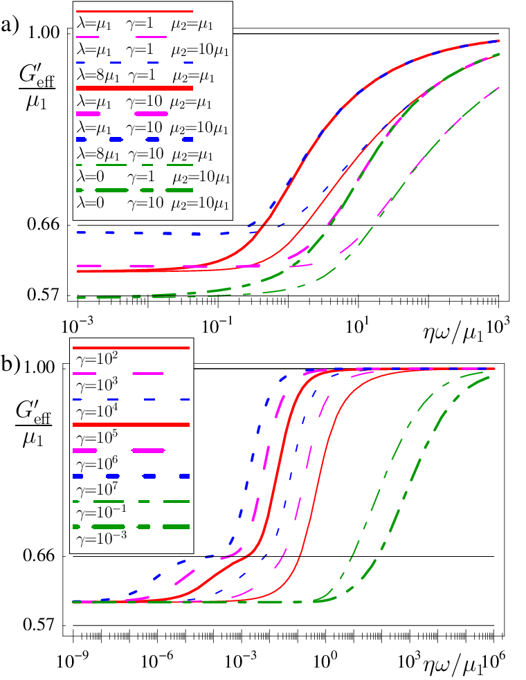
The low frequency limit of is between 57% (compressible limit with , ) and 66% (incompressible limit, ) of the high frequency value. For , the low frequency limit of is about 60% of the high frequency value .
In practice the condition that may not be met, either because , or because is not sufficiently smaller than . In this case appears to immediately tend to the behavior of Eq. 47 when . We plot representative behavior of in the frictionless limit in Fig. 10.

Now we turn to the imaginary modulus . Again, first look at the contribution arising from the solvent viscosity and drag between the polymer network and solvent, by setting . When , the imaginary modulus . For frequencies , crosses over to behavior of
| (48) |
The behavior of with is shown in Fig. 11a, which shows the apparent viscosity . In one of the insets we plot rescaled by its low frequency value, , to show that the crossover value is . Note that for certain parameters, as decreases, one can see the effective viscosity approach a plateau, which has the same origin as the plateau in the incompressible case described in the main text. At even lower frequencies, Eq. 48 is dominated by behavior. This has the same origins in the compressibility of the network as discussed in the previous section dealing with no-slip boundary conditions.
If there is an additional contribution to the imaginary modulus. For , this contribution is , the result of Eq. 1. When , this contribution is . Finally, when , this contribution tends to the limiting value
| (49) |
This limiting value is smaller than the contribution from at high frequencies. It is between 57% (compressible limit, , ), and 66% (incompressible limit, ) of the high frequency contribution corresponding to Eq. 1. For the limiting value is 58% of the high-frequency contribution.
If , for the additional contribution to immediately tends to the value in Eq. 49.
B.3 Intermediate friction
For any finite value of , there will be a crossover from behavior similar to at low frequencies to behavior similar to at high frequencies.
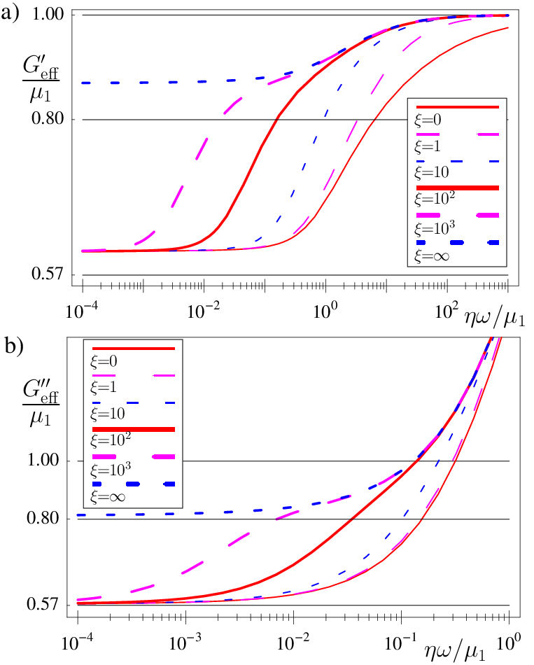
The crossover occurs at . Typically, as plotted in Fig. 12, because the no-slip limit of is closer to , appears to crossover from a low frequency limit of (or less, if compressional effects are important) to a value closer to the high frequency limit at . Similar behavior is seen in the imaginary modulus , shown in Fig. 12.
References
- [1] T. G. Mason and D. A. Weitz, Phys. Rev. Lett. 74, 1250 (1995).
- [2] B. Schnurr, F. Gittes, F. C. MacKintosh, and C. F. Schmidt, Macromolecules 30, 7781 (1997).
- [3] H. L. Oestreicher, J. Acoust. Soc. Am. 23, 707 (1951).
- [4] M. Buchanan, M. Atakhorrami, J. F. Palierne, and C. F. Schmidt, Macromolecules 38, 8840 (2005).
- [5] A. J. Levine and T. C. Lubensky, Phys. Rev. E 63, 041510 (2001).
- [6] J. C. Crocker, M. T. Valentine, E. R. Weeks, T. Gisler, P. D. Kaplan, A. G. Yodh, and D. A. Weitz, Phys. Rev. Lett. 85, 888 (2000).
- [7] D. T. Chen, E. R. Weeks, J. C. Crocker, M. F. Islam, R. Verma, J. Gruber, A. J. Levine, T. C. Lubensky, and A. G. Yodh, Phys. Rev. Lett. 90, 108301 (2003).
- [8] J. L. McGrath, J. H. Hartwig, and S. C. Kuo, Biophys. J. 79, 3258 (2000).
- [9] M. T. Valentine, Z. E. Perlman, M. L. Gardel, J. H. Shin, P. Matsudaira, T. J. Mitchison, and D. A. Weitz, Biophys. J. 86, 4004 (2004).
- [10] L. Starrs and P. Bartlett, Faraday Disc. 123, 323 (2003).
- [11] A. J. Levine and T. C. Lubensky, Phys. Rev. Lett 85, 1774 (2000).
- [12] A. N. Norris, J. Acoust. Soc. Am. 119, 2062 (2006).
- [13] G. K. Batchelor, An introduction to fluid mechanics (Cambridge University Press, Cambridge, 1967).
- [14] P. G. de Gennes, Macromolecules 9, 587 (1976).
- [15] S. T. Milner, Phys. Rev. E 48, 3674 (1993).
- [16] S. I. Barry and M. Holmes, IMA Journal of Applied Mathematics 66, 175 (2001).
- [17] F. C. MacKintosh and A. J. Levine, Phys. Rev. Lett 100, 018104 (2008).
- [18] F. Brochard and P. G. de Gennes, Macromolecules 10, 1157 (1977).