Finite Larmor radius effects on non-diffusive tracer transport in a zonal flow
Abstract
Finite Larmor radius (FLR) effects on non-diffusive transport in a prototypical zonal flow with drift waves are studied in the context of a simplified chaotic transport model. The model consists of a superposition of drift waves of the linearized Hasegawa-Mima equation and a zonal shear flow perpendicular to the density gradient. High frequency FLR effects are incorporated by gyroaveraging the velocity. Transport in the direction of the density gradient is negligible and we therefore focus on transport parallel to the zonal flows. A prescribed asymmetry produces strongly asymmetric non- Gaussian PDFs of particle displacements, with Lévy flights in one direction but not the other. For , where is the characteristic wavelength of the flow and is the thermal Larmor radius, a transition is observed in the scaling of the second moment of particle displacements, . The transition separates ballistic motion, , at intermediate times from super-diffusion, , at larger times. This change of scaling is accompanied by the transition of the PDF of particle displacements from algebraic decay to exponential decay. However, FLR effects seem to eliminate this transition. In all cases, the Lagrangian velocity autocorrelation function exhibits non-diffusive algebraic decay, , with to a good approximation. The PDFs of trapping and flight events show clear evidence of algebraic scaling with decay exponents depending on the value of . The shape and spatio-temporal self-similar anomalous scaling of the PDFs of particle displacements are reproduced accurately with a neutral, , asymmetric effective fractional diffusion model where and are the orders of the spatial and temporal fractional derivatives.
pacs
52.25.Gj,52.35.Kt,52.65.Cc,05.40.Fb,05.45.Pq,52.25.Fi,52.65.-yI Introduction
Plasma turbulence presents a challenge to multiscale models of transport in applications such as magnetic fusion confinement, stellar accretion disks and galactic dynamos. Simulations of turbulent transport involve nonlinear interactions at disparate scales, which often makes numerical computations expensive and analytic methods intractable. As an alternative, one may consider models of intermediate complexity that incorporate important aspects of transport within a relatively simple reduced description. In this paper we follow this approach and present a numerical study of the role of finite Larmor radius (FLR) effects on non-diffusive poloidal transport in zonal shear flows using a reduced Hamiltonian test particle transport model.
Following Ref. [1], we model the flow as a superposition of a shear flow and drift waves obtained from the linearized Hasegawa-Mima (HM) equation [2]. Test particle characteristics in this flow are generally not integrable and exhibit chaotic advection, also known as Lagrangian turbulence, which reproduces key ingredients of particle transport in more complex flows. High frequency FLR effects are incorporated by solving the test particle equations of motion for the gyroaveraged velocity. As demonstrated by Ref. [3], we compute the gyroaverage using a discrete -polygon approximation.
We adopt a statistical approach and apply non-diffusive transport diagnostics to large ensembles of particles. One of the simplest diagnostics is the scaling of the second moment of particle displacements, , where denotes the particle’s displacement and denotes the ensemble average. In the standard diffusion case, , linear scaling allows the definition of an effective diffusivity as the ratio in the limit of large . However, in the case of non-diffusive transport, with . When , the growth of the variance is slower than diffusion and transport is sub-diffusive. When transport is super- diffusive, which means the spreading is faster than diffusion, and the displacements may be Lévy flights [4]. In both super- and sub-diffusion, characterization of transport as a diffusive process with an“effective diffusivity” breaks down because when , and when . Other measures of non-diffusive transport, which will be discussed in detail later, include non-Gaussianity of the probability distribution of displacements (propagator), slow decay of the Lagrangian velocity autocorrelation function, the presence of long jumps (Lévy flights) and long waiting times, and the non-local (i.e., non-Fickian) dependence of fluxes on gradients. A general review of non-diffusive transport can be found in Ref. [5], and discussions focusing on plasmas can be found in Ref. [6, 7].
Test particle transport in HM flows, as in Fig. 1(a), has been studied in Refs. [8, 9, 10, 11, 12, 1, 13]. In Ref. [1], which did not include FLR effects, it was shown that zonal flows give rise to Lévy flights and strongly asymmetric non-Gaussian PDFs of particle displacements. References [9, 10] addressed the role of FLR effects but restricted attention to diffusive transport. More recently, Ref. [13] considered FLR effects in non-diffusive transport in HM turbulence and concluded that the exponent does not change appreciably with the Larmor radius but that the effective diffusion coefficient is reduced. There is a very close connection between drift waves as described by the HM equation and Rossby waves as described by the quasigeostrophic equation, see for example Ref. [14]. Therefore, statistical test particle studies in fluid mechanics, such as Refs. [15, 16], are in principle applicable to drift wave transport.

The main new results presented here, which to our knowledge have not been reported in the literature before, include: (i) a transition from algebraic to exponential decay in the tails of PDFs of particle displacements accompanied by a transition from ballistic () to super- diffusive () transport; (ii) a numerical study of the role of FLR on the Lagrangian velocity autocorrelation function and on the particle trapping and particle flight PDFs; (iii) the construction of a effective fractional diffusion model that reproduces the shape and the spatio-temporal anomalous self-similar scaling of the PDF of particle displacements. In recent years, fractional diffusion models have been applied to describe non-diffusive plasma transport, e.g. Refs. [17, 18, 19, 20, 21, 22]. Although the present work focuses on a prototypical model of transport, the diagnostics used and the non-diffusive phenomenology discussed here might be of relevance to the study of transport in more general flows dominated by coherent structures like zonal flows and eddies. Despite the fact that these coherent structures are ubiquitous in simulations and experiments [14, 23, 24], their influence on non-diffusive transport is not well understood. In this regard, Ref. [25] showed evidence of non-diffusive transport in gyrokinetic turbulence for “intermediate” simulation times.
The rest of the paper is organized as follows. In Sec. II the transport model with and without FLR effects is explained. Section III shows a benchmark of the numerical method against an exact solution for the particle propagator in a parallel flow. Section IV presents a summary of Lagrangian diagnostics to study non-diffusive transport. The main numerical results are presented in Sec. V. Section VI describes the anomalous self-similarity properties of the PDF of particle displacements and presents an effective fractional diffusion model. Section VII contains the conclusions.
II Transport model
We follow a Lagrangian approach to study transport and consider large ensembles of discrete particles moving in a prescribed flow. We limit attention to test particles, neglecting self-consistency effects and assuming that the particles are transported by the flow without modifying it. When finite Larmor radius (FLR) effects can also be neglected, the dynamics are determined by a drift equation which, in the approximation, is
| (1) |
where denotes the particle position, is the electrostatic field, and is the magnetic field. Writing , and , Eq. (1) can be equivalently written as the Hamiltonian dynamical system
| (2) |
where the electrostatic potential is analogous to the Hamiltonian, and the spatial coordinates are the canonical conjugate phase space variables.
For relatively high energy particles or for a flow varying relatively rapidly in space, the zero Larmor radius approximation fails and it is necessary to incorporate FLR effects. A simple, natural way of doing this is to substitute the flow on the right hand side of Eq. (2), which is evaluated at the location of the guiding center, by its value averaged over a ring of radius , where is the Larmor radius [3]. Formally, the procedure is given by
| (3) |
where the gyroaverage, , is defined as
| (4) |
This is a good approximation provided the gyrofrequency is greater than other frequencies in the system.
In the HM model for drift waves the electrostatic potential is determined from [2]
| (5) |
where the coordinate corresponds to the direction of the density gradient driving the drift-wave instability, and corresponds to the direction of propagation of the drift-waves. In toroidal geometry, is analogous to a normalized coordinate along the minor radius, and is a poloidal-like coordinate. Here we assume a slab approximation and treat as Cartesian coordinates. The parameter measures the scale length of the density gradient. We model the electrostatic potential (test particle Hamiltonian) as a superposition of an equilibrium zonal shear flow, , and the corresponding eigenmodes of Eq. (5), , with perpendicular wave numbers, , and frequencies, ,
| (6) |
We consider a monotonic zonal flow of the form
| (7) |
In this case, depending on the parameter values, there is a band of unstable modes bounded by two regular neutral modes with eigenfunctions [1]
| (8) |
Since these modes are neutral, and are real and the corresponding values of are obtained from the linear dispersion relation. Neutral modes are important because they describe dynamics near marginal stability. Following Ref. [1], we consider a traveling wave perturbation of the first neutral mode. The electrostatic potential in the co-moving reference frame of the neutral mode takes the form
| (9) |
The first term on the right hand side of Eq. (9) is the potential of the shear flow in Eq. (7), and is the frequency of the perturbation. The wavenumbers perpendicular to the uniform magnetic field, and , characterize the size of eddies, while and give the amplitudes of the waves. When computing to compare the scale length of the eddies in this flow to the thermal gyroradius, we use the mean value .
When the Hamiltonian in Eq. (9) is time independent, and the test particles follow contours of constant shown in Fig. 1(b). In this case, particles inside the separatrix remain trapped and those outside the separatrix are always untrapped with left of the vortices and right of the vortices. However, when there is a time dependent perturbation, i.e. when in Eq. (9), the particle trajectories are in general not integrable. In this case, the separatrix breaks and forms a stochastic layer where test particles alternate chaotically between being untrapped in the zonal flow and being trapped inside the vortices. This is the phenomenon of chaotic transport that has been studied in both plasmas and fluid systems, see for example Refs. [8, 26, 27, 15] and references therein. As Fig. 1(a) illustrates, the simple Hamiltonian model in Eq. (9) provides a reduced description of eddies embedded in a background zonal flow in HM turbulence.
III Numerical method
The zero Larmor radius calculations are based on the Hamitonian-like equations of Eq. (2). For the numerical integration of these equations we used the second-order symplectic predictor-corrector scheme of Ref. [28] with a fixed time step of 0.05 and 8 iterations in the predictor-corrector loop. These parameters were chosen based on numerical convergence studies and by monitoring the accuracy of energy conservation. For the model parameters we used , , , , and . This choice is motivated by Refs. [15, 1] where it was shown that, for this set of parameters, test particles exhibit strongly asymmetric, non-Gaussian statistics. As such, these parameters are a good starting point to study the role of FLR effects on non-diffusive transport. For the initial conditions we used an ensemble of particles located in the vicinity of the hyperbolic fixed point of the Hamiltonian at . This localization guarantees that a large fraction of the particles will stay in the stochastic layer and undergo chaotic transport. Other choices of initial positions can lead to integrable motion with particles permanently either inside the eddies, circling, or outside, following the zonal flow.
The only difference between the zero and finite Larmor radius calculations is in the evaluation of the velocity of the test particle. Assuming fast gyration in a strong field, the gyroaverage of the velocity is computed over a circle of radius , where is the Larmor radius of the particle. Throughout this paper we will assume a Maxwellian equilibrium distribution for the Larmor radii of the test particles of the form
| (10) |
normalized according to . For the numerical computation of the gyroaverage we approximate the circle with an inscribed polygon with -sides and approximate the integral over the circle as the average over the vertices of the polygon. This method, widely used in kinetic particle codes (e.g. [3]), simply samples the field on the gyration arc at a small number of equally spaced points. For example, the 8-point (octagon) approximation evaluates the gyroaverage by considering points distributed around the circle in equal increments, i.e., at . If the mean gyroradius, , becomes large relative to the typical scale length, , of the flow, i.e., if , the number of points used to compute the gyroaverage must be increased to maintain the same level of accuracy.
The error involved in the approximation of the gyroaverage on for a given value of and, therefore, a benchmark for the accuracy of the numerical scheme can be studied by considering the following parallel flow in arbitrary geometry
| (11) |
The main object of interest is the probability distribution function of particle displacements, or propagator, , which gives the probability for a particle to be at at time if it was at at time . Since for this choice of , we restrict study to the direction. The function depends on and the goal is to study the error in the numerical evaluation of as function of and the value of used in the approximation of the gyroaverage. As discussed in Appendix A, the exact propagator for Eq. (11) is given by
| (12) |
with
| (13) |
where denotes the i-th zero of the equation . Here, is the order zero Bessel function of the first kind. For a given , the number of zeros of this equation is which goes to as goes to zero. Note also that because the minimum and maximum values of are and , respectively, no zero exists for or . Therefore, identically vanishes outside the interval . Despite its apparent complexity, this analytical result provides a valuable benchmark to assess the accuracy of the gyroaverage computation.
Figure 2 compares the exact propagator in Eq. (12) with the propagator obtained from direct numerical integration of the gyroaverage equations of motion in Eq. (3) for different values of and . The FLR effects significantly change the propagator, which is a -function centered at : . It is observed that for , produces relatively good results, although it misses the small spike in around . Other cases with (not shown) give nearly exact agreement. However, for , the average departs significantly from the exact result. This failure means that choosing , such as , is necessary. One is led to conclude that the method should not be used for values of .
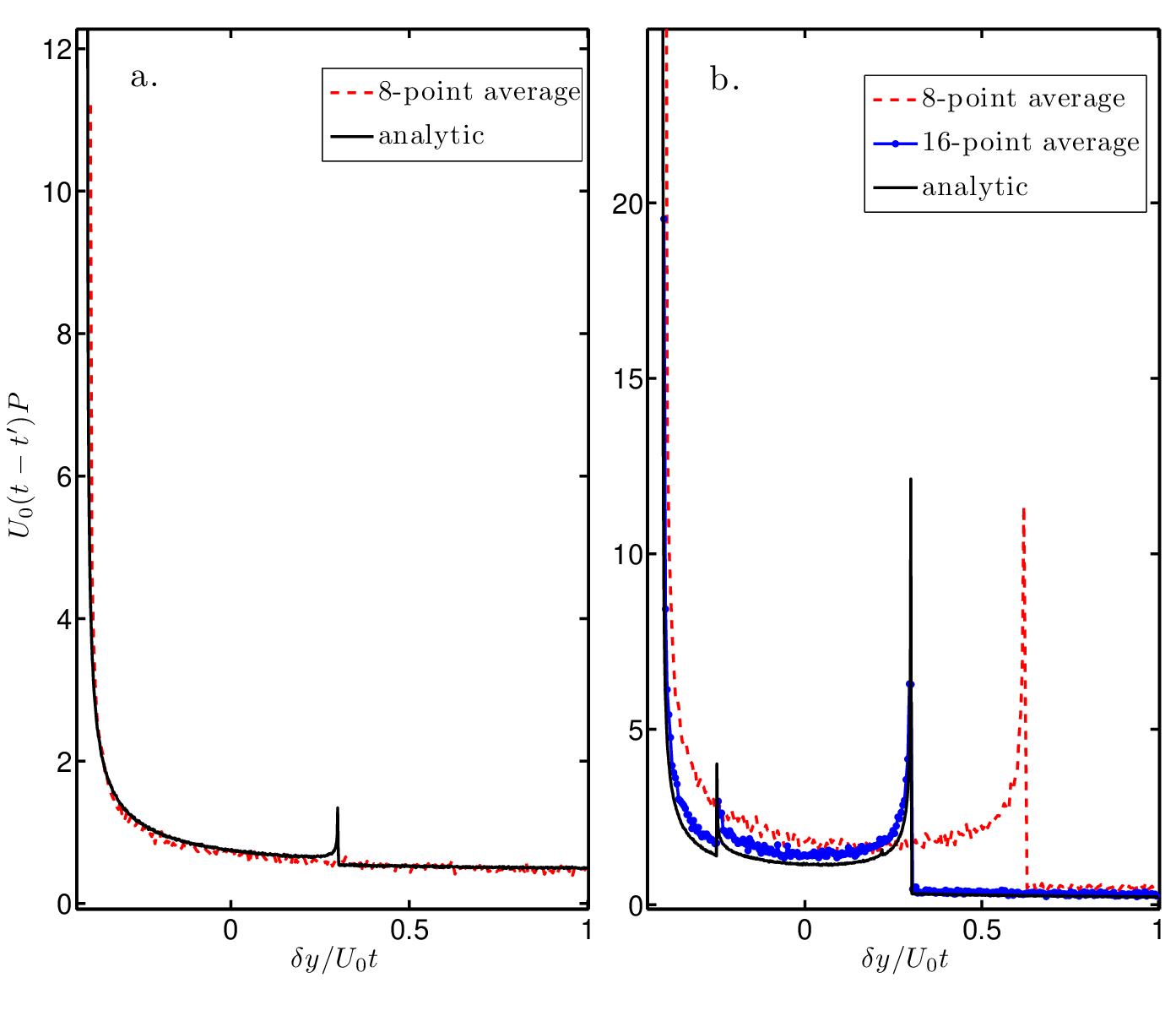
This statement is further supported by an assessment of accuracy when representing as a finite sum based on the integral
| (14) |
The Bessel function is used in spectral simulations of the gyrokinetic equation, which gives the spectral technique an advantage that we cannot use here. The Bessel integral representation may be discretized and evaluated using different numbers of terms in the sum. Additional terms in the sum reduce the error of discretization just as increasing reduces the error of discrete gyroaveraging. When the integral is approximated with or equally spaced points between and , the result agrees to with the value of up to or , respectively. For higher values of , the approximation diverges quickly, just as the discrete gyroaverage method diverges from the analytic result for increasing . Based on this, care must be taken in selecting for large values of . In this paper we restrict attention to and use an adaptive technique based on Ref. [29].
IV Diagnostics for non-diffusive transport
In this section we review several Lagrangian diagnostics for transport study. After defining each diagnostic, we recall expected behavior for both diffusive and non-diffusive transport. These diagnostics have been successfully used in transport experiments, models, and simulations in both fluids and plasmas. For examples see Refs. [27, 15, 18] and references therein. To simplify the discussion we limit attention to one-dimensional transport, i.e. transport in the poloidal-like direction . In the specific transport problem considered in this paper, is in the direction of the propagation of the zonal flow and the drift waves, and is orthogonal to both the density gradient and the magnetic field. Generalization of the diagnostics to higher dimensions is straightforward.
IV.1 Statistical moments of particle displacements
The basic particle data consists of the ensemble , with , containing the time evolution of the -coordinate of the test particles in the simulation. From here we define the ensemble of particle displacements, , where . The statistical moments of the particle displacements provide one of the simplest and most natural characterizations of Lagrangian transport. Of particular interest are the mean and the variance where denotes ensemble average. In the case of diffusive transport (e.g., a Brownian random walk), the moments exhibit asymptotic linear scaling in time, which allows the definition of an effective transport velocity (pinch) and an effective diffusivity according to and .
However, in the case of nondiffusive transport, the moments display anomalous scaling of the form
| (15) |
with and . If the spreading is slower than in the diffusive case and transport is called sub-diffusive. If , the spreading is faster than diffusion and transport is super-diffusive. A similar classification applies for sub-advection () and super-advection (). In the presence of anomalous scaling, the introduction of an effective transport velocity or an effective diffusivity is meaningless since these transport coefficients are either zero (in the sub-advection/sub-diffusion case) or infinite (in the super-advection/super-diffusion case). The diagnostics based on the statistical moments are straightforward to implement. The key is to look for a scaling region in a log-log plot of the moments as functions of time, after transients have passed. However, as with the data analyzed below, it is possible for the moments to follow different scaling regimes for different time intervals.
IV.2 Particle displacement PDFs: spatial scaling
The probability distribution function (PDF) of particle displacements, , contains all of the statistical information from displacements beyond the first and second moments. By definition, . Numerically, is constructed from the normalized histogram of particle positions at a given time. Formally, corresponds to the Green’s function determining the distribution of the test particles in terms of the initial particle distribution. For a Brownian random walk, the central limit theorem implies that asymptotically approaches a Gaussian distribution, , that satisfies diffusive scaling, , where is a Gaussian and . However, a non-diffusive propagator can exhibit the more general (anomalous) self-similar scaling
| (16) |
where and is a non-Gaussian function. Note that, by construction, the propagator has zero mean, and the scaling exponent in Eq. (16) is the same as the exponent in Eq. (15). From Eq. (16) it follows that where is a real number. Therefore, if the propagator is self-similar, is invariant with respect to the space-time renormalization transformation , up to a scale factor.
Equation (16) provides a useful diagnostic to reveal non-diffusive transport and, in particular, the existence of anomalous self- similar scaling. This diagnostic is implemented by plotting the propagator at different times in rescaled coordinates, i.e. versus . With self-similar non-diffusive transport, the plots at different times rescale and collapse into a single function . One of the most important departures from Gaussianity is algebraic decaying, “fat” tails in the propagator for large at fixed ,
| (17) |
When this behavior is found, the value of the scaling exponent is a useful diagnostic that characterizes the intermittency of the transport process.
IV.3 Trapping and flight probability distribution functions
Diffusive transport can be interpreted as a coarse-grained (macroscopic) description of a fine-grained (microscopic) Brownian random walk. In a similar way, non-diffusive transport can sometimes be viewed as the result of a non-Brownian random walk with a non-Gaussian and/or non-Markovian [30] underlying stochastic process. Trapping and flight probability distribution functions are two useful diagnostics for the characterization of non-Brownian random walks. Given a particle trajectory, , a trapping event is defined a portion of the trajectory during which the particle stays on an eddy. Flight events are portions that are not trapping events. Thus, each particle orbit in the ensemble of initial conditions may be decomposed as a sequence of trapping and flight events.
Numerically, the events are detected by tracking reversals in the Lagrangian acceleration of particles. From the histograms of trapping and flight events one may construct the probability distribution functions of trapping events, , and flight events, . Indications of non-diffusive transport can be explored by studying the departures of and from the Gaussian and exponential dependencies characteristic of Brownian random walks. Of particular interest is the presence of asymptotic algebraic scaling of the form,
| (18) |
When the mean waiting time, , is infinite and no characteristic temporal scale exists. In the Lévy flight regime , and therefore the second moment, , diverges and no characteristic spatial scale exists. The PDFs of flight and trapping events are in principle interesting because of their connection to the continuous time random walk (CTRW) model, which, in the fluid continuum limit, can be described using fractional diffusion equations [31, 32, 4].
IV.4 Lagrangian velocity autocorrelation function
Further insights into non-diffusive transport can be gained by looking at the Lagrangian velocity autocorrelation function where is the Lagrangian velocity of a particle. The Green-Kubo relation, , relates the velocity autocorrelation function to the variance of displacements. When decays fast enough so that the integral converges, this relation can be used to define an effective diffusivity according to . However, when has algebraic decay of the form
| (19) |
with , the integral diverges and the concept of effective diffusivity loses meaning. For super-diffusive transport, implies .
V Numerical results
For the Lagrangian statistics we consider ensembles of test particles, and integrate the equations of motion, with and without FLR effects, up to . The zero Larmor radius results were obtained from the numerical integration of the guiding center equations in Eq. (3) with the Hamiltonian in Eq. (9) with , , , , , . The same Hamiltonian and parameter values were used in the FLR () calculations based on an adaptive gyroaverage.
The Poincaré plots in Fig. 3 show the dependence of the degree of stochasticity on the value of . Figure 3(a) corresponds to . The degree of stochasticity is relatively large and, consistent with the results reported in Refs. [15, 1], the stochastic layer is strongly asymmetric. In particular, the region of stochasticity left of the unperturbed separatrix (shown with the bold line) is very small. As will be discussed below, this asymmetry manifests directly in the skewness of the tail of the test particle propagator, which decays strongly for due to the very low probability of having sticky-flight particles jumping in the direction. It may be interesting to compare to the thickness of the lower branch of the stochastic region, . For example, when , . This trend is mainly due to the rapid shrinkage of the stochastic layer as a function of . When , the value of is very difficult to determine because the stochastic layer has almost completely disappeared.

In the FLR calculations the test particles have a Maxwellian distribution of Larmor radii characterized by a mean value, . Thus, depending on its specific value of , each particle “sees” a different Hamiltonian, which in general will be stochastic to a lesser degree as increases. Figures 3(b)-(d) illustrate this with Poincaré plots corresponding to (b) , (c) and (d) . Each one of these Poincaré sections was computed by assigning the same value of , to all the initial conditions. It is observed that the value of has a direct non-trivial influence on the degree of stochasticity. In general, a Poincaré plot corresponding to an ensemble of particles with a Maxwellian distribution of gyroradii will be a mixture of Poincaré plots, as seen in Fig. 4. The crossings of curves in the Poincaré plots indicates the presence of multiple Hamiltonian systems indexed by values of .

To compute the Lagrangian diagnostics of non-diffusive transport, we considered groups of particles located in the vicinity of a hyperbolic equilibrium point of the Hamiltonian. The resulting trajectories can be divided into three categories: (a) passing trajectories that follow the zonal flow and never enter an eddy (vortex), (b) stagnant trajectories which never leave an eddy and (c) sticky-flight trajectories which, as shown in Fig. 5, alternate between the eddies and the zonal flow. Since the statistics of the passing and the stagnant trajectories are trivial, these particles will be ignored during the data analysis.

Several techniques for isolating sticky-flight trajectories can be devised. Our trajectory filter works by examining all trajectories during their entire history, and discarding those that never encircle a vortex (passing) and those that do not move more than one vortex width from ther original positions (stagnant). We have also tested a filter in Fourier-velocity space that discards horizontal velocity time series without a broadband spectrum. Depending on the threshold for defining “broadband,” the Fourier filter gives practically the same results as the trajectory filter. Analysis of sticky-flights in more realistic velocity fields would be served better by a Fourier-velocity filter. The proper threshold for defining a “broadband” spectrum can be found from asymptotic considerations.
Figure 6 shows the effect of the trajectory filter on the histogram of Larmor radii. In the computation of the histogram we show the number of particles, , multiplied by the appropriate metric factor . The solid line denotes the histogram considering all the particles in the ensemble, i.e. without the filter. As expected, this histogram corresponds to a sampling of the Mawellian distribution in Eq. (10). It is observed that the filter tends to remove particles with large , and, as expected, the number of particles removed decreases with , the time of filter application. Since appears to give an asymptotic value for the number of sticky-flights, it is used as the filtering time for the following diagnostics. When scaling values are reported for , the filter is still applied uniformly at . The first column in Table 1 gives , the percentage of sticky-flights, for each tested value of when the filter is applied at .

| 0.0 | 96 | 1.1 | 1.0 | 1.9 | 1.6 | 2.0 |
|---|---|---|---|---|---|---|
| 0.001 | 96 | 1.1 | 1.0 | 1.9 | 1.6 | 2.0 |
| 0.01 | 96 | 1.1 | 1.0 | 1.9 | 1.6 | 2.0 |
| 0.1 | 98 | 1.1 | 1.1 | 2.0 | 1.8 | 2.2 |
| 0.2 | 97 | 1.1 | 1.1 | 2.0 | 1.8 | 2.3 |
| 0.4 | 96 | 1.1 | 1.1 | 1.9 | 1.9 | 2.3 |
| 0.6 | 92 | 1.1 | 1.0 | 1.9 | 1.9 | 2.7 |
| 0.8 | 83 | 1.1 | 1.1 | 1.9 | 1.9 | 2.7 |
| 1.2 | 58 | 0.9 | 1.0 | 1.8 | 1.8 | 2.9 |
| 1.6 | 36 | 0.8 | 1.0 | 1.8 | 1.8 | 2.9 |
| 3.0 | 11 | 0.9 | 0.9 | 1.8 | 1.6 | 3.1 |
V.1 Super-diffusive scaling
Before presenting the chaotic transport results, it is instructive to go back to the simple parallel flow in Eq. 11 to explore the role of FLR effects on particle dispersion in the context of an integrable flow for a ensemble of particles initially distributed according to . If all the particles have the same Larmor radius, i.e. if , then as Eq. 29 in Appendix A shows, maintains its delta function shape and simply drifts with the effective velocity , which in the limit of zero Larmor radius corresponds to the parallel flow velocity. In this case, FLR effects are irrelevant since they simply rescale the velocity. However, when the particles have different Larmor radii, as in the Maxwellian case of Eq. 30, the effective velocity of each particle will be different and the initial delta function will spread in space as is evident in the particle propagators shown in Fig. 2. In this case, the first and second moments are and , where and A are functions of given in Appendix A. The key issue to observe is that the variance does not exhibit diffusive scaling, and that a distribution of Larmor radii gives rise to a ballistic spreading of the particles.
For transport in the nonintegrable flow with the zonal flow and drift waves, Fig. 7 shows the mean, , and variance, , for and . A summary of the values of the scaling exponents and for all the values of studied is presented in Table 1. To a good approximation, the mean exhibits linear scaling, i.e. in Eq. (15), indicative of regular advection, for all values of . The variance consistently shows clear evidence of super-diffusive transport, i.e. in Eq. (15). In the zero Larmor radius case, two scaling regimes are observed. Up to , which corresponds to the simulations in Ref. [15], the power law fitting in Fig. 7(b) indicates an almost ballistic scaling with . However, at a later time there is a transition to . As Table 1 shows, FLR effects seem to eliminate the distinction between early and late regimes. In particular, according to Fig. 7(d) where , the scaling holds throughout the integration time. As a general trend, it is observed that the exponent decreases with increasing beyond . Statistics for sticky-flights become poor for because the degree of stochasticity [see Fig. 3(d)] becomes small.

V.2 Asymmetric, non-Gaussian PDF of particle displacements
Motivated by the presence of two different scaling regimens in the variance, we study the PDF of particle displacements at intermediate and large times. Figure 8 shows the PDFs at intermediate times, with 8(a) corresponding to and 8(b) corresponding to . The solid lines denote the PDFs of the filtered data, (i.e. including only sticky-flight orbits) and the dashed line denotes the PDFs of the unfiltered data. The spikes for large in the unfiltered distributions result from the contribution of passing orbits that the filter effectively removes. The filtered PDFs are clearly non-Gaussian with strong skewness in the negative direction. The strong left-right asymmetry of the PDFs results from the asymmetry of the stochastic layer.

In particular, as the Poincaré plots in Fig. 3 show, the stochastic layer is thicker on the right side of the vortex. This asymmetry depends on the value of the perturbation frequency in Eq. (9). In fact, as discussed in Ref. [15], the relative thickness of the stochastic layers, and therefore the symmetry of tracer transport, can be controlled by changing . As the insets in Fig. 7 show, both PDFs decay algebraically as in Eq. (17). However, a strong dependence of the decay exponent on the value of the Larmor radius is observed. For , , and for , . As Table 1 indicates, the value of the decay exponent increases monotonically with .
The particle displacement PDFs at longer times are shown in Fig. 9. As before, the solid lines denote the filtered distribution and the dashed lines the unfiltered distribution. A critical dependence on the Larmor radius is observed. For the PDF transitions to an exponential decaying distribution, whereas for the PDF maintains its algebraic decay with the same exponent as the one observed at short times, . The robustness of the algebraic decay in the finite Larmor radius case might be attributed to the persistence of large particle displacements which, due to the presence of the strong zonal flows, are enhanced by the gyroaverage. One should note that a Lévy process requires , which means that the increase of moves the process away from the Lévy type.

The transition from algebraic to exponential decay in the zero Larmor radius case is likely due to the presence of truncated Lévy flights. Exact Lévy flights produce long particle displacements that result in slowly decaying algebraic tails at all times. However, non-ideal effects such as particle decorrelation might preclude the existence of arbitrarily long displacements, resulting in a faster than algebraic decay of the tails at long times. See, for example, Refs. [33, 34, 35] for more details on truncated Lévy processes. One obvious reason for a truncated Lévy process in the present system is the finite velocity requirement, which precludes the existence of infinite jumps.
V.3 Lévy flights and algebraic trapping PDFs
Figure 10 shows the trapping time and flight length PDFs for in (a) and (c), and for in (b) and (d). In both cases, the trapping PDF clearly decays algebraically as in Eq. (18), with for , and for . Figures 10(c) and 10(d) show the PDFs of flight lengths. Note that, because transport in this case is asymmetric, there are actually two flight PDFs, one corresponding to positive flights (with dashed fit line) and another corresponding to negative flights (solid fit line). The PDF of negative flights decays as a power law with for , and for . Since in both cases, these flights correspond to Lévy flights. However, the decay of the curve for positive flights is much steeper with regardless of the value of , which implies that positive displacements are not Lévy flights. The tails of the trapping and flight PDFs transition to exponential decay at and . As discussed before, this transition is indicative of the possible presence of truncated Lévy flights.

V.4 Algebraic decay of Lagrangian velocity autocorrelation function
Figure 11 shows the Lagrangian velocity autocorrelation function for the sticky-flights with in Fig. 11(a) and with in Fig. 11(b). Both curves follow algebraic decay of the form . When , and when , . Both values are consistent with the Green-Kubo relation between the decay of the velocity correlation and the scaling of the variance according to which . The frequency of small scale oscillations observed in the correlation seems to increase when changes from .

VI Self-similar anomalous scaling and fractional diffusion modeling
An important goal of transport modeling is to construct effective transport equations that describe the “macroscopic” coarse grained dynamics when given information at the “microscopic” kinetic level. When the microscopic dynamics involves Gaussian, Markovian stochastic processes (e.g., a Brownian random walk) the macroscopic dynamics can be modeled using diffusion type equations. This is the basic idea behind the use of diffusive models to describe collisional transport. However, in recent years it has been shown that the standard diffusion picture can fail when non- Gaussian and/or non-Markovian statistics are present.
In particular, experimental, numerical and analytical transport studies in fluids and plasmas (e.g. Refs. [11, 36, 37, 38, 15, 16, 18, 39, 40, 25] and references therein) have shown that underlying stochastic processes governing particle transport in flows with coherent structures, like zonal flows and eddies, typically involve anomalously large particle displacements induced by the zonal flows and/or anomalous particle trapping in eddies. The presence of large particle displacements can invalidate the Gaussianity of displacement distributions. Particle trapping can introduce waiting time effects that invalidate the Markovian assumption because of memory effects. The statistics of particle transport discussed in the previous section shows clear evidence of these type of phenomena. This section presents an effective macroscopic model that describes quantitatively the spatio-temporal evolution of the PDF of particle displacements.
An important piece of information needed for constructing an effective transport model is shown in Fig. 12. Figures 12(a)-(c) show the temporal evolution of the PDF of particle displacements for different values of . As discussed before, the PDF develops a strong “fat” tail to the left and, by conservation of probability, the peak of the distribution goes down. Figures 12(d)-(f) show the same data plotted using rescaled variables as in Eq. (16). In the horizontal axis, , and in the vertical axis, has been multiplied by the factor , where is the anomalous diffusion exponent in Eq. (15). From this it follows that the PDF at a time is related to the PDF at time by the scaling transformation . The fact that, for the problem of interest here, , rules out the possibility of constructing a transport model based on the diffusion equation with an effective diffusivity because the solution of the diffusion equation scales as .

A natural way to built transport models that display self-similar anomalous scaling is to use fractional diffusion equations of the from
| (20) |
where , and . The operators and are called the left and right fractional derivatives. These non-local operators are a natural generalization of the regular differential operator, , of integer order . For example, Fourier transforms of the fractional operator, , satisfy
| (21) |
for non-integer values of . In a similar way, the operator on the left hand side of Eq. (20) is a natural extension of the regular time derivative, , in the sense that its Laplace transform, , satisfies
| (22) |
for . As expected, Eq. (20) reduces to the standard diffusion equation when and . Further formal details on fractional derivatives, including their representation in the and domains in terms of non-local operators can be found in Refs. [41, 42]. For a discussion on the use of these operators to model non-diffusive transport in plasmas, see for example Refs. [18, 19] and references therein.
To explore the self-similarity properties of the fractional diffusion model we use Eqs. (21)-(22) and write the Fourier-Laplace transform, , of the Green’s function, , of Eq. (20) as
| (23) |
where and . It follows directly from Eq. (23) that which in - space implies the self-similar scaling of the fractional diffusion propagator Eq. (20). Therefore, the fractional equation will exhibit the same self-similar scaling as the numerically obtained PDF provided the fractional orders of the spatial and temporal derivatives satisfy
| (24) |
According to Table 1, to a good approximation, in the intermediate asymptotic regime. Based on this observation, and following Eq. (24), we will assume in the fractional diffusion model. This special case, known as neutral fractional diffusion, has a Green’s function that can fortunately be expressed in closed form using elementary functions, as shown in Ref. [43]:
| (25) |
where is the similarity variable and . The solution for is obtained using the relation . The parameter is related to the asymmetry parameter introduced before in the definition of the weighting factors and according to . Given the Green’s function, the solution of the fractional diffusion equation for an initial condition is
| (26) |

For the initial condition we assume a localized distribution of the form for and elsewhere (see Ref. [18]). The use of this initial condition is necessary to account for the presence of transients in the evolution of the PDF not reproduced by the fractional diffusion equation, which describes the intermediate time regime. Figure 13 shows the comparison of the solution of the fractional diffusion equation in Eq. (20) according to Eqs. (26) and (25) and the numerically obtained PDF obtained from the histograms of particle displacements at for in Fig. 13(a) and in Fig. 13(b). For the fractional diffusion model parameters we used and in the case, and and in the case. In both cases, we used , which is small compared to the maximum range of the PDF, .
VII Summary and conclusions
In this paper we presented a numerical study of FLR effects on non-diffusive transport of test particles in a flow dominated by a strong zonal shear flow and large scale eddies. We modeled the flow using a Hamiltonian dynamical system consisting of a linear superposition of a strong zonal shear flow and eigenmodes of the HM equation. For the parameter values considered, the Hamiltonian causes chaotic transport. Test particles alternate stochastically between being trapped in the vortices and being transported by the zonal flow. To expose the non-diffusive properties of the system we used Lagrangian statistical diagnostics including: (i) the scaling in time of statistical moments; (ii) the PDFs of particle displacements, (iii) trapping events and (iv) flight events; and (v) the decay of the Lagrangian velocity autocorrelation function.
Finite Larmor radius effects were incorporated in the particle calculations by substituting the value of the velocity at the location of the guiding center by its value averaged over a ring of radius , where is the Larmor radius. The ring average was computed using a discrete approximation. The numerical method was benchmarked using an analytical solution for a parallel zonal flow with no waves. We found that for an -point average gives accurate results, but higher order approximations must be used for for . Contrary to previous works where all the particles were assumed to have the same value of , here we considered a more realistic Maxwellian distribution of Larmor radii. Poincaré plots revealed that the Larmor radius has a direct nontrivial effect on the topology of the flow and the degree of chaos of test particles. In particular, it was observed that the amount of chaos, measured by the width of the stochastic region, is significantly reduced as increases from to . A distribution of Larmor radii can also have a direct effect on the dispersion of particles. In particular, we have shown that, even in the case of a completely integrable flow, particles exhibit ballistic spreading, , when they have different Larmor radii.
For the Lagrangian statistics we limited attention to sticky-flight orbits and ignored trapped and passing orbits. The rationale for this filter is that the trivial dynamics of passing and trapped particles give rise to outliers that artificially bias the statistics. The first moment, to a good approximation, has normal advective scaling, i.e. , with , and the second moment has super-diffusive scaling, i.e. , with . For , a sharp transition was observed in the scaling exponent, from at intermediate times to at larger times. Similar transitions in the value of have been also found in other systems including temporally irregular channel flows [36], time dependent, three dimensional flows [44], and two-dimensional vortex flows [16]. For specific experimental instances, early time behavior will be more important than late time behavior if the domain crossing time is small enough. We have found that FLR effects seem to eliminate the distinction between early and late time. For the range of considered, . We refer to this regime as super-diffusive ballistic transport since the variance approaches ballistic scaling () but the PDF of displacements retains a super- diffusive appearance. Complementary results were obtained in Ref. [12] for nonlinear HM simulations.
We also observed that the Lagrangian velocity autocorrelation function decays algebraically, where, in reasonable agreement with the Green-Kubo scaling, . The trapping and flight distributions show algebraic decay. The trapping time exponent, , remains the same when changes. The PDFs of negative flights qualify as truncated Lévy distributions but positive flights are definitively not Lévy. The negative flight exponent for is larger than expected in the context of a CTRW.
At intermediate times, consistent with Refs. [15, 1], the PDF of particle displacements in the zero Larmor radius case is an asymmetric non-Gaussian distribution with an algebraic decaying leftward tail. However, for larger times, the tail of the PDF transitions from algebraic to exponential decay. This algebraic-exponential transition in the PDF is likely to be related to the presence of truncated Lévy flights, which, as discussed in Ref. [35], might result from particle decorrelation or the finite size of possible displacements. The robustness of the algebraic decay in the finite Larmor radius case might be attributed to the persistence of large particle displacements which, due to the presence of the strong zonal flows, are enhanced by the gyroaverage. We have also shown that the PDF of particle displacements has self-similar scaling behavior for and . Most importantly, we have shown that these distributions correspond to solutions of the neutral () asymmetric fractional diffusion equation.
Future work will apply the ideas and tools developed here to turbulent flows to more realistic plasma turbulence models. In particular, we will examine self-consistent particle transport parallel to a density gradient in a gyrokinetic particle-in-cell simulation. Transport properties of tracers and self-consistent particles should be compared.
Acknowledgements.
Thanks to T.M. Antonsen, Jr., S. Brunner, P. Ricci, M. Barnes and I. Broemstrup for helpful discussions. This work is supported by the Fannie and John Hertz Foundation. Additional support comes from the Oak Ridge National Laboratory, managed by UT-Battelle, LLC, for the U.S. Department of Energy under Contract DE-AC05-00OR22725 and from the DOE Center for Multiscale Plasma Dynamics, Grant DE- FC02-04ER54784.Appendix A Gyro-averaged particle propagator in a parallel flow
The gyroaverage equations of motion for test particles in the parallel zonal flow of Eq. 11 are
| (27) |
A straightforward integration assuming an intial condition gives
| (28) |
where . From here it follows that the two-dimensional propagator is
| (29) |
Integrating over and assuming a Maxwellian distribution of gyroradii gives the one-dimensional propagator in ,
| (30) |
Integrating over using basic properties of the delta function gives Eq. 12. From Eq. (30) it follows that the -th moment of the gyrocenter displacement scales like according to
| (31) |
where is the gyroradii distribution function. For and we recover the moments in Sec. V(A) with
| (32) |
in the case when is Maxwellian, where is the modified Bessel function of zero-order. It is interesting to note that has a maximum for .
References
- [1] D. del Castillo Negrete, Phys. Plasmas 7, 1702 (2000).
- [2] A. Hasegawa and K. Mima, Physics of Fluids 21, 87 (1978).
- [3] W. W. Lee, Journal of Computational Physics 72, 243 (1987).
- [4] R. Metzler and J. Klafter, Physics Reports 339, 1 (2000).
- [5] J.-P. Bouchaud and A. Georges, Physics Reports 195, 127 (1990).
- [6] R. Balescu, Aspects of Anomalous Transport in Plasmas (IOP Puslishing, Bristol, 2005).
- [7] D. del Castillo-Negrete, in Turbulent transport in fusion plasmas: First ITER International Summer School, edited by S. Benkadda (AIP, College Park, 2008).
- [8] W. Horton, Plasma Physics 23, 1107 (1981).
- [9] G. Manfredi and R. Dendy, Phys. Rev. Lett. 76, 4360 (1996).
- [10] G. Manfredi and R. Dendy, Phys. Plasmas 4, 628 (1997).
- [11] S. Benkadda, P. Gabbai, and G. M. Zaslavsky, Phys. Plasmas 4, 2864 (1997).
- [12] S. Annibaldi, G. Manfredi, R. Dendy, and L. Drury, Plasma Phys. Control. Fusion 42, L13 (2000).
- [13] S. V. Annibaldi, G. Manfredi, and R. O. Dendy, Phys. Plasmas 9, 791 (2002).
- [14] W. Horton and A. Hasegawa, Chaos 4, 227 (1994).
- [15] D. del Castillo Negrete, Phys. Fluids 10, 576 (1998).
- [16] S. Kovalyov, Chaos 10, 153 (2000).
- [17] A. Chechkin, V. Gonchar, and M. Szydlowski, Phys. Plasmas 9, 78 (2002).
- [18] D. del Castillo Negrete, Phys. Plasmas 11, 3854 (2004).
- [19] D. del Castillo Negrete, Phys. Plasmas 13, 082308 (2006).
- [20] L. Garcia and B. A. Carreras, Physics of Plasmas 13, 022310 (2006).
- [21] D. del Castillo-Negrete et al., Nuclear Fusion 48, 075009 (13pp) (2008).
- [22] I. Calvo et al., Physics of Plasmas 15, 042302 (2008).
- [23] F. Jenko and W. Dorland, Phys. Rev. Lett. 89, 225001 (2002).
- [24] I. Furno et al., Physical Review Letters 100, 055004 (2008).
- [25] T. Hauff, F. Jenko, and S. Eule, Physics of Plasmas 14, 102316 (2007).
- [26] H. Aref, Journal of Fluid Mechanics 143, 1 (1984).
- [27] T. Solomon, E. R. Weeks, and H. L. Swinney, Physical Review Letters 71, 3975 (1993).
- [28] J. M. Finn and D. del Castillo Negrete, Chaos 11, 816 (2001).
- [29] A. Mishchenko, A. Könies, and R. Hatzky, Phys. Plasmas 12, 062305 (2005).
- [30] M. Shlesinger, G. M. Zaslavsky, and J. Klafter, Nature (London) 31, 363 (1993).
- [31] E. W. Montroll and G. H. Weiss, Journal of Mathematical Physics 6, 167 (1965).
- [32] E. W. Montroll and M. F. Shlesinger, in Nonequilibrium Phenomena II. From Stochastics to Hydrodynamics, edited by J. L. Lebowitz and E. W. Montroll (Elsevier, Amsterdam, 1984).
- [33] R. N. Mantegna and H. E. Stanley, Physical Review Letters 73, 2946 (1994).
- [34] I. Koponen, Phys. Rev. E 52, 1197 (1995).
- [35] A. Cartea and D. del Castillo-Negrete, Physical Review E 76, 041105 (2007).
- [36] S. C. Venkataramani, T. M. Antonsen, Jr., and E. Ott, Physical Review Letters 78, 3864 (1997).
- [37] E. R. Weeks and H. L. Swinney, Phys. Rev. E 57, 4915 (1998).
- [38] F. Dupont, R. I. McLachlan, and V. Zeitlin, Phys. Fluids 10, 3185 (1998).
- [39] T. Benzekri et al., Phys. Rev. Lett. 96, 124503 (2006).
- [40] S. V. Prants, M. V. Budyansky, and M. Y. Uleysky, Chaos 16, 033117 (2006).
- [41] I. Podlubny, Fractional Differential Equations (Academic Press, San Diego, 1999).
- [42] S. G. Samko, A. A. Kilbas, and O. I. Marichev, Fractional Integrals and Derivatives: Theory and Applications (Taylor and Francis Books Ltd, London, 1993).
- [43] F. Mainardi, Y. Luchko, and G. Pagnini, Fract. Calc. App. Analysis 4, 153 (2001).
- [44] M. A. Fogleman, M. J. Fawcett, and T. H. Solomon, Physical Review E 63, 020101 (2001).