Information filtering based on transferring similarity
Abstract
In this Brief Report, we propose a new index of user similarity, namely the transferring similarity, which involves all high-order similarities between users. Accordingly, we design a modified collaborative filtering algorithm, which provides remarkably higher accurate predictions than the standard collaborative filtering. More interestingly, we find that the algorithmic performance will approach its optimal value when the parameter, contained in the definition of transferring similarity, gets close to its critical value, before which the series expansion of transferring similarity is convergent and after which it is divergent. Our study is complementary to the one reported in [E. A. Leicht, P. Holme, and M. E. J. Newman, Phys. Rev. E 73 026120 (2006)], and is relevant to the missing link prediction problem.
pacs
89.75.Hc, 87.23.Ge, 05.70.LnWith the exponential growth of the Internet [1] and the World-Wide-Web [2], a prominent challenge for modern society is the information overload. Since there are enormous data and sources, people never have time and vigor to find out those most relevant for them. A landmark for solving this problem is the use of search engine [3, 4]. However, a search engine could only find the relevant web pages according to the input keywords without taking into account the personalization, and thus returns the same results regardless of users’ habits and tastes. Thus far, with the help of Web2.0 techniques, personalized recommendations become the most promising way to efficiently filter out the information overload [5]. Motivated by the significance in economy and society, devising efficient and accurate recommendation algorithms becomes a joint focus from theoretical studies [5] to e-commerce applications [6]. Various kinds of algorithms have been proposed, such as collaborative filtering (CF) [7, 8], content-based methods [9, 10], spectral analysis [11, 12, 13], principle component analysis [14], network-based inference [15, 16, 17, 18], and so on.
A recommender system consists of users and objects, and each user has rated some objects. Denoting the user set as and the object set as , the system can be fully described by an rating matrix V, with denoting the rating user gives to object . If has not yet evaluated , is set as zero. CF system has been one of the most successfully and widest used recommender systems since its appearance in the mid-1990s [7, 8]. Its basic idea is that the user will be recommended objects based on the weighted combination of similar users’ opinions. In the standard CF, the predicted rating from user to object is set as:
| (1) |
where is the similarity between and , means the average rating of and serves as the normalization factor. Here, runs over all users having rated object excluding himself. The similarity, , plays a crucial role in determining the algorithmic accuracy. In the implementation, the similarity between every pair of users is calculated firstly, and then the predict ratings by Eq. (1). Various similarity measures has been proposed, among which the Pearson correlation coefficient is the widest used [7], as:
| (2) |
where , and run over all the objects commonly selected by user and . All diagonal elements in the similarity matrix are set to be zero.
Several algorithms [19, 20, 21] have recently been proposed to improve the accuracy of the standard CF via modifying the definition of user-user similarity. However, all those algorithms have not fully addressed the similarity induced by indirect relationship, say, the high-order correlations. Note that, the Pearson correlation coefficient, , considers only the direct correlation. We argue that to appropriately measure the similarities between users, the indirect correlations should also be taken into consideration. To make our idea clearer, we draw an illustration in Fig. 1. Suppose there are three users, labeled as , and . Although the similarity between user and is quite small, and are both very similar with . Actually, , and may share very similar tastes, and the very small similarity between and may be caused by the sparsity of the data. That is to say, and has a very few commonly selected objects. The sparsity of data set makes the direct similarity less accurate, and thus we expect a new measure of similarity properly integrating high-order correlations may perform better.


Denoting a decay factor of similarity transferred by a medi-user, a self-consistent definition of transferring similarity can be written as:
| (3) |
where is the direct similarity as shown in Eq. (2). The parameter can be considered as the rate of information aging by transferring one step further [22]. Clearly, the transferring similarity will degenerate to the traditional Pearson correlation coefficient when . Denoting and the direct similarity matrix and the transferring similarity matrix, Eq. (3) can be rewritten in a matrix form, as:
| (4) |
whose solution is
| (5) |
Accordingly, the prediction score reads
| (6) |
where multiplier serves as the normalizing factor and runs over all users having rated object excluding himself.
| Data Divisions | 90% vs. 10% | 50% vs. 50% | 10% vs. 90% |
|---|---|---|---|
| 0.0061 | 0.0063 | 0.0156 | |
| 0.006136 | 0.006311 | 0.015642 |
To test the algorithmic accuracy, we use a benchmark data set, namely MovieLens, which consists of users, objects, and discrete ratings from 1 to 5. The sparsity of the rating matrix V is about 6%. We first randomly divide this data set into two parts: one is the training set, treated as known information, and the other is the probe, whose information is not allowed to be used for prediction. Then we make a prediction for every entry contained in the probe (resetting and in the case of and , respectively), and measure the difference between the predicted rating and the actual rating . For evaluating the accuracy of recommendations, many different metrics have been proposed [7]. We choose two commonly used measures: root-mean-square error (RMSE) and mean absolute error (MAE). They are defined as
| (7a) | ||||
| (7b) | ||||
where the subscript runs over all the elements in the probe, and is the number of those elements.
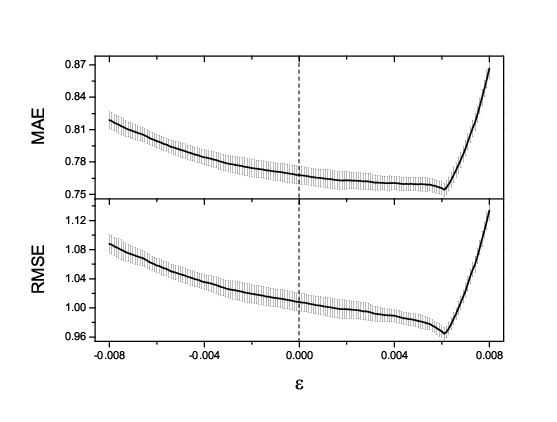
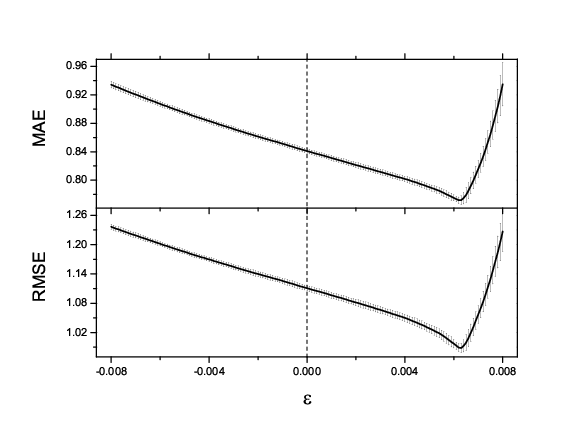
In Figs. 2-4, we report the numerical results about the algorithmic accuracy, where the divisions of training set and probe are 90% vs. 10%, 50% vs. 50%, and 10% vs. 90%, respectively. In every case, there exists an optimal value of , denoted by , corresponding to both the lowest MAE and the lowest RMSE. Around the optimal value, , the present algorithm obviously outperforms the standard CF. The optimal values are different for different cases, and the one corresponding to sparser data is larger.
To get some insights about the physical meaning of , we expand Eq. (5) by a power series, as:
| (8) |
Note that, this formula is also of practical significance since to directly inverse takes long time for huge-size systems, and the cutoff of Eq. (8),
| (9) |
is usually used as an approximation in the implementation (in this paper, since the system size in not too large, we always directly use Eq. (5) to obtain the transferring similarity matrix). However, even if is inversable, Eq. (8) may not be convergent. Actually, Eq. (8) is convergent if and only if all the eigenvalues of are strictly smaller than 1. The mathematical proof of a very similar proposition using Jordan matrix decomposition can be found in Ref. [22]. Although Ref. [22] only gives the proof of the sufficient condition, the necessary condition can be proved in an analogical way. Accordingly, there exists a critical point of , before which the spectral radius of is less than 1 and after which it exceeds 1. Since this critical value is also the maximal value of that keeps the convergence of Eq. (8), we denote it by . The optimal and maximal values of for the three cases corresponding to Figs. 2-4 is presented in Table 1. It is very interesting that is always smaller yet very close to .
In summary, we designed an improved collaborative filtering algorithm based on a newly proposed similarity measure, namely the transferring similarity. Different from the traditional definitions of similarity that consider the direct correlation only, the transferring similarity integrates all the high-order (i.e., indirect) correlations. The numerical testing on a benchmark data set has demonstrated the improvement of algorithmic accuracy compared with the standard CF algorithm. Very recently, Zhou et al. [23] and Liu et al. [21] proposed some modified recommendation algorithms under the frameworks of collaborative filtering [21] and random-walk-based recommendations [23],respectively. By taking into account both the direct and the second order correlations, their algorithms can remarkably enhance the prediction accuracy. These work can be considered as a bridge connecting the nearest-neighborhood-based information filtering algorithms and the present work.
Very interestingly, we found that the optimal value of is always smaller yet very close to the maximal value of that guarantees the convergence of power series expansion of the transferring similarity. The significance of this finding is twofold. Firstly, Leicht, Holme and Newman [24] have recently proposed a new index of node similarity, which is actually a variant of the well-known Katz index [25]. The numerical tests [24] showed that their index best reproduces the known correlations between nodes when the parameter is very close to its maximal value that guarantees the convergence of power series expansion. Although their work and the current work originate from different motivations and use different testing methods, the results are surprisingly coincident. Despite the insufficiency of empirical studies and the lack of analytical insights, this finding should be of theoretical interests. Secondly, is equal to the inverse of the maximum eigenvalue of S, . Therefore, it is easy to determine since fast algorithms on calculating for a given matrix is well developed (see, for example, the power iteration method in Ref. [26]). When dealing with an unknown system, we can first calculate , and then concentrate the search of on the area around , which can save computations in real applications.
Very recently, a fresh issue is raised to physics community, that is, how to predict missing links of complex networks [27, 28]. The fundamental problem is to determine the proximities, or say similarities, between node pairs [29, 30]. The similarity index presented here is not only an extension of the Pearson correlation coefficient in rating systems, but also easy to be extended to quantify the structural similarity of node pair in general networks based on any locally defined similarity indices. We believe this self-consistent definition of similarity (see Eq. (3)) can successfully find its applications in link prediction problem.
We acknowledge GroupLens Research Group for MovieLens data (http://www.grouplens.org). This work is supported by the 973 Project 2006CB705500, and the National Natural Science Foundation of China under Grant Nos. 60744003 and 10635040. T.Z. and J.-G.L. acknowledge the support from SBF (Switzerland) for financial support through project C05.0148 (Physics of Risk), and the Swiss National Science Foundation (205120-113842).
References
- [1] G.-Q. Zhang, G.-Q. Zhang, Q.-F. Yang, S.-Q. Cheng, and T. Zhou, New J. Phys. 10, 123027 (2008).
- [2] A. Broder, R. Kumar, F. Moghoul, P. Raghavan, S. Rajagopalan, R. Stata, A. Tomkins, J. Wiener, Comput. Netw. 33, 309 (2000).
- [3] S. Brin, L. Page, Computer Networks and ISDN Systems 30, 107 (1998).
- [4] J. M. Kleinberg, J. ACM 46, 604 (1999).
- [5] G. Adomavicius, and A. Tuzhilin, IEEE Trans. Know. Data Eng. 17, 734 (2005).
- [6] J. B. Schafer, J. A. Konstan, and J. Riedl, Data Mining and Knowledge Discovery 5, 115 (2001).
- [7] J. L. Herlocker, J. A. Konstan, K. Terveen, and J. T. Riedl, ACM Trans. Inform. Syst. 22, 5 (2004).
- [8] J. A. Konstan, B. N. Miller, D. Maltz, J. L. Herlocker, L. R. Gordon, and J. Riedl, Commun. ACM 40, 77 (1997).
- [9] M. Balabanović, and Y. Shoham, Commun. ACM 40, 66 (1997).
- [10] M. J. Pazzani, Artif. Intell. Rev. 13, 393 (1999).
- [11] D. Billsus, and M. Pazzani, Proc. Int’l Conf. Machine Learning (1998).
- [12] B. Sarwar, G. Karypis, J. A. Konstan, and J. T. Riedl, Proc. ACM WebKDD Workshop (2000).
- [13] J. Ren, T. Zhou, and Y.-C. Zhang, Europhys. Lett. 82, 58007 (2008).
- [14] K. Goldberg, T. Roeder, D. Gupta, and C. Perkins, Inform. Ret. 4, 133 (2001).
- [15] Y.-C. Zhang, M. Blattner, and Y.-K. Yu, Phys. Rev. Lett. 99, 154301 (2007).
- [16] Y.-C. Zhang, M. Medo, J. Ren, T. Zhou, T. Li, and F. Yang, Europhys. Lett. 80, 68003 (2007).
- [17] T. Zhou, J. Ren, M. Medo, and Y.-C. Zhang, Phys. Rev. E 76, 046115 (2007).
- [18] T. Zhou, L. L. Jiang, R. Q. Su, Y.-C. Zhang, Europhys. Lett. 81, 58004 (2008)
- [19] J.-G. Liu, B.-H. Wang, and Q. Guo, Int. J. Mod. Phys. C (to be published).
- [20] R.-R. Liu, C.-X. Jia, T. Zhou, D. Sun, and B.-H Wang, Physica A 388, 462 (2009).
- [21] J.-G. Liu, T. Zhou, B.-H. Wang, and Y.-C. Zhang, arXiv: 0808.3726.
- [22] A. Stojmirovic and Y.-K. Yu, J. Comput. Biol. 14, 1115 (2007).
- [23] T. Zhou, R.-Q. Su, R.-R. Liu, L.-L. Jiang, B.-H. Wang, and Y.-C. Zhang, arXiv: 0805.4127.
- [24] E. A. Leicht, P. Holme, and M. E. J. Newman, Phys. Rev. E 73, 026120 (2006).
- [25] L. Katz, Psychmetrika 18, 39 (1953).
- [26] G. H. Golub and C. F. Von Load, Matrix Computation (Johns Hopkins University Press, Baltimore, 1996).
- [27] A. Clauset, C.Moore, M. E. J. Newman, Nature 453, 98 (2008).
- [28] S. Redner, Nature 453, 47 (2008).
- [29] D. Liben-Nowell and J. Kleinberg, J. Am. Soc. Inform. Sci. Technol. 58, 1019 (2007).
- [30] T. Zhou, L. Lü, and Y.-C. Zhang, arXiv: 0901.0553.