Shear Viscosity of the Outer Crust of Neutron Stars: Ion Contribution
Abstract
The shear viscosity of the crust might have a damping effect on the amplitude of r-modes of rotating neutron stars. This damping has implications for the emission of gravitational waves. We calculate the contribution to the shear viscosity coming from the ions using both semi-analytical methods, that consider binary collisions, and Molecular Dynamics simulations. We compare these results with the contribution coming from electrons. We study how the shear viscosity depends on density for conditions of interest in neutron star envelopes and outer crusts. In the low density limit, we find good agreement between results of our molecular dynamics simulations and classical semi-analytic calculations.
pacs
97.60.Jd, 26.60.Gj, 52.25.Fi, 26.50.+xI Introduction
Neutron stars are good resonators where oscillation modes can be excited. In particular, the r-modes of rotating neutron stars involve currents associated with very small density variations. These modes are unstable at all rates of rotation in a perfect fluid star [1]. The instability is due to the emission of gravitational radiation, suggesting the possibility of gravitational wave detection with Laser Interferometer Gravitational-Wave Observatory (LIGO) [2]. This instability is expected to spin down newly born hot neutron stars [3]. However, the observation of colder rapidly rotating neutron stars, suggests the existence of a damping mechanism of the r-mode instability. Several works have been done to explain this mechanism. For example, in Ref. [4] the damping mechanism is suggested to be the result of a viscous layer at the interface between the solid crust and the fluid core. Other works discuss the r-mode dynamics of superfluid neutron stars [5, 6] finding that a core filled with neutron and proton superfluids limits the amplitude growth of the modes [7]. In addition, high multipolarity p-mode oscillations may impact the pulse shape of some radio pulsars [8]. For p-modes the primary restoring force is the pressure and the modes may be damped by the shear viscosity of the neutron star crust [9].
In the outer crust, the total shear viscosity has contributions from electrons and ions both of which transport momentum. Previous works have calculated the electron contribution to the shear viscosity in the Born approximation [10] and including non-Born corrections [9]. Recently Horowitz and Berry calculated the electron contribution to the shear viscosity of non-spherical nuclear pasta phases [11]. In this work we study the dependency of the shear viscosity with the density. We calculate the contribution of the ions to the shear viscosity in the neutron stars crust by two different methods: via Molecular Dynamics (MD) simulations and calculating momentum transport cross sections. The first method follows the Kubo formalism [12], and calculates the autocorrelation function of the pressure tensor. The second method considers binary collisions and allows one to consider both the classical and quantum systems. We focus our study to the case in which the ions form a dilute Hydrogen One Component Plasma (OCP). The conditions of temperature and density are chosen to reproduce those of the envelope and outer crust. However, the formalism can be applied to calculate other transport properties, such as diffusion coefficients. In particular the numerical procedure can be extended to study Multi-Component Plasmas (MCP).
This paper is organized as follows: in Sec. II we describe our ion-ion interaction model, the Kubo formalism, and the semi-analytical procedure to calculate transport coefficients from transport cross sections. In Sec. III we present our numerical and semi-analytical results for the dependency of the shear viscosity with density. In Sec. IV we discuss quantum results vs classical ones. In Sec. V we compare our results with the contribution coming from the electrons, and finally in Sec. VI we conclude. The appendix contains the description of the method employed to calculate the phase shifts.
II Formalism
II.1 Ion-Ion Interaction Model
Electrons in the crust of a neutron star form a very degenerate relativistic gas that screens the interaction between ions. The ions form a plasma in the neutralizing electron background. It is convenient to characterize the strength of the ion interactions in terms of the Coulomb coupling parameter , which is defined as the ratio of the average potential energy to the average kinetic energy,
| (1) |
where is the temperature of the system, which we report in MeV MeV, is the charge of the OCP, and
| (2) |
is the ion sphere radius. Finally, is the ion density. The plasma frequency for a OCP is,
| (3) |
where is the mass of one ion. Quantum effects are expected to be important if with the plasma temperature.
We describe the interaction between ions with a Yukawa potential,
| (4) |
where is the distance between the ith and jth ions, is the electron screening length with the electron Fermi momentum , the electron density is , and the fine structure constant. In the OCP case all correspond to the same ion species.
II.2 Ion-ion Autocorrelation Function of the Pressure tensor
We use the Kubo formalism to calculate transport coefficients [12]. Kubo showed that linear transport coefficients , could be calculated from a knowledge of the equilibrium fluctuations in the flux associated with the particular transport coefficient,
| (5) |
where is the volume of the system, and its temperature. The integrand in Eq. (5) is called the autocorrelation function. At zero time the autocorrelation function is the mean square value of the flux. At long times the flux at time is uncorrelated with its value at , and the autocorrelation function decays to zero.
In particular, to calculate the shear viscosity , we have made use of the autocorrelation function for the pressure tensor ,
| (6) |
The average is taken over the three off-diagonal components , , , and over different initial times .
Explicitly, the pressure tensor is given by
| (7) |
Here is the component of the velocity of the th ion at time , is the distance in the direction between the th and th ions, and the component of the force between them.
This microscopic description allows us to calculate the viscosity of a gas, in which case we interpret the component of the pressure tensor as the mean increase, per unit time and per unit area across a plane in the direction, of the th component of momentum of the gas [13].
Figure 1 shows the three different off-diagonal components of the pressure tensor. We need to calculate the correlation of this statistical noise. This is the aim of Eq. (6). The components of the pressure tensor correspond to a simulation of OCP, for MeV, fm-3 , , and . The total simulation time is fm/c and the time step is fm/c.
In principle the integration in Eq. (6) will require an infinite upper limit. In practice, we integrate up to a finite time . The choice of this upper limit requires caution. We want to find autocorrelations in the pressure tensor for long times, but at the same time if we let be too long the system becomes uncorrelated, and the statistical errors will increase. To solve this, we assume that after a perturbation the system relaxes exponentially. Then we find the relaxation time for the pressure tensor, and we integrate Eq. (6) for up to few times this relaxation time. Figure 2 shows the result of integrating Eq. (6), where the axis represents different values of the upper limit . The total simulation time is divided in four different runs and from them we obtain the error bars. Simulation parameters are as indicated in Fig. 1. The result for this case is fm -3 when fm/c was chosen.
II.3 Transport Cross Sections and Coefficients
We obtain semi-analytical transport coefficients, for both quantum and classical systems, by calculating the appropriate cross sections. Our calculation follows the Chapman-Enskog formalism described in Ref. [14]. The quantity of interest is the transport cross section,
| (8) |
where the scattering angle and the collisional differential cross-section are calculated in the center of mass reference frame of the two colliding particles with momentum . For indistinguishable particles, an expansion of the cross-section in partial waves and the orthogonality of the Legendre polynomials simplifies the integrals above to the infinite sums
| (9) | |||||
where the prime on the summation sign indicates the use of even for Bosons and odd for Fermions; is a dimensionless momentum variable with being the characteristic length scale of the potential. The quantity with for the Yukawa potential represents a normalizing cross section that renders the transport cross sections dimensionless.
Since the interparticle distance limits the number of partial waves for scattering in a two-body system, we also introduce density dependent quantum transport cross sections by limiting the number of terms in the summation to
| (11) |
where is the number density and the quantity [c] denotes the integer part of c.
If the particles possess spin , then the properly symmetrized forms are:
| (12) |
From Eqs. (9) and (9), we note that phase shifts are the central physical input for the transport cross sections. Details of the calculation of the phase shifts, particularly for collisions of nuclei with large atomic number which involve a large number of partial waves and thus a large number of scattering phase shifts, are provided in the appendix.


The classical transport cross section is given by
| (13) |
with the impact parameter, and
| (14) |
the deflection angle which is a function of the energy , , and . The quantity is the distance of closest approach. We also study the case in which the upper limit for in the integral above is set equal to the average interparticle distance . Note that this procedure introduces a density dependence into the classical transport cross sections.
In the dilute limit, , the classical and quantum transport cross sections for systems with and are shown in Fig. 3. As the energy tends to zero (or ), the quantum cross section stays finite whereas the classical one diverges. For this reason, as we will see, the quantum result for shear viscosity will differ from the classical result only for very small temperatures. For increasing , the summation over in Eq. (9) in the quantum case leads to results that coincide with those of the classical case obtained using the deflection function (see Eq. (13)). For the system with , keeping only five partial waves () is adequate in the energy region where .
The transport coefficients can be calculated from the omega-integrals
| (15) |
where , is the temperature, and is the reduced mass. The formalism above includes only binary collisions. Therefore, we expect it would be accurate only at low densities.
In the first order (of deviations from the equilibrium distribution function) approximation, the shear viscosity is given by [14]:
| (16) |
where is the thermal de-Broglie wavelength. The quantity
| (17) |
is a characteristic viscosity of the Yukawa potential with . For later use, we define here the characteristic temperature (or ).
Equation (16) shows clearly that if is -independent (as for rigid-spheres with a constant cross section), the shear viscosity exhibits a dependence which arises solely from its inverse dependence with . For energy-dependent cross sections, however, the temperature dependence of the viscosity is sensitive also to the temperature dependence of the omega-integral.
In the second order approximation [15]
| (18) |
where means plus sign for Bose and minus for Fermi statistics, is the number density,
| (19) |
and
| (20) |
It is worthwhile to note that at the first order of deviations from the equilibrium distribution function, the viscosity is independent of density, unless density dependent cut-offs are used to delimit the quantum or classical transport cross sections. An explicit density dependence arises only at the second order.
III MD Simulations of a Dilute Plasma
We calculate the shear viscosity for a dilute plasma following the procedure described in Secs. II.1 and II.2. The results presented here correspond to Hydrogen, and . The box length of the simulation volume for the parameters used is 100 fm. To minimize finite size effects in our MD simulations, it is needed that , where is the screening length of the Yukawa interaction, see Eq. (4). To assure this condition, we arbitrarily fix the electron screening length to fm. Also, we choose values of density and temperature such that the system is weakly coupled, .
In table 1 we summarize the values of the ion density , Coulomb parameter , and simulation times used. The time step is 10 fm/c. We will use the results from these MD simulations here and later in Sec. IV to compare with results obtained from calculations performed using the material in Sec. II.3.
Here, we point out that our numerical simulations in the limit when are involved. To follow the trajectories of a highly dilute gas implies very small simulation time steps, and long simulation times in order to find correlations between the ions.
| fm-3) | fm/c) | fm/c) | |||
|---|---|---|---|---|---|
| 500 | 0.5 | 0.01 | - | 8.0 | 10 |
| 100 | 1.07 | 100 | |||
| 100 | 1.46 | 100 | |||
| 100 | 1.84 | 100 | |||
| 500 | 2.32 | 10 | |||
| 500 | 3.15 | 10 |
Table 2 shows results for the viscosity for different values of temperature and density. Again we use , and . The three first rows correspond to cases in which the density was kept constant. The viscosity is a monotonically increasing function of . We find from our simulations that the dilute plasma behaves as a gas where higher temperatures provide higher momenta, and hence lead to larger momentum flux.
Table 2 also shows the feature of increasing viscosities for large densities. As the temperature decreases the differences due to changes in density are more evident. We expect that as the temperature decreases the changes in the dependency of vs to be more dramatic making the plot steeper due to the effect of correlations between ions. For example, remains in the same order of magnitude , when changes by two orders of magnitude. On the other hand, comparing the runs at MeV and MeV (close values) in Table 2, we observe a change in of two orders of magnitude, when changes in the same way. This is due to the fact that there is a larger change in the inter-ion distance, which increases the correlations between ions, than the change in the ratio of thermal to Coulomb energy .
| (MeV) | (fm-3) | (fm-3) | (fm/c) | (fm/c) | ||
| 0.5 | 10-3 | 0.46 | 100 | 5 | ||
| 0.1 | 10-3 | 2.32 | 10 | 10 | ||
| 0.05 | 10-3 | 4.64 | 1.08 | 10 | 10 | |
| 0.01 | 10-5 | 5.0 | 0.8 | 10 | 10 | |
| 0.001 | 10-5 | 50 | 0.8 | 10 | 10 |
IV Dilute Limit Quantum and Classical Viscosities
In this section we compare results based on the Chapman-Enskog formalism outlined in Sec. II.3 with those from the MD calculations in Sec. III. In Fig. 4 the quantum and classsical results from Eq. (16) for the first order shear viscosity for the system with are shown as functions of temperature. As noted earlier, both classical (the lower-most solid curve) and quantum (the dotted curve) viscosities are independent of density at first order. As expected, the quantum results approach the classical ones at high temperature. With decreasing temperature, however, the viscosity for the quantum case is significantly larger than its classical counterpart due to the smaller transport cross sections (see Fig. 3).
The upward-bending solid (quantum case) and dashed (classical case) curves in this figure show results obtained by imposing the density dependent cut-offs on the angular momentum in the quantum case, Eq. (11), and the impact parameter in the classical case. These results allow us to establish the ranges of density and temperature for which the first order result is valid. For example, at a density of , the quantum results for temperatures below MeV are susceptible to more than two-body effects (not considered in this treatment) so that the first order result is not reliable. For the range of temperatures shown in this figure, effects of the density dependent cut-offs are more significant for the quantum case than for the classical case.


For the system with , results of up to second order from Eqs. (16) and (18) are shown in Fig. 5 as functions of density. The temperature in this case is MeV. The upward-bending curves show effects of density dependent cut-offs. Results from the MD calculations are shown as filled squares. Noteworthy features in this figure are: (1) the large differences between the quantum and classical results, and (2) the disposition of the MD results with respect to the classical results. These results also underscore the importance of incorporating quantum effects in MD calculations, even at low densities.
In order to understand these results, we begin by noting that the characteristic shear viscosity and temperature in this case are (we have set ) and MeV. For MeV and , we find and .
The fact that the first order viscosity in the quantum case is nearly ten times larger than the classical result can be understood by examining the ratio of the corresponding omega-integrals in Eq. (15). In the quantum case, the integrand of the omega-integral peaks at for which we find . At this value of , the quantum transport cross section is nearly ten times smaller than the classical one (see Fig. 3) which quantitatively accounts for the ratio of being sought. In physical terms, the differences in viscosities stem from the differences in the transport cross sections: in the quantum case, the cross section saturates at low energies whereas in the classical case the cross section diverges.
The densities at which the viscosities begin to be dependent on angular momentum or impact parameter cut-offs are also evident from Fig. 5. In the classical case, effects of the density dependent cut-off enter at much higher densities than do differences stemming from going to a higher order (compare and ). It is worthwhile to mention that when these corrections are significant, many-body correlations not considered here will be important. This physical effect is amply demonstrated by the results of the classical MD calculations which lie between the classical values of and .

In order to appreciate how and when quantum effects become important in a Hydrogen plasma, we show in Fig. 6 results of the dilute limit quantum and classical first and second order viscosities for two densities as functions of the ratio , where MeV (with in fm-3) is the plasma temperature in Eq. (3). Results obtained with density-dependent cut-offs are also included in this figure to illustrate when three-particle effects become important. Results for the intermediate densities (not shown in the figure for the sake of clarity) are quantitatively different, but qualitatively similar. The filled circles are the results of MD simulations corresponding to a temperature of 0.1 MeV at the densities shown in Fig. 5. The trajectory traced by the MD results is due to the density dependence of .
The upward shift in the magnitudes of the viscosities (which are intrinsically independent of density) with increasing density in Fig. 6 is caused by the dependence of the plasma temperature . Quantum effects lead to viscosities that are significantly larger than the classical results as decreases; the lower the densities the larger are the differences. Put differently, the values of for which the quantum and classical results merge together increase as the density decreases. It must be borne in mind, however, that although the quantum effects are captured fully in the cross sections the thermal weightings are classical in our treatment here. With increasing density, effects of the Pauli principle and possible in-medium and many-body effects will become important. As shown by the second-order viscosities and the results obtained using density-dependent cut-offs, more than two-body effects become important when for .
The result for shear viscosity at first order is shown in Fig. 7 for the system with A=88. As the density decreases, the classical (lines) and quantum (dots) results merge together as expected in the dilute limit. Differences between the two cases occur only as the temperature decreases to values below the temperature corresponding to the plasma temperature. The characteristic shear viscosity and temperature in this case are and MeV. For MeV and , we find and .
Results of up to second order are shown in Fig. 8 for the system with as functions of density at a temperature of MeV. There is virtually no difference between the classical and quantum results because the system is essentially classical. Effects of the density dependent cut-off enter at much lower densities than do differences stemming from going to a higher order (compare and ).


Figure 9 shows how the viscosities of the heavy-ion plasma with depend on the ratio . Except for , the classical and quantum results are indistinguishable. The values of for which more than two-body effects are important are easily discerned from this graph by inspecting the results obtained using density-dependent cut-offs.
IV.1 Comparison of Dilute Limit Viscosities with MD Results
We find that MD results for the Hydrogen plasma are in good agreement with the classical semi-analytical calculations at low densities. On the other hand, the first-order semi-analytical solution predicts a constant behavior of the viscosity for all values of the ion density. MD simulations have taken into account correlations between ions which have not been included in the semi-analytical results. These correlations have a stronger effect as density increases leading to a larger difference from the semi-analytical description. From our results we conclude that the viscosity for a dilute H plasma is constant at low densities and rapidly increases for higher densities. Results for , with the plasma frequency, could involve quantum corrections and we expect our MD results to be inaccurate in that regime.
We emphasize the agreement between our MD simulations and semi-analytic results in the low density classical limit. This provides a significant check for both approaches. As the density increases, MD simulations fully include correlations between ions and are therefore directly applicable at any density. In contrast the semi-analytic approach only works at low densities. The Yukawa interaction is reasonably long ranged. It can still be important at distances of a few or more screening lengths . Furthermore, there are a large number of other ions to interact with at large distances. This limits the applicability of the semi-analytic approach to low densities.
On the other hand, the quantum semi-analytical viscosities for the Hydrogen plasma differ from those of classical semi-anlytical and MD simulations by about an order of magnitude. This large difference points to the need for including quantum effects in MD simulations of light ions. However, see results in Sec. IV.2 in which density dependent screening lengths are used.
The fact that the MD result fm -3 for the system with at MeV and is about two orders of magnitude larger than the semi-analyical result of deserves some comments. From Fig. 7, we note that at this density the cut-off dependence (which signals the influence of more than two-body effects) in the semi-analtical viscosities sets in at a temperature of about 10 MeV. Alternatively, Fig. 8 shows that at a temperature of 1 MeV, the dilute limit is reached only below a density of . Thus for the MD results to approach the semi-analytical results, either an order of magnitude higher temperature is required at this density or an order of magnitude lower density is needed at this temperature. For the values of density and temperature chosen, many-body effects will be important. Note that the second-order semi-analytical approach is an attempt, but only in a perturbative fashion (as an expansion in the parameter ). For this perturbative result to be trustable, it should not exceed the first-order result substantially. The MD calculations take into account many-body effects to all orders, albeit classically in our calculations. For heavy-ion systems in the dilute limit, quantum effects are not expected to play an important role because a lot of partial waves contribute.
IV.2 Dilute Limit Viscosities for Density Dependent Screening Lengths
The electron screening in length in a charge neutral plasma is given by
| (21) |
For example, at a density of , fm for . As MD calculations are time-wise prohibitive for very large screening lengths, we report here on the dilute limit semi-analytic calculations of Sec. II.3 in which the parameter in the Yukawa potential describing the ion-ion interaction is set equal to the density dependent screening length . As the screening length is density dependent, the shear viscosity exhibits distinct features as a function of density. In Fig. 10, results of viscosities for the Hydrogen plasma are shown as a function of density. Even at first order the shear viscosity is density dependent through the potential and increases with increasing . Corrections arising from second order deviations from the equilibrium distribution function contribute significantly even at low densities. Results obtained by imposing density dependent cut-offs indicate that more than two-body physics plays an important role at low densities in both the classical and quantum cases. The large screening lengths at low densities induce a large number (up to 1000) of partial waves to contribute in the quantum case. For moderate densities, however, significantly lower number of partial waves are needed to obtain convergent results. Both the classical and quantum results are nearly the same at low densities. However, the quantum results are larger than the classical ones as the density increases because the classical cross section is larger for a smaller screening length at a fixed energy ( gets smaller). Note that imposing density cut-offs on the classical results mimics the quantum results without cut-offs.

Additional insight can be gained by examining viscosities as functions of (see Fig. 11). Comparing the results for the two densities shown in this figure, we learn that the quantum and classical results begin to differ from each other at progressively lower values of as the density decreases. Whereas the first order classical and quantum results differ by small amounts, the differences grow with increasing density. Many body effects gauged through cut-offs appear together with second order corrections.
An important feature that emerges from the above results is that the extent to which the quantum results differ from the classical results is not as large as in the case when was fixed for all densities as in Secs. III and IV. The feedback offered by the density dependence of the screening length (this is in fact a many-body effect) serves to reduce the differences between the quantum and classical viscosities.
In general, quantum effects are important for light ions and for small screening lengths . In the limit the potential reduces to a Coulomb potential for which the classical and quantum differential cross sections agree. For Hydrogen with , the screening length from Eq. (21) can be much larger than the fixed fm used in the previous sections. This larger screening length leads to smaller quantum effects. (Note that the MD simulations are easier for fm.) We conclude that quantum effects are probably small for realistic screening lengths.


Figure 12 shows results of viscosities as functions of for the system with at two different densities. Whereas the first order classical and quantum results agree over a wide range of , the role of many-body effects studied through the influence of cut-offs is evident even for . Effects of second-order corrections to viscosity enter at much lower ’s than the effects of cut-offs. Note that the effects of statistics are opposite for spin (Fig. 11) and spin systems.
V Comparison with the electron contribution
The shear viscosity of the outer crust of a neutron star is determined by the contribution of the various matter components. In this way the total shear viscosity is given by the sum of the viscosity due to electrons and the ions , . In this section we calculate the electron contribution for a single case, and compare with the ion contribution obtained in the previous section. We follow the formalism used by Chugunov and Yakovlev [9]. The shear viscosity coming from the electrons can be calculated from
| (22) |
where is the effective electron collision frequency and () is the electron Fermi velocity. For dense matter this collision frequency is given by
| (23) |
where , , and correspond to electron scattering from ions, impurities, and electrons, respectively. We assume electron-ion scattering is the dominant process. The electron-ion collision frequency is given by
| (24) |
where is the effective Coulomb logarithm,
| (25) |
where is the momentum trasnfer. The lower limit is in a liquid phase and in a crystal phase [16], the effective electron mass is with the electron Fermi momentum and the electron mass. is the structure factor describing electron-ion scattering, is the Coulomb interaction between an electron and a nucleus, and is the dielectric function due to degenerate relativistic electrons, [17, 18].
We calculate directly as a density-density correlation function using trajectories from our MD simulations,
| (26) |
Here the ion density is,
| (27) |
Ref. [9] calculates the electron contribution to the shear viscosity using the analytical fit for the effective structure factor proposed in Ref. [16] plus some corrections included to take into account the form factor of the nucleus. As shown in [19] our MD results for the Coulomb logarithms are comparable to the analytical results of Ref. [16]. The structure factor used to find the Coulomb logarithms is shown in Fig. 13 along with the anlytical fit from Ref. [16]. The lowest value of at which we can calculate is limited by . We approximate by for the low region from to . This value agrees with the Debye-Hückel approximation at .
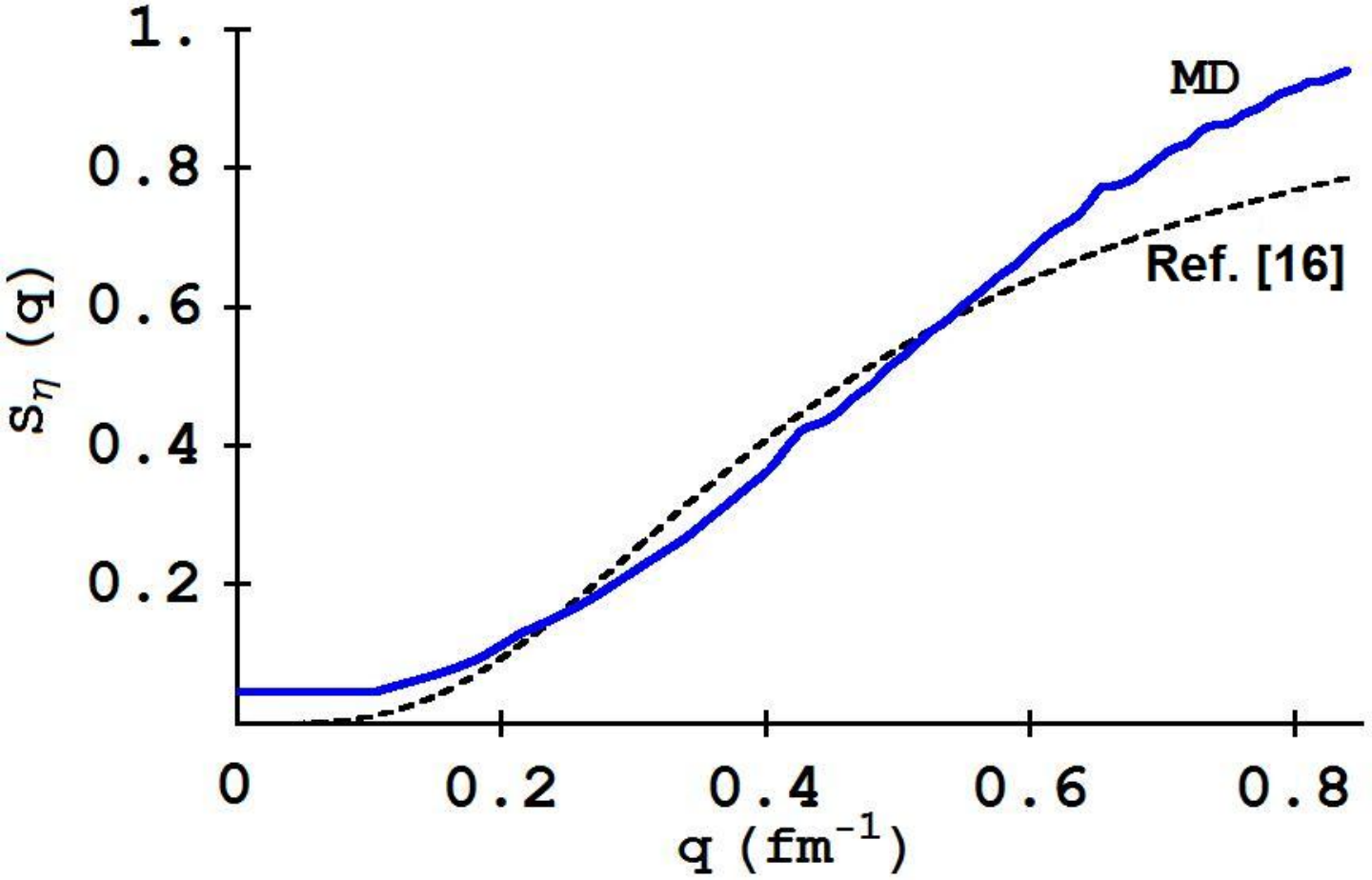
Table 3 shows the viscosity obtained for a simulation with 500 ions at a temperature of 0.1 MeV and an ion density of fm-3. Even with large quantum corrections, the contribution from the ion-ion scattering is small by orders of magnitude compared with the contribution from electron-ion scattering. Therefore, for this regime of densities and temperatures the ion contribution to the shear viscosity of the outer crust in a neutron star is negligible. Nevertheless, the use of MD simulations has allowed us to calculate both contributions.
Our MD formalism can also be used to calculate the thermal conductivity [19]. Again we expect the electron contribution to to dominate over the ion contribution at low magnetic fields. However, large magnetic fields suppress the electron contribution in directions perpendicular to the field; then the ion contribution can be important. For example, Potekhin and Yakovlev [20] find that magnetic fields larger than Gauss can lead to anisotropic temperature distributions. Therefore we expect a field of Gauss to start modifying electron contributions to the shear viscosity. However, it may take significantly stronger fields before the ion contribution to the viscosity dominates that from the electrons.
.
| (fm-3 ) | (fm-3) | (fm-3) |
|---|---|---|
| 0.27 | 26.61 |
VI Summary and Conclusions
We have calculated the ion contribution to the shear viscosity in the outer crust of neutron stars. We use two different methods for this purpose. One of these is based on MD simulations while the other is semi-analytical and calculates the transport cross sections for classical and quantum systems. We find good agreement between the two methods in the low density, classical limit.
Using the MD trajectories, we have used autocorrelation functions of the pressure tensor in a Hydrogen OCP to calculate its viscosity. We have studied the case in which the plasma was dilute. In this case the coupling between the ions is weak. We have found that the viscosity is constant at low densities and then becomes an increasing function of density, contrary to the prediction including only binary collisions, where the viscosity remains constant with density. This fact is due to the correlations between ions. The dependence of the plasma viscosity with temperature, at a fixed density, is the one expected for a gas. However, as the temperature decreases changes in the viscosity with density, are larger due to stronger ion correlations.
In the dilute gas limit and for light ion systems, calculations based on the Chapman-Enskog formalism, indicate that viscosities with quantum transport cross sections are nearly a factor of ten larger than the classical results for a fixed screening length of 10 fm. However, for larger more realistic screening lengths, the difference between quantum and classical calculations is smaller.
Using the structure factor of the ions we calculate the contribution to the shear viscosity due to electron-ion scattering. We find that the contribution to the shear viscosity from the ions is negligible compared to the former one for the conditions of interest in the outer crust of neutron stars. Therefore, we do not expect major damping of the r-modes from the ions in the crust.
Our method of calculating the electron contribution via the structure factor of the ions also allows us to use multi-component plasmas, and the contribution of electron-impurity scattering will be automatically included. On the other hand, we have used ion autocorrelation functions of the pressure tensor, and the Kubo formalism to calculate the viscosity of the ions. This method could be extended to calculate other mechanical properties of the ions, like the shear modulus, of great importance in the understanding of starquakes.
Acknowledgements
The research of O. L. C. and C. J. H. was supported in part by DOE DE-FG02-87ER40365 and by Shared Research grants from IBM, Inc. to Indiana University. The research of S. P. and M. P. was supported by the Department of Energy under grant DE-FG02-93ER40756.
Appendix. Calculation of the phase shifts
Here, we employ an efficient algorithm proposed by Klozenberg [21] to calculate the phase shifts. The radial part of the Shrödinger equation is
| (28) |
where is the reduced mass, is the separation distance, is the angular momentum quantum number, is the wave number such that energy and is a spherically symmetric potential. Two new functions and are defined through the relation
| (29) |
such that
| (30) |
where and are the Ricatti-Bessel functions, the solutions of the free radial equation (28) when .
With the function , Eq. (28) becomes
| (31) |
Let us introduce the dimensionless variable and write Eq. (31) as a phase equation
| (32) |
where . By the construction in Eq. (29), the tangent of the phase shift is the limiting value of
| (33) |
where the existence of the limit is assured by the fact that the potential falls sufficiently rapidly as . When the phase shift is close to plus multiples of , we consider the function and its differential equation
| (34) |
to avoid large values of and its infinities. To treat the singularities associated with the Ricatti-Bessel functions when , the normalized analogues
| (35) |
are used with the corresponding equations
| (36) |
| (37) |
To find the initial conditions, let us expand the solution of Eq. (36) around as
| (38) |
and assume that the expansion for is known and has the form
| (39) |
This leads to the coefficients
| (40) |
| (41) |
whence
| (42) |
which is the initial condition for Eq. (36). During numerical integration, we switch to Eq. (37) when , and if we return back to Eq. (36). This procedure is carried out until reaches unity, when we switch to the set of Eqs. (32) and (34). After the solution reaches its limiting value of in Eq. (33) to satisfactory precision, the evaluation is stopped.
JWKB phase shifts
The JWKB approximation allows fast and simple calculations of phase shifts for large and moderately large -values. Here we briefly describe this method following Mott and Massey [22], and, Cohen [23]. Let us write the wave equation as
| (43) |
| (44) |
If the particle’s energy and angular momentum are sufficiently large, such that the potential energy varies only slightly over a few wavelengths, then in the limit we may suppose that is large. Then the solutions of Eq. (43) are approximately
| (45) |
Jeffreys [24] has shown that the solution which decreases exponentially inside the classically accessible region () is
| (46) |
where is the classical turning point given by the positive root of . To find the solution which vanishes as , Langer [25] employed the substitutions and in Eq. (43) and obtained
| (47) |
| (48) |
and by Jeffrey’s method, the solution is
| (49) |
where now .

For large , the asymptotic form of Eq. (49) is
| (50) |
whence
| (51) |
Finally, following Cohen [23], we rewrite the above equation in the form used for numerical evaluations:
| (52) | |||||
where is the classical impact parameter.
For numerical computations, we choose two sets of parameters for the Yukawa potential in Eq. (4): and fm, and, , and fm. An exact calculation of the phase shifts is performed for in the range . For larger values of , up to for and up to for , the phase shifts are computed using the the JWKB approximation. As shown in Fig. 14, the JWKB results are very close to the exact values, even for . The agreement is better for the system with (not shown here), which is essentially classical.
References
- [1] Andersson, N., Astrophys.J. 502(1998) 708.
- [2] B. J. Owen, et. al., Phys. Rev. D, 58(1998) 084020.
- [3] L. Lindblom, B. Owen, S. M. Morsink, Phys. Rev. Lett., 80 (1998) 4843.
- [4] L. Bildsten, G. Ushomirsky, Astrophys.J., 529 (2000) L33.
- [5] N. Andersson, G. L. Comer, Mon. Not. Roy. Astron. Soc. 328 (2001) 1129.
- [6] L. Lindblom, G. Mendell, Phys. Rev. D 61(2000)104003.
- [7] U. Lee, S. Yoshida, Astrophys.J. 586 (2003) 403.
- [8] J. Clemens and R. Rosen, ApJ. 609 (2004) 340.
- [9] A. I. Chugunov, D. G. Yakovlev, Astro. Rep., 49 (2005) 724.
- [10] E. Flowers, N. Itoh, Astrophys. J. 230(1979) 847.
- [11] C. J. Horowitz and D. K. Berry, Arxiv:0807.2603 .
- [12] Kubo, R., Jour. Phys. Soc. Jap., 12 (1957) 570.
- [13] Reif, F.,Fundamentals of Statistical and Thermal Physics (McGraw-Hill, 1965) p. 473.
- [14] S. Chapman, T. G. Cowling and C. Cercignani, The Mathematical Theory of Non-Uniform Gases, Cambridge University Press, 1970.
- [15] E. A. Uehling, Phys. Rev., 46, (1934) 917.
- [16] A. Y. Potekhin, D. A. Baiko, P. Haensel and D. G. Yakovlev, Astron. Astrophys., 346 (1999) 345.
- [17] Jancovic, B., J. Stat. Phys., 17 (1977) 357.
- [18] N. Itoh, S. Mitake, H. Iyetomi and S. Ichimaru, Astrophys. J., 273 (1983) 774. Systems (McGraw-Hill, New York,1971).
- [19] C. J. Horowitz, O. L. Caballero, D. K. Berry, arXiv:0804.4409.
- [20] A. Y. Potekhin and D. G. Yakovlev, Astron. Astrophys., 374 (2001) 213.
- [21] J. P. Klozenberg, J. Phys. A:Math., Nucl. Gen., 7 (1974) 1840.
- [22] N. F. Mott and H. S. W. Massey, The theory of atomic collisions, (Clarendon Press, 1965, Oxford), Chapter V.
- [23] J. S. Cohen, 1977, J. Chem. Phys., 68 (1977) 4.
- [24] H. Jeffreys, Proc. London Math. Soc., s2 23 (1925) 428.
- [25] R. E. Langer, Phys. Rev., 51 (1937) 669.