![[Uncaptioned image]](0807.4329v1/uabft.png)
Ph.D. Thesis:
Can the PVLAS particle be compatible
with the astrophysical bounds?
by
Javier Redondo
Bellaterra, 2007
Preface
Very recently, the PVLAS collaboration has reported the observation of two unexpected effects. Studying the propagation of linearly polarized laser light through a strong transverse magnetic field in vacuum they find an anomalous rotation of the polarization plane as well as an induced ellipticity of the outgoing beam. None of these two effects has a standard explanation within conventional physics at this moment, but they converge into a frequent prediction of physics beyond the standard model of particle physics: the existence of neutral and nearly massless bosons coupled to light.
The key word in the above paragraph is “unexpected”. Indeed, the small collaboration was actively looking for these so called axionlike particles (ALPs) leading to the two mentioned effects. The important point is that these particles seem to have couplings to the electromagnetic field which are far to be allowed by other experiments and, in particular by astrophysical arguments.
A conservative look would then discard immediately the ALP interpretation of the PVLAS signal but I shall show in these few pages that this decision would be a bit premature. In these years under the supervision of Dr. Massó we have showed that there are particle physics models in which the discrepancies coming from astrophysics and other laboratory experiments can be circumvented. Notably, these models involve new physics at low energy scales. In this PhD thesis I address the issue of presenting all our conclusions.
The realization of this work has been a great pleasure for me, in part because of the confluence of the many fields of physics involved, optics, astrophysics, cosmology and, of course, particle physics, but mostly because it has been carried out in friendly touch with many experts on all these fields. It has been then twice an enriching experience also, but moreover, I think that has given our work a soundness which otherwise would be lacking. The multidisciplinarity of this thesis has a natural drawback, however, one would be tempted to review all the fields involved and produce a too long writing. I was not really seduced with this idea and I have tried only to touch the points I really consider important to understand my original work. Wherever I feel there is more to be said I give the needed references.
Since the publication of the PVLAS result we have been witnesses of a real “boom” in the field with both, theoretical efforts and the advent of many experimental proposals to test the PVLAS ALP interpretation. This reflects, among other things, the great importance of having new tests of physics beyond the standard model. In the years before the Large Hadron Collider, which will scan TeV energies with an unprecedent budget in the history of physics, we could be finding a new frontier of knowledge in a much more modest experiment, and at very low energies.
In Chapter 1 I briefly motivate low mass particles coupled to light and introduce the required ingredients that will show up in my models. I am concerned with scalar particles such as pseudoGoldstone bosons, candidates for the PVLAS ALP, paraphotons and millicharged particles. Chapter 2 is devoted to introduce the PVLAS experiment as well as its ALP interpretation in terms of a new scalar particle coupled to two photons. Further comments will be made about other possible interpretations. Finally, in Chapter 3 I review the experimental knowledge about the low mass particles coupled to light that could be involved in the PVLAS signal and state the inconsistency of the bare PVLAS ALP interpretation with astrophysics and two very sensitive experiments: ALP helioscopes and 5th force searches.
Chapter 4 constitutes an introduction for the original work presented in this thesis. My contributions are organized as a compendium of articles published between the years 2005 and 2007, each in a separate Chapter. The chronological order in which they appear reflects somehow the evolution of the theoretical efforts required during these last three years. Chapter 5 (reference [1]) gives two general ideas for reconciling the ALP interpretation of PVLAS with the physics of stars introducing new particles and interactions at low, accessible, energy scales eV. The concrete models proposed seem to be now a bit obsolete but the message imprinted remains valid, there is need for additional low energy physics in order to evade astrophysical bounds on the PVLAS particle.
A further refined model is presented in Chapter 6 (reference [2]). There we include two paraphotons and a millicharged particle, together with the PVLAS ALP, in order to circumvent the astrophysical constraints. The model is simple and, although it has some fine-tuned quantities, turns out to be one of the few models that could to the job if the PVLAS ALP is confirmed.
Even before the time this paper was published, the community was starting to be active proposing other models and we had the feeling that some model-independent study of evading astrophysical bounds could be of interest. Therefore we prepared [3], which is presented in Chapter 7, as a tool of evaluating more precisely the models in [1, 2] (which lack precise calculations) as well as any other of similar characteristics11 1 Interestingly enough, we noticed a new way of evading the astrophysical bounds if the PVLAS particle is a Chameleon field.. The general conclusion is again that the new physics should appear at scales accessible for Earth-ground laboratory experiments (even lower than naively expected) and therefore experimental efforts were strongly encouraged.
Last summer, the PVLAS collaboration released new data suggesting the parity of the ALP. Measurements performed in gas indicated that the ALP should be a parity-even particle and therefore it would mediate long range forces between macroscopic bodies. In the last article presented in this thesis (Chapter 8 from reference [4]) we analyzed such a possibility. The very precise measurements of the Newton’s law and Casimir effect rule out contributions of the PVLAS particle and the impact in the parameter space of ALPs is really impressive. Moreover, we realized than in the model presented in Chapter 6, the force is suppressed with respect to the naive expectations and the ALP interpretation of PVLAS is possible.
Finally, In Chapter 9 a short summary and a final discussion are presented.
Chapter 1 General concerns about light weakly coupled particles
1.1 Introduction
Despite the considerable success of explaining almost every observation within particle physics, the standard model (SM), based on the gauge symmetry , is generally thought not to be the final theory explaining the interactions between elementary particles. There are several reasons for that, and we can arrange them into three big sets of problems and objections.
The first one is concerned with very fundamental objections to the quantum theory: the postulate of measurement, the lack of a direction of time, etc. The second is less fundamental and simply concerns the elusion of the gravitational interactions. This problem is addressed at present within quantum gravity and string theory, being the last the most promising but still far from providing mature answers.
Finally, the third set are problems regarding the concrete form of the standard model as a quantum field theory. Most of them can be regarded as purely “aesthetical” features. As examples we find the large number of parameters (coming from our ignorance of a possible flavor structure at higher energies?), the flavor problem (why three generations?), the hierarchy problem (why such a difference between the electroweak (EW) and the Planck scales?), the missing Higgs boson (where is it?), the strong CP problem (why does QCD respect CP?), etc.
While the first two sets of “fundamental problems” of the SM seem difficult to solve in a quantum field theory framework, those from the third are the subject of many speculative but ingenious proposals beyond the SM. For instance, the existence of a symmetry between bosons and fermions, the so called Supersymmetry, could help to stabilize the EW-Planck hierarchy and theories of dynamical breaking of the EW symmetry do not need a Higgs boson. These models generally introduce new fields and gauge symmetries beyond the SM. Most of the new particles and gauge bosons are extremely massive and we only have chances to discover them by building huge accelerators or by precision measurements of carefully chosen observables.
However there are several of such theories in which also low mass particles are predicted. If these particles exist they must necessarily be very weakly interacting, otherwise they would have been already discovered11 1 This last assertion acts as a definition of “very weakly interacting” and “low mass” in a precise sense.. On the other hand they can be active and stable at the low energies of our universe and give rise to a completely different phenomenology from their massive companions.
This Chapter is devoted to review some relevant scenarios where those particles arise while I leave the study of their peculiar phenomenology to Chapter 3. Particular emphasis will be made on their interactions with the electromagnetic field because these turn out to be specially interesting from the experimental point of view. Indeed many of the experimental efforts looking for these particles have been focused on these couplings, and one of those experiments, performed by the PVLAS collaboration, has recently reported a positive signal.
From a theoretical viewpoint, the existence of low mass particles is closely related to symmetries. Regarding the renormalization group approach, masses are dimensionful parameters of the theory that tend to develop values near the ultraviolet cut-off unless some symmetry forbids them. Put it another way: if we intend to force some dimensionful parameter to be much smaller than the higher energy scale in the theory , radiative corrections involving particles related to will induce contributions proportional to powers of which will have to be canceled at a very precise level with counterterms of the same order. Such a tuned cancelation is generally though to be unnatural and unaesthetical, and it engenders the so called hierarchy problem. The only way to control these radiative corrections is to protect the small scales with symmetries. Indeed, supersymmetric theories were motivated in part to avoid the electroweak-planck hierarchy. As notorious examples we find also the masses of fermions in chiral theories and Goldstone and gauge bosons. Let me say a few words about them.
The lowest-dimension (non trivial) irreducible representations of the Lorentz group in 3+1 space-time dimensions are spinors of left and right handed chirality. Parity transformations convert one set into the other but, although parity is approximately conserved, it seems not to be a good quantum number at the most fundamental level. It is allowed then for LH and RH fermions to be in different representations of the gauge group, whatever they are. Dirac mass terms involve just one LH and other RH spinor so they have to combine forming a gauge invariant term. From this viewpoint, a pair of LH and RH fermion fields living in representations that allow a scalar of the gauge group will acquire a mass of the order of the cut-off, , but LH and RH fermion fields which cannot be paired for any reason22 2 For instance, there could be more LH than RH fields in nature, they could belong to representations of different range,etc. would lead to massless modes. On the other hand, Majorana mass terms are allowed only for fields completely neutral under the gauge group. This is the case, for instance, of the RH neutrinos of the standard model which for the above reasoning are supposed to be very massive. Interestingly, a huge Majorana mass for the RH neutrino field produces a suppression of the Dirac neutrino masses by means of the see-saw mechanism.
This picture is valid as long as the gauge symmetry is unbroken. In the standard model, the Higgs field acquires a vacuum expectation value that breaks the sector to . In this way, interactions of Yukawa type of the Higgs with a pair (LH-RH) of fermion fields lead to effective mass terms that are naturally much smaller than the cut-off scale of the theory as long as the vacuum expectation value of the Higgs, or the Yukawa couplings, are small. Explaining why a scalar field like the Higgs could develop a small expectation value GeV (small with respect to the Planck scale GeV) is again the hierarchy problem.
Furthermore, the Nambu-Goldstone theorem tells us that theories with a global symmetry spontaneously broken in the vacuum contain massless particles, known as Goldstone bosons. This result goes beyond perturbation theory so radiative corrections do not spoil this conclusion. Nevertheless most of the known examples of Goldstone bosons come from slightly explicitly broken symmetries which allow for small masses that can be again sensitive to the hierarchy.
Finally, the gauge bosons of a local unbroken symmetry are naturally massless at all orders being their masses protected by the gauge invariance of the dynamics. There is a nice exception in pure symmetries because a mass term is also allowed [5, 6, 7, 8]. From this point of view it seems natural to think that or are not fundamental symmetries but the low energy residual of a higher embedding non-abelian group.
In the remaining of this Chapter I will go deeper into the important theoretical frameworks that provide small mass particles that are crucial for this thesis. I begin with an exposition of the Nambu-Goldstone theorem followed by the related history of two of the most important examples, pions coming from the breaking of the axial part of the isospin symmetry of QCD and axions, Goldstone bosons of a hypothetical broken axial symmetry proposed to solve the strong CP problem. The discussion is focused on this last case, since it has become a kind of paradigm in low mass bosons searches.
Next I consider the phenomenology of new symmetries in a hidden sector, giving rise to paraphotons and millicharged particles. These provide the framework for our solution to the PVLAS-Astrophysics puzzle so I describe them with greater detail.
1.2 The Nambu-Goldstone theorem
The Nambu-Goldstone theorem states that:
whenever a global continuous symmetry of the action is not respected by the ground state, there appear massless particles, one for each broken generator of the symmetry group.
The demonstration of this result inhabits central pages of many text books, so I believe it is not worth to be reviewed here. However, it will prove convenient to express it in mathematical form. To do so, consider the global infinitesimal transformation
| (1.1) |
where are fields (of any type, although only scalar fields are allowed to have nonzero vacuum expectation values), is an array of arbitrary infinitesimals, and are the generators of the transformations with the index running over such transformations. If these transformations are symmetries of the lagrangian there are associated currents which are conserved in the sense that . We can write the Goldstone theorem33 3 I display the result for hermitian and s only for simplicity. as
| (1.2) | |||
| (1.3) |
We see that the Källén-Lehmann spectral density contains a pole in only if the associated symmetry generator is broken in the vacuum, . The corresponding massless particles, known as Goldstone bosons (GB), are created by combinations of the fields that will develop a v.e.v.
| (1.4) |
It is clear that there are as many GBs as broken generators. The contribution of the massless modes to the two-point function (1.2) is proportional to . A nonzero value requires that must be spin-zero fields (because is rotationally invariant) and have the same conserved quantum numbers44 4 The quantum numbers that are conserved also by the vacuum. than (otherwise vanishes55 5 Provided has spin-zero, can not contribute because it transforms as a spin-1 field.).
1.2.1 Approximate symmetries and pseudo Goldstone Bosons.
It is usually the case that global continuous symmetries present in our theories are just approximate. The potential is then divided into a “symmetric” part and a breaking term . If the breaking term is small we also find GB but the new terms can include non-zero (but small) masses. We name such particles pseudo-Goldstone bosons (pGBs). Also, typically, a reduction of the degeneracy of the vacuum configurations is found (the so called vacuum alignment).
1.2.2 Axions and the strong CP problem
Consider quantum chromodynamics with only two flavors of massless quarks, and . The lagrangian of this theory has a global symmetry that allows to perform rotations of LH and RH fields independently, namely
| (1.5) |
where () with the Pauli matrices and free parameters. This symmetry can be also decomposed into vector and axial parts . We can easily associate the part with the isospin symmetry66 6 In the standard model this symmetry is only approximate because and quarks have different electric charge and a “small” mass difference compared with , both due to the electroweak interactions. of the strong interactions. Moreover, leads to conservation of the baryon number, which is an observed property of the strong and electroweak interactions77 7 This is valid up to the electroweak scale where instantons alter the picture..
At first sight there is no symmetry (not even approximate) in nature related to the axial subgroups. At low energies, a quark condensate forms making and thus breaking spontaneously this part of the symmetry. The axial symmetries must then show up in the appearance of the corresponding Goldstone bosons. This seems to be the case for the part because we observe in nature three light bosons, the pions, one for each broken generator of . But there is no such Goldstone boson for the symmetry88 8 The lightest candidate was the , but it turns out to be too big. Weinberg showed [9] that the squared mass of the Goldstone should be smaller than three times the square of the pion mass.. Weinberg stated this puzzle as the problem and suggested that there could be no symmetry in the strong interactions.
The solution of this problem was found by ’t Hooft who realized that the subgroup was indeed badly broken in QCD due to its non-trivial vacuum structure [10]. To understand the main points, first realize that suffers an anomaly due to a triangle loop diagram (Fig. 1.1) with quarks circulating on it. This anomaly contributes to the divergence of its related current with
| (1.6) |
where is the gluon field strength, and is its dual with the total antisymmetric tensor in 4-dimensions. ( is the number of quarks circulating in the loop, in our case.) This itself does not violate because (1.6) amounts a total divergency which in principle could be naively removed (as it happens in quantum electrodynamics)
| (1.7) |

But the surface integral of the Bardeen current can not be set to zero. This is understood when we realize that the QCD vacuum is degenerated being the multiple states gauge transformations of the configuration. They can be classified by the so called topological winding number which characterizes the way these configurations behave at spatial infinity. Notably, the QCD lagrangian allows for non-perturvative solutions of the equations of motion, the so-called instantons that mediate transitions between these vacuum states. But these instantons vanish very slowly at spatial infinity () so they give finite contributions to the integral of the divergence of Bardeen’s current. To be concrete, the contribution of , an instanton taking a vacuum state with winding number to one with is
| (1.8) |
where , the diference in winding numbers. Clearly, is violated by these instantons. This solves the Weinberg puzzle but unfortunately (or not) it poses a new and very interesting discussion remaining nowadays yet unsolved: the strong CP problem.
Note that any physical amplitude must take these instanton solutions into account in the path integral. For reasons of gauge invariance and cluster decomposition one choses a weight factor for any of those configurations. This is formally equivalent to include a new term in the effective lagrangian
| (1.9) |
Such a term violates parity and time reversal invariance but conserves charge conjugation invariance (and thus violates CP). The picture looks a bit more complicated if we take into account that quarks gain a mass after the spontaneous symmetry breaking of the gauge symmetry of the standard model. In general this induces a complex mass matrix
| (1.10) |
( holds for up and down quarks here) that can be diagonalized by a biunitary transformation that involves precisely a rotation (1.5) with
| (1.11) |
This rotation modifies the measure of the quark fields in the path integral of the theory [11] introducing another term like (1.9) in the lagrangian99 9 See the exposition in [12]., shifting the value of and allowing us to define an effective
| (1.12) |
so actually the CP violating term in the QCD sector of the standard model is the sum of two very different contributions, coming from QCD vacuum dynamics and from the electroweak breaking sector. There is no convincing reason why any of these quantities should be zero, and it is even more unlikely that being both non-zero they cancel exactly1010 10 If would have been a true symmetry then this transformation would have had no consequences and the phases of quark masses would be unobservable as well as the term (1.9) which could be rotated away. [13].
However, as mentioned before, a nonzero value of implies CP violating observables related to the strong interactions and, remarkably, it induces an electric dipole moment for the neutron which up to now has eluded detection. The latest measurements [14] set the impressive bound
| (1.13) |
which finally poses the strong CP problem:
why is so small being the sum of two, in principle unrelated, quantities?
Trying to solve the strong CP problem has motivated a lot of work and attractive speculations [13]. Here I focus on the proposal of Peccei and Quinn [15, 16] which has a relevant phenomenological consequence for this work: the introduction of a pseudo Goldstone boson, the axion [17, 18].
Let us first assume a new axial symmetry having a color anomaly . If the symmetry is spontaneously broken at a very high energy (it has to be like this since it is not apparent at low energies) then the low energy effective lagrangian would include a massless Goldstone boson, . Because of the anomaly, develops an interaction term1111 11 We can read it in eq. (1.2) where we see how Goldstone bosons couple their relative currents. This mechanism is the same that provides an interaction responsible for the anomalous decay. For further details see [12].
| (1.14) |
In the rest of the low energy effective theory enters only through its derivatives as a Goldstone boson should. Now, provided that the rest of the theory preserves CP1212 12 CP violation coming from the electroweak sector apart from the quark mass matrix is just a small perturbation to this situation. except the -term (1.9) then the effective potential is even in , having a minimum at which conserves CP. The consequence is that the field develops an expectation value such that is canceled. We can say that the Peccei and Quinn mechanism relaxes dynamically to zero solving the strong CP problem.
Note that the PQ symmetry is almost completely similar to the QCD . The subtle point that makes the difference is that now is a scale much higher than and therefore the instanton effect can be considered now a small explicit breaking of while it was a breaking of . It is because of this reason that the axion exist and the GB of the does not. Due to this small explict breaking, however, the axion acquires a small mass, and hence it is rather a pseudo-Goldstone boson.
Interestingly enough, many of the relevant properties of the axion are independent of the exact realization of the PQ symmetry. For example the field mixes with the neutral pion resulting in two massive eigenstates1313 13 Corrections due to the other mesons are small and irrelevant for this discussion., one very close to and the other called axion whose mass can be easily obtained to be
| (1.15) |
Note also that being an axial symmetry, the axion must be a pseudoscalar spin-zero boson.
Also, the axion field always appears in the lagrangian suppressed by the Peccei-Quinn scale, . The original Peccei and Quinn model set close to the electroweak scale but such a low energy scale was soon excluded. The so-called invisible models [19, 20] propose a much higher value of which makes the axion quite difficult (though not impossible) to detect. Remarkably, the Peccei-Quinn solution to the strong CP problem works independently of the size of this parameter.
Furthermore, it is quite generic that the axion develops a two photon coupling, denoted as
| (1.16) |
with the field strength tensor of the electromagnetic field. The coupling is the sum of two contributions, one coming from a plausible electromagnetic anomaly and the other coming from mixing (See Fig. 1.2)
| (1.17) |
Where is the fine structure constant and is the electromagnetic anomaly of . A cancelation of this coupling is rather unlikely due again to the different nature of the two contributions1414 14 An accidental tuning however is possible in some concrete models. See [21] as a notorious example..

The axion has also couplings to quarks and leptons which have been extensively considered in the literature but, as it will become clear, it is the electromagnetic coupling which has the richest implications nowadays. The phenomenology of this coupling will be the main subject of Chapter 3.
There are beautiful examples of Goldstone bosons other than pions and axions. For instance the so-called Majorons [22, 23] come from the hypothetical spontaneous breaking of the “Baryon minus Lepton” number which was invoked to provide a Majorana mass for neutrinos in a Higgs mechanism fashion. Other celebrated examples are Familons [24], arising from the spontaneous breaking of family symmetries, which are very much related to axions and the strong CP problem.
The general lesson to be learned from this section is that Goldstone bosons arise whenever there is a global continuous symmetry which is spontaneously broken by the vacuum state. If the symmetry is slightly explicitly broken the corresponding Goldstone excitations become massive. Interactions of Goldstone bosons are always suppressed by the energy scale of the spontaneous breaking and involve derivatives except in the case of the anomalous interactions (1.14) coming from the axial anomalies of their corresponding symmetries. The parity and internal quantum numbers of the Goldstone are those of the charge density associated to the broken symmetry.
Quite naturally these Goldstone Bosons can acquire a coupling to two photons through quantum corrections like those giving the anomalies (See Fig. 1.2). But there is one important point to remark here. In what follows I will be considering the phenomenological implications of vertices like (1.16) not restricting myself to the axion case. It happens that they are essentially similar (See Chapter 3) to those coming from the corresponding parity-even gauge field structure
| (1.18) |
which I will consider altogether. There are however important theoretical differences between them. is CP and P conserving (See section 2.3.1) and thus (1.18) respects these symmetries for a CP and P even field . This Goldstone mode is to be originated from the spontaneous breaking of a vector-like symmetry (rather than axial). We know that this is not possible in theories with only vector-like fermions (with non-chiral interactions) like QED or QCD because of the Vafa-Witten theorem [25]. However, this is certainly not a strong restriction; the standard model itself is not subject to it, indeed.
However (1.18) cannot have the same origin than (1.16) since there is nothing like vector anomalies. Put it another way, is not a total derivative. As Goldstone bosons have derivative interactions, (1.18) cannot arise, even for a parity-even Goldstone boson.
These theoretical considerations disfavor somehow parity-even massless scalars coupled to two photons. However (as we saw in the case of the axion) typically global symmetries are not exact and the full effective description of particle physics at low energies will contain terms that explicitly break the symmetry. We know that these terms would provide a Goldstone boson mass so in principle they can also naturally lead to interactions like (1.18).
1.3 Paraphotons and millicharged particles
Extensions of the standard model quite generally contain extra gauge factors. These gauge factors can be fundamental or sit within a non-abelian gauge group. Such gauge symmetries are necessarily accompanied by their corresponding spin-1 massless gauge boson which is automatically a new low energy candidate for new physics.
Gauge bosons can obtain mass from the spontaneous breaking of its related symmetry but purely symmetries allow also for a Stuckelberg mass-term [5, 6, 7, 8]. At the same time there is at first glance no reason for their masses to be small, on the contrary, it is more natural if they are of the order of the highest mass scale in the theory, which it is usually assumed to be the Planck mass GeV. Of course, these arguments do not rule out a small mass-scale, we know at least two completely “unnatural” mass parameters in nature, the electroweak scale ( GeV), and the cosmological constant ( meV).
There are many examples of such particles in the literature: mirror photons, s, shadow photons, U-bosons, etc. They differ in the interpretation that is given to the new symmetry or the way it links with the standard model sector. Here I will refer mainly to “paraphotons”, a term first introduced by Okun [26]. To my knowledge he was the first one to consider these particles, at least in the framework I will discuss here.
On a basic level, the impact of paraphoton models is to proportionate deviations from the predictions of QED, at least at low energies. But also, paraphoton models include naturally millicharged particles, i.e. particles whose electrical charge is not a multiple of the electron charge but a small number1515 15 See the discussion in [27] about charge quantization.. They are, together with paraphotons, necessary ingredients of our solution to the PVLAS-astrophysics inconsistency. Interestingly enough, if the millicharged particles are fermions, they can have naturally small masses in chiral theories like the standard model.
Quantum electrodynamics is usually said to be the most precise theory of all sciences so deviations from their predictions are extremely restricted. This implies that paraphotons and particles coupling to them have to be somehow isolated from our standard particle physics. It has become a fixed tendency to consider that paraphotons and other light paracharged particles coupled to them inhabit a kind of hidden sector. The connection between this and our sector would be then driven by radiative corrections with very massive particles acting as mediators between the two worlds.
Consider a toy model in which we have quantum electrodynamics1616 16 For my purposes it is sufficient to consider how paraphoton models alter the standard QED scenario. A wider scope would consider the whole standard model [28]. in our sector (labeled ) and a similar theory for the hidden sector (labeled ). The complete gauge symmetry is then and the gauge piece in the lagrangian is the sum of two similar parts
| (1.19) | |||
plus a term that mixes kinetic terms of the gauge bosons
| (1.20) |
where are the field strength tensors of the gauge bosons , are the respective gauge couplings and are the -charges of the different fermions . We are interested in models in which there is isolation of the 0 and 1 sectors so I put the tree level term (1.20) to zero at zeroth order1717 17 There are two natural ways to obtain this: let sit within a non-abelian gauge group and the tracelessness of its generators will ensure , alternatively consider a discrete symmetry at high energy broken for instance by fermion masses at lower scales. Both cases have been discussed in [29]. and consider that the masses of mediators, fermions charged under both ’s (’s) are very high so they can be removed from the low energy physics.
Although decoupled, these fermions (of mass ) lead to a small correction1818 18 Other radiative corrections produce the usual charge, mass and field strength renormalization which do not interfere with my conclusions here. to through the diagram depicted in Fig. 1.3
| (1.21) |

The dimensionful logarithm is understood to be regularized in any of the standard ways but a simple choice of the charges of the heavy fermions can evade this complication. For instance, I can choose two fermions, and , to get . If one does not assume a fine cancelation due to mass degeneracy and use , the obtained value is of order . However one expects indeed higher degrees of symmetry and degeneracy as the energy scales involved (here the masses) are increased and thus it is “natural” to obtain much smaller values for for example in supersymmetric models or in string theory [29].
We call the “interaction basis” of the gauge bosons because the interactions with their relative fermions are diagonal by definition. In opposition to this we can find a “propagation basis” in which (1.20) is rotated away and the gauge fields are eigenstates of propagation. In the course of diagonalizing the kinetic gauge sector we are led with mixed charge assignments. Then, in our calculations, mixing terms can be traded for off-diagonal charges, a fact that I reviewed in [30, 31] in the context of the model proposed in [2] solving the PVLAS-Astrophysics puzzle (Chapter 6). This can be shown in two ways, either by direct diagonalization of the kinetic part of the lagrangian or by studying the elastic scattering amplitude. Let me show both of them.
1.3.1 Diagonalization of the kinetic matrix
First write the kinetic part of the lagrangian in a matrix form, adding a general mass term that will prove to be very convenient later on
| (1.22) |
Where are vectors with components and Lorentz indices have been suppressed. I choose the mass matrix to be diagonal in the interaction basis since it is more likely that this mass is gained through interactions, then
| (1.23) |
To diagonalize and express the result in canonical form we perform a rotation of followed by a contraction (). In the resulting basis, is not diagonal but it is symmetric so a further rotation is able to diagonalize it also ( Diag). The matrix transforming from the “interaction” to the “propagation” basis is therefore and takes a very simple form when we consider the interesting asymptotic case
| (1.24) |
The fermion interaction in this basis acquires the promised non-diagonal charges. For instance, we get a -sized electric charge for the paracharged fermion
| (1.25) |
and a small paracharge to standard model charged particles, for instance electrons , with , implying
| (1.26) |
The massless case is special. The freedom to choose the matrix becomes an arbitrariness of the definition of the propagation basis and thus of the charge assignments. It is conventional then to define the propagation photon along the direction of the interacting photon so standard model charged particles, ’s, do not interact with the resulting paraphoton but parafermions acquire an -sized electric charge. In this case we have
| (1.27) |
However, this is nothing but a definition without physical meaning. We could also have chosen a situation in which standard model particles have paracharges, or even a mixed situation. I have found that one can get the most general result from (1.24) performing the limit ending up with
| (1.28) |
for arbitrary as long as to ensure that the off-diagonal elements of (1.24) are always small.
It is interesting to note that one cannot get this result by putting into the corresponding and letting . Although seem to imply also a rotational freedom, a small -sized mass difference arises in the propagation basis breaking the rotational invariance (This mass difference is proportional to so this does not spoil the freedom in the massless case.).
In general , etc. will differ from the interaction values in small -sized quantities.
1.3.2 scattering amplitude
The charge assignments of the last subsection can also be obtained in a very simple calculation, a procedure that turns out to be much simpler in models involving several paraphoton fields (I will need two of them for my purposes). Consider the elastic scattering amplitude of a -fermion with a fermion, by using the mixing term in (1.20) as an interaction (It can be done provided is small)
| (1.29) |
( is the 4-momentum carried by the bosons, the currents of particles and I have used ) which we can decompose using
| (1.30) |
This amplitude is equivalent to the sum of two single boson exchange diagrams as shown in Fig.1.4, which require that we assign an -charge to and a -paracharge to :

| (1.31) |
We naturally associate these intermediate bosons with the propagation states we calculated before, and we find (always at first order in the small quantity ) from (1.19),(1.24) and (1.31) that, as expected, both approaches give identical charge assignments.
The diagram studied, however, does not give us information about the values of the order corrections to . To calculate them we shall study or elastic scattering. In that case, beyond the order diagram in which the two electrons (s) interchange a () there is another contribution in which the () intermediate state turns for a while into a () to reconvert again into the original “flavor”. These diagrams provide the corrections to the masses and gauge couplings.
1.3.3 Some remarks
First note that only particles charged under will receive a -sized charge of type and viceversa. Neutral particles as the neutrino will continue being completely neutral if photons mix with a new gauge boson from a given sector. Notably this holds for composite “states” as for instance atoms. Also, notice from (1.26) that for instance, electrons will gain an opposite paracharge than protons because their charge is opposite.
Second, note that the matrix (1.24) is not unitary, reflecting the fact that “interaction” states are not orthogonal, since they have a kinetic mixing term. Such a complication does not make difficult the calculation of the oscillation probability. If we prepare states using (1.24) their temporal evolution will be easily expressed in the propagation basis
| (1.32) | |||||
| (1.33) |
where is the energy of the state and I have not taken into account the normalization, irrelevant for the following computation since it just provides terms. We find
| (1.34) | |||||
| (1.35) |
Where for the relativistic limit . We see clearly that in addition to the typical oscillation sinus, a contribution has arisen, due to the fact that has a small component along (another way of looking at the mixing term) of size . This is made clear in Fig. 1.5.
Another interesting difference with neutrino oscillations is that in the case , there are no oscillations, even if . This situation corresponds to one where and then so clearly no oscillation could happen since one of the “interaction” states is a “propagating” one, namely .

It is common to consider experiments of disappearance of photons (), as for instance light-shinning-through-walls experiments (See subsection 3.3.3). It will prove useful then to define the sterile states , as the states orthogonal to the interaction ones . The probability of oscillations is therefore derived in complete analogy to the neutrino oscillations case to be
| (1.36) |
These sterile states were called ”paraphotons” by Okun [26] although here we have used the name for a general abelian gauge boson. It is mandatory to compare this construction with the original work of Okun [26]. There are two main differences. First, he did not consider a current of type . Second, he did not wonder where do the mass terms come from. In my work I need particles charged under the hidden sector gauge group , but most importantly, I assume that the mass terms come from interactions within the two gauge groups separately, i.e. the interaction states have a diagonal mass matrix.
Chapter 2 The PVLAS experiment
2.1 Introduction
A photon can convert into a neutral boson in an electromagnetic field in the presence of a interaction. This is the so-called Primakoff conversion first proposed by Henry Primakoff to measure precisely11 1 In this case they use the Coulomb potential generated by an atom as the electromagnetic field. the decay constant [32].
Moreover, if the particle is light enough, this vertex would lead to “mixing” where a coherent superposition of the two particles arises, in complete analogy to the -meson or neutrino systems. Notably, in this case and due to the presence of the magnetic field, the angular momentum needs not to be conserved, allowing the mixing of photons with particles of higher (but integer) spin.
This immediately suggests a possibility for looking for novel bosons coupled to light in a classical optical setup. Consider Fig. 2.1., a photon from a laser beam interacts with an external magnetic field and it is converted into a boson. If this absorption is selective, i.e. is different for photon polarizations parallel () and perpendicular () to the magnetic field direction, the vacuum permeated by magnetic fields would act exactly as a dichroic medium since both polarizations will be depleted at different rates. The net effect on a polarized beam will be a rotation of the polarization plane which can be measured. This can be seen in 2.1., where I depicted a view of the plane perpendicular to the laser direction showing in and out polarizations of the incoming laser. It is straightforward to see that the sign of the rotation will be positive if the coupling favors transitions and negative in the opposite case. As we will see, the sign of the rotation will be used to determine the parity22 2 More precisely the parity structure of the two-photon part of the interaction. of .
Maiani, Petronzio and Zavattini were the first to realize that the two photon coupling of low mass bosons (in fact they considered only spin zero bosons) also leads to birefringence for light propagating in strong magnetic fields [33]. The boson can be produced and, after some distance, reconverted33 3 This can happen even off-shell, i.e. with 4-momentum squared different to . as shown in Fig 2.1. resulting in a phase delay of the photon. Again, if transitions are more likely than or viceversa there would appear a phase difference between the two polarizations and then the outgoing beam would show a counter-clockwise or clockwise ellipticity (See Fig. 2.1.). We can conclude then that the vacuum permeated by magnetic fields would behave as if it were a dichroic and birefringent medium.

Indeed it was known long ago (See [34] and references therein) that pure QED effects already produce birefringence in a transverse magnetic field in vacuum (a vacuum Cotton-Mouton effect). This is due to virtual electron loops like the one depicted in Fig. 2.2 which lead to the following indices of refraction [34]
| (2.1) |
| (2.2) |

It was T. Erber [35] the first to propose the use of a polarized laser beam propagating in a magnetic field to measure the vacuum QED effects. However, he was wrong thinking that it leads to a rotation of the polarization plane, not to an ellipticity. Some years after Iacopini and Zavattini [36] wrote an interesting experimental proposal44 4 Apparently unaware of Erber’s idea. to detect this ellipticity at CERN. Time passed by and the paper of Maiani, Petronzio and Zavattini [33] came out supporting the idea of such an experiment55 5 Little time after, Raffelt and Stodolsky [37] showed that this paper contained some overestimated predictions. They had claimed that they would be able to measure the QED birefringence effect and values of GeV-1, competitive with the strong astrophysical bounds. with the possibility of detecting low mass bosons coupled to light (at a time in which axions and other light bosons like arions [38], majorons [22] or familons [24] were very fashionable).
Finally, a pioneer experiment was performed in the Brookhaven laboratory by the so-called66 6 From Brookhaven, Rochester, Fermilab and Trieste, homeplaces of the members of the collaboration. BRFT collaboration. They found no signal of this kind of interactions77 7 This experiment, as we will see, was also sensitive to the existence of paraphotons. [39, 40] so they were able to establish exclusion bounds on the ALP parameter space. Most of the collaboration moved then to the National Laboratory of Legnaro, near Padova (Italy), where, under the leadership of E. Zavattini, they started to build the PVLAS experiment [41] as a natural continuation of the BRFT apparatus and technique. Next I will comment on its set up to end up with their latest results.
2.2 PVLAS experimental setup and recent results
The PVLAS experiment is as simple as beautiful. The basic idea consists in sending a laser beam along a strong transverse magnetic field located between two crossed polarizers, all in a cavity at high vacuum, see Fig. 2.3. It is clear that if light does not interact with , then no light would came out from the second polarizer. Conversely if the magnetic field in vacuum has optical properties such as dichroism or birefringence then the situation would change and some emerging light would “enlighten” the phenomenon.

As I mentioned this should be the case if one takes into account quantum fluctuations of the QED vacuum structure, producing a net birefringence but no dichroism. Also, in the case that a light boson with a two-photon coupling exists, the real and virtual production shown in Fig. 2.1 will lead to both a rotation and an ellipticity of the outgoing beam.
In the PVLAS experiment the magnetic field intensity reaches T and the length of the magnet is meter. With these parameters, the two perpendicular components of light emerging from the magnetic field would have accumulated a QED-induced phase shift from (2.1) implying an ellipticity88 8 Ratio of the minor to the major axis of the polarization ellipse shown in 2.1.d. See section 2.3.3. of which means that only a ridiculous amount of light will traverse the two polarizers. Even using a MegaWatt laser (which probably would destroy the polarizers), the emerging light would be far beyond the reach of any present (and maybe future) photodetector.
For this reason, the PVLAS signal is enhanced in two different ways. First of all, the magnetic field is located inside a pair of highly reflective mirrors (actually a Fabry-Perot cavity) which increase the path of light through the magnet by a huge factor . This might look quite a cheap way of building a km length magnet, but it is not exactly the case as I will show below. Second, the outgoing signal is enhanced by heterodyne combination with an ellipticity modulator (called SOM for Stress Optical Modulator) before entering the detector. The principle of heterodyne detection is very simple, two waves at frequency and traveling through a non linear material will produce outgoing waves at frequencies . The amplitude of these waves depends linearly on both amplitudes of the incoming waves. This trick can be used to amplify a very small amplitude by combining it with a larger one and look at any of the interference waves. This procedure, however, demands that the small incoming wave to detect (with our desired excess ellipticity) is beating at some frequency99 9 The original setup in [33] used a modulated Faraday cage. PVLAS is nowadays involved in the modifications required to implement this other technique as a crosscheck of their results. and in order to do so, the PVLAS collaboration managed to make the magnet rotating at a small frequency1010 10 The angle twisted in the photons-time-of-flight is a ridiculous rad. Hz.
The whole resulting setup is depicted in Fig. 2.4 and is able to measure ellipticities as small as rad Hz. This setup can be adapted very easily to measure rotations because a properly oriented quarter wave plate transforms small rotations into ellipticities and viceversa [42], so if placed just before the SOM it will convert a possible rotation generated by the magnetic field into an ellipticity which will be again enhanced by heterodyne combination in the SOM and thus detected. Also, interchanging the slow and fast axis of the quarter wave plate produces a sign flip in the outgoing ellipticity, providing a check of the nature of the signal detected.

With this setup the PVLAS collaboration has recently reported [43] an excess rotation of rad/pass for laser light of nm traveling through a m length, T, magnetic field. This signal has been reported after careful search of possible systematic effects1111 11 For a review see [44] over several years. Also they have reported in several conferences [45, 46, 44] positive results for the search of birefringence, again at the rad/pass level. This amazing result exceeds by three/four orders of magnitude the QED expectations and nowadays remains without a conclusive explanation within conventional physics.
However, there are two non standard candidates that in principle could account for the PVLAS results within particle physics. The first one is a neutral boson weakly coupled to two photons, one of the original motivations of PVLAS. Such a particle will be called from here on axion-like particle (ALP). I devote next section to examine this possibility.
The second possibility has arisen very recently [27] and assumes the existence of very light millicharged particles (MCP). Again, the reactions distinguish both photon polarizations and will lead to dichroism and birefringence.
A very interesting paper has recently appeared comparing both ALP and MCP scenarios and it seems that we will have to wait until more experimental data is released to decide which of them, if any, is more likely to be the responsible for the PVLAS signal [47].
Both explanations have many things in common however, the first one being that they are not satisfactory at all because they are excluded by astrophysical arguments, as I will show in Chapter 3.
But moreover, they share a much more interesting feature, both scenarios can be made compatible with astrophysical observations within a concrete model I presented in [2] and constitutes the central work of this thesis.
2.3 Axionlike particle interpretation
The study of coherent oscillations in presence of a long, static homogeneous magnetic field has been addressed by many authors [33, 37, 48, 49]. Here I follow the exposition of Raffelt and Stodolsky [50].
I do not feel the necessity of including the effects of the QED vacuum since they are very small compared with the PVLAS signal. But it is worth to recall that any birefringence will show up into a rotation when the magnetic field rotates (as in the PVLAS setup) [51, 52]. Nevertheless, it is quite intuitive (and has also been proved rigorously in [52]) that these effects are negligible for the PVLAS setup1212 12 The attempt made in [51] to explain the PVLAS signal in these terms is mistaken.. In what follows I neglect the rotation of the magnet.
Consider the following situation. A beam of laser light is shone against a region where there is a strong magnetic field. I choose the beam direction as the z-axis and the magnetic field polarization to lie in the xz-plane. It is convenient also to make the problem one-dimensional, in the sense that all fields we want to determine are functions of time and only.
| (2.3) |
This is formally the case if the magnetic field would be infinite in the directions and the laser is described as a plane wave. Effects from deviations of this simplistic picture are small.
Next, I consider that there is an interaction between two-photons and a new neutral boson, called , which is very light (we will see soon how light this “light” means). The most discussed case is that represents a spin-zero particle, but also one might consider that is a spin-1 particle like a paraphoton or a spin-2 particle like the graviton.
In Chapter 1 we have found motivations for two different couplings associated with opposite parity structure (1.16) and (1.18) which I rewrite here for completeness
| (2.4) |
We know that parity is not exactly conserved by the weak interactions so there is no strong reason a priori to think that it should be conserved by new additional interactions. This suggests not to either assign a definite parity to nor to remove one of these two interactions. However, if is a true Goldstone boson then it could easily happen that it has a definite parity. Explicit breaking terms can modify this statement, but corrections should be small and then one of the ’s will be much smaller than the other. Moreover, unless and are fine-tuned1313 13 Maximal parity violation in a hidden sector like this might not propagate to the SM sector and thus it should not be excluded at first glance. these considerations will not change our main conclusions. This holds also for the case in which there is more than one neutral boson .
It is then enough to consider only one of the two interactions. Following criteria of theoretical and historical importance I choose the parity-odd interaction which arises for axions and other celebrated pseudo Goldstone bosons and drop the sign of the coupling for simplicity.
The lagrangian for the system is1414 14 In all this thesis I am using the metric .
| (2.5) |
whose equations of motion are
| (2.6) | |||||
| (2.7) |
where I have included the electromagnetic current . We can divide the field strength into two parts corresponding to the external magnetic field (with the definition1515 15 This is not a “local” statement. A far away generates the magnetic field at the region where the laser is shinning by contour conditions. ) and the laser beam,
| (2.8) |
If we consider that the external magnetic field is much more intense that the laser beam we can neglect terms involving two fields, and to find a linear system of two coupled second order differential equations
| (2.9) | |||||
| (2.10) |
Note that this is the case in the PVLAS experiment, since and the laser power is mWatt in a mm diameter gaussian beam which means (taking into account the Fabry-Perot cavity which enhances by a factor because the coherence of the reflections.) Then the wave equation for the time-varying potential (in Coulomb gauge ) is
| (2.11) | |||||
Where is the transverse part of the external magnetic field (). As the coefficients of the unknown fields are time independent it is natural to guess a solution of the form
| (2.12) | |||||
| (2.13) |
which implies
| (2.14) | |||
Recall that the electric field will be . For simplicity in further expressions I will evade imaginary quantities redefining .
The solution of the first equation is trivially a plane wave with momentum . In the coupled set we can made a further approximation if the photons and are very relativistic, in this case . The resulting equation is therefore of first order and easier to solve
| (2.20) |
The solution reads
| (2.21) |
being the mixing matrix in (2.20). To get a useful expression for we must diagonalize with a rotation of an angle defined by
| (2.22) |
The resulting states are eigenstates of propagation because for them the evolution is decoupled
These solutions carry momentum and and invariant masses and . When we specify the initial conditions for we find
| (2.31) | |||||
| (2.32) |
In order to get formulas for the probability of appearance of particles and disappearance of photons, we interpret these fields as probability wave functions. Then we find the probability of oscillations at a distance and time
| (2.33) | |||||
| (2.34) |
with
| (2.35) |
The typical oscillation pattern arising from these formulae is shown in Fig. 2.5. In order to maximize the signal there is an optimum distance at which to place the detector at , with an integer.

l
There are two very interesting limits of these expressions, the weak and the maximal mixing limits.
Weak mixing limit, .-
In this case and the
corresponding eigenstates of propagation are very close to the original
| (2.36) | |||
| (2.37) |
We also can expand the square root of the diagonal elements of to find that at first order
| (2.38) | |||||
| (2.39) |
also very close to the original photon and . To get the results usually quoted as the ‘‘weak mixing” limit, one has to assume also that1616 16 An observation which it is not usually done. , then we obtain
| (2.40) | |||||
| (2.41) |
Interestingly enough this weak mixing limit applies in the case of the PVLAS ALP parameters since for T, eV, GeV, meV we find
| (2.42) |
Maximal mixing limit .-
In this case , implying . The corresponding
eigenstates and eigenvalues are
| (2.43) | |||
| (2.44) |
| (2.45) | |||||
| (2.46) |
| (2.47) | |||||
| (2.48) |
Note that in the limit there is no imaginary part, as expected from the fact that it comes from the difference in the propagation speed of photons and ’s of the same energy, which vanishes for . Still there is a real part that provides transitions. This is an opposite situation to neutrino oscillations because here the oscillations are driven by the interaction and not by mass mixing.
Regarding the formulae for we see that the limits in maximal and weak mixing coincide. However, for long distances the maximal mixing formula (2.48) can grow until while the weak mixing result (2.41) has a small maximum value. These results will show their interest later on, when I consider the possibility of measuring oscillations in a low pressure gas. There we will find that controlling the gas pressure we can effectively set and get this maximal mixing situation.
2.3.1 Parity arguments and parity-even ALPs
It is quite remarkable that the set of equations (2.11) decouples into two sub-sets, (2.14) and (2.3). This can be understood with parity arguments as shown in [37]. Instead of using P let us define the parity transformation1717 17 This is nothing but the conventional parity P, with a further rotation of 180o in the plane. as
| (2.49) |
Where now I denote as the coordinates projected onto the plane containing the magnetic field and the direction of the laser beam (the plane) and the orthogonal direction (the axis). Then, electric and magnetic fields transform according to
| (2.50) |
where again refer to the vector components in the plane and along the perpendicular direction . This can be easily seen if one considers how and change if we apply this transformation to a charge or a current distribution (See Fig. 2.6). Moreover the charge conjugation operation changes sign of both electric and magnetic fields , . The external magnetic field changes sign under both C and so is left invariant under the combined transformation . Finally, also the ALP interactions (2.4) can respect this symmetry. The pseudoscalar interaction can be written in terms of the electric and magnetic fields
| (2.51) |
which at the view of (2.50) is invariant when is CP∗-odd, i.e. if is P-odd1818 18 The field is neutral so C and scalar so invariant under the rotation added to P∗ . Conversely, the scalar interaction is written
| (2.52) |
and will be CP∗ invariant for a P-even field.
In any of these cases, the whole dynamics is invariant under CP∗ and thus the eigenstates of the system can be classified by the eigenvalues of CP∗. Therefore, at the view of Fig. 2.7, we can conclude that:
-plane waves are CP∗-odd and -plane waves are CP∗-even1919 19 This is true even if some small longitudinal component arises in a medium.. In the presence of Parity conserving interactions they can only “mix” with particles of the same parity.


Splitting (2.52) and (2.51) into the external magnetic field and the laser contribution we get :
| (2.53) |
| (2.54) |
where for the last equality I have used for a plane wave in vacuum. At this point we understand that starting with the parity-even structure (1.18) we would have ended up with exactly the same system of equations (2.11) interchanging the role of and states. Finally, (2.31) and (2.32) hold as the solutions for and a parity-even- mixing with the coupling (2.52).
2.3.2 Angular momentum conservation
It is also is interesting to note that only transverse magnetic fields are capable of inducing transitions between photons and spin 0 particles. In order for these transitions to occur, the “mixing agent” (the external magnetic field) has to match the quantum numbers, in this case the spin component .
Formally we can write the external magnetic field as proportional to the angular momentum operator and consider the transition amplitude. Using for the photon eigenstates of with eigenvalue we find that
| (2.55) |
by conservation of the total angular momentum. So a longitudinal magnetic field () cannot mediate such transitions, although allows transitions between and states, as occurs in the Faraday effect to be discussed later on.
Finally, I have also considered together with E. Massó and C. Biggio the case in which is an spin-2 particle [53]. In this case we have explicitly checked that a transverse field can mediate transitions between photons and states while a longitudinal one will be responsible for the transitions to .
2.3.3 Rotation and ellipticity
A general light wave propagating along the -direction can be parameterized by means of the Stokes parameters defined by
| (2.56) | |||
| (2.57) |
Where the electric field is .
From them it is easy to derive the formulae for the angle of polarization , the ellipticity angle , and the ellipticity , of a generically polarized plane wave
| (2.58) |
The physical interpretation of these quantities is made clear in Fig. 2.8.

We can parameterize a small change in amplitude and in phase as
| (2.59) |
and let be small real quantities, for which we can use .
Then, if the initial beam is linearly polarized at angle (See Fig. 2.1.a ), after passing the magnetic field it shows a rotation of the polarization plane2020 20 We see here how if the magnet is rotating “adiabatically” (), as in the PVLAS setup, the rotation beats with twice the frequency of the magnet’s revolution .
| (2.60) |
and a small ellipticity or ellipticity angle
| (2.61) |
The sign of the ellipticity (or the ellipticity angle) tells us if we have clock-wise (sign ) or anti-clockwise (sign ) elliptical polarization, and it is also measurable.
2.3.4 Further comments on the ALP interpretation
We have calculated the resulting rotation and ellipticity on an initially polarized laser beam that traverses a strong transverse magnetic field once. However, in the PVLAS setup, the magnet is located inside a Fabry-Perot cavity so that the laser beam performs reflections before entering the detector. If the field does not interact with the cavity mirrors, then at every reflection, the particles produced scape the cavity and the field is reset to zero. The final effect is analogous to shinning a laser beam through copies of the magnet separated by barriers that absorb the -particles. The resulting amplitude for the photon field is then
| (2.62) |
In [33] this point was unnoticed and they got a much more optimistic
| (2.63) |
which will hold in models in which the field is reflected from the cavity mirrors. Incidentally I found such a model in [54], studying general frameworks in which the astrophysical bounds on these particles could be evaded.
Note that we have started with an interaction which will be most probably the first order of a complete effective lagrangian. With the mixing approach in [37] we have managed to obtain a solution that involves further powers of . As long as additional effective vertices are expected in the realistic lagrangian, we cannot trust in principle our results further than the level. However, as long as we can neglect the terms involving two or more fields in the equations of motion the further interactions to consider, will give the same oscillation pattern, i.e. the same functions (2.33),(2.34) but with corrections to the mixing angle and . The same will hold for corrections to the relativistic assumption . In this case the expansion in is to be understood in and and not on .
2.3.5 Gas measurements
Up to know we have considered oscillations in vacuum permeated by a strong magnetic field. The PVLAS collaboration has also performed measurements filling the magnetic field region with a low pressure gas that may complete and give more soundness to the ALP interpretation. It is mandatory here to include the theoretical tools to interpret these results.
It is well known that a gas in a transverse magnetic field becomes birefringent. This is the so called Cotton-Mouton effect I mentioned before. The physical idea is simple to explain. The forward scattering of light in neutral matter does produce a phase delay in its propagation. This is accounted for with an index of refraction which in isotropic materials cannot depend on the light polarization. A gas at a low temperature can be considered such an isotropic medium because their spins are randomly oriented. However, when you provide an external magnetic field these neutral atoms tend to align their spins with the magnetic field and produce an anisotropy of the medium. The forward scattering is thus different for the two linear polarizations ( and ) and then we expect a different index of refraction for and waves, i.e. the medium becomes birefringent.
The resulting indices of refraction are quadratic in the external transverse magnetic field, , and are given by
| (2.64) |
where is the light wavelength and is the so called Cotton-Mouton constant, that depends linearly on the pressure for low pressures.
Remarkably, if there is a longitudinal component of the magnetic field also transitions are expected, a phenomenon called Faraday effect. Hence, this effect also produces a rotation of the polarization plane for initially polarized light. In this case, however, the effect is linear in .
Both magneto-optical effects can be included in our mixing formalism by including the corresponding forward-scattering terms to (2.3) getting
| (2.65) |
When only a transverse magnetic field is present our results get modified in a very interesting and simple way. Again the mixing matrix splits in two parts (). The rotation that diagonalizes the resulting mixing matrix in the () sector becomes
| (2.66) |
and the nontrivial gas results follow from the substitution in (2.33), (2.34) and in (2.35) which gives an oscillation length
| (2.67) |
In particular, maximal mixing can be achieved easily by adjusting the gas pressure (and thus ) to get . This is very interesting because one can benefit of using not only strong, but also long magnets, like those used for bending particle beams at HERA or LHC, without fear that the length could produce de-coherence of the beam.
Notably PVLAS can measure also ellipticity. This depends on the difference of the indices of refraction of the two perpendicular components of light. Remarkably, it turns out that the sign of is different for different gasses. For instance, it is positive for nobel gases like Neon or Helium while for Nitrogen and Oxygen is negative. This provides an independent check of the sign of the ALP coupling. Notice for instance the ellipticity (2.61) in near maximal mixing regime2121 21 The conclusions hold for any situation but the formula is much simpler in this case. (2.47) for a parity-odd ALP and in the limit
| (2.68) |
We find that if we scan the values of by varying the pressure we will find a zero of the ellipticity only if is positive, i.e. like Neon. It is straightforward to see that in the parity-even ALP case, the sign of the mass in (2.68) is negative and thus the zero of the ellipticity requires a negative value of , i.e. like Nitrogen. This last possibility is the one that PVLAS measurements in gas support empirically.
2.3.6 Results and discussion
As was already advanced, the PVLAS collaboration has recently published [43] an excess rotation signal of
| (2.69) |
Note that, as the rotation depends on the two parameters of the ALP model, and , (2.69) cannot be used alone to determine univocally their values. Using values of T, m, and eV we find that the degeneracy fills the space between the green curves plotted in Fig. 2.9. We see that in any case
| (2.70) |

To provide finer values, the PVLAS collaboration combined (2.69) with the exclusion limits of the preceding BRFT experiment [39, 40] getting
| (2.71) |
We can see this preferred region and some other smaller islands in Fig. 2.9. There we see that the BRFT sensibility was higher at low masses. Still the BRFT detector seems to have been placed near a minimum of the photon-ALP oscillation pattern. This can be considered a very unlikely casuality. Indeed, it has generated several complaints in the community (See for instance [55]).
Other interesting possibility to extract these values is to combine results from rotation and ellipticity measurements. The PVLAS collaboration has performed several measurements of ellipticity during the last years and some of their results were available at the moment of the publication of [43]. However these measurements are far more sensitive to systematics than those of rotations and the final publication is suffering a considerable delay. However, measurements of ellipticity have been released in many conferences (See for instance [45, 46, 56, 44]). A very interesting and useful paper [47] has recently appeared providing fits of the combined results of the PVLAS rotation and ellipticity measurements together with the exclusion limits2222 22 Actually they also include data from another ongoing experiment of the kind, Q&A [57], which has already taken first results. However, at the moment their setup is not sensitive to the PVLAS signal. from the BRFT experiments. Their best fit to the ALP hypothesis narrows the PVLAS values to
| (2.72) |
As mentioned in section 2.3.5, the ellipticity measurements point to a parity-even ALP.
Notice the absolute values of (2.69) and (2.70). I explained before that the sign of the rotation directly indicates the parity2323 23 In the case of an ALP without definite parity and both type of couplings (schizon), the sign indicates the relative importance of the two couplings . See Appendix A. of the ALP. Unfortunately the PVLAS results [43] did not include such a sign. Only very recently PVLAS has made public new results that include the sign of the rotation, pointing to an odd-parity ALP [58]. Notice that if this claim and the ellipticity measurements are confirmed, the bare ALP interpretation I have presented would be ruled out, since explaining the two effects would require opposite ALP parities2424 24 This would be true even in the case of a parity non-conserving interaction..
The real problem with this novel extremely weak interacting particle is that it is indeed too strongly interacting. Although it might seem that GeV-1 is a rather small coupling it has very important consequences, at least within two mature enough areas of physics: stellar evolution and tests of gravitational interactions. The next Chapter is devoted to show these and other constraints on ALPs.
2.4 A further possibility: production of millicharged particles.
There are other possibilities that have been proposed to account for the PVLAS signal. From my point of view, the one deserving special attention here is presented in [27]. There, the authors notice that a millicharged particle (MCP) of very small mass would be pair-produced from laser light propagating in a strong transverse magnetic field.
This is a well-known non-perturbative phenomenon that depletes photon polarizations at different rates producing dichroism and hence a rotation of the polarization plane of initially polarized laser light. Further recombination of the pair will lead also to a birefringence effect so both PVLAS measurements can be justified. In this case, however, the signs of the rotation and the ellipticity do depend on the concrete mass and the millicharge of the MCP. Notice from Table 2.1 that if the rotation and ellipticity measured by PVLAS are confirmed to be of different sign the ALP interpretation would be ruled out but the MCP interpretation would have a chance to fit the data.
The MCP hypothesis has been numerically analyzed in [47] and it requires a millicharged particle whose electric charge and mass are very roughly2525 25 The concrete values depend on the spin of the particle.
| (2.73) |
Such couplings and mass are again strongly disfavored by astrophysical arguments, indeed the same energy loss arguments leading to constraints on the ALP hypothesis. I will present these and other constraints in Chapter 3 but I can advance that observation on HB stars in globular clusters still give the more demanding bound
| (2.74) |
As I will show, light millicharged particles are at the heart of our proposals [1, 2]. However, the fact that their direct production leads to dichroism and birefringence was unnoticed by us when we wrote [2]. Therefore, in spite of using this source of rotation and ellipticity, we further required an ALP coupling to those particles2626 26 This opens the possibility of the PVLAS signal to be a combination of ALP and MCP real and virtual production, which is nowadays being investigated. . From this point of view the model in [2] is not minimal.
| MCP() or ALP+ | MCP() | |
| MCP() | MCP() or ALP- |
Chapter 3 Constraints on novel low mass particles coupled to light
This Chapter is devoted to a brief review of arguments that have been cast against the existence of low mass ALPs, millicharged particles and paraphotons. I divide them into three broad classes, Astrophysical, Cosmological and those based on laboratory direct or indirect searches. In some cases, however, some of them could involve two of these environments.
Bounds on novel particles coupled to light have been studied by many authors and extensive reviews can be found on MCPs [59], axions or general ALPs [60, 61, 62] and paraphotons [63]. As we will see, the astrophysical arguments provide the strongest bounds and typically laboratory bounds are only quoted for particles with masses above the stellar temperatures, harmless in stellar dynamics. However, our articles [1, 2] have pointed out the possibility that the existence of new particles, of low mass for stellar standards, could help avoiding the astrophysical bounds allowing a particle interpretation of the PVLAS experiment. Therefore, it is important to provide laboratory alternatives to gain more information about these low mass particles. Recently, many articles have been concerned about these revisited laboratory bounds, but also new ideas have come into the field. In this section I try to review the most significant, a hard task nowadays since the topic is already very hot and new ideas arise quite often.
3.1 Astrophysical bounds
Novel particles coupling to light modify the properties of stellar plasmas, specially if their mass is light enough to allow kinematically their thermal production. These low mass particles, if existing, must interact very weakly with normal matter (otherwise we would have discovered them) so after their production they are likely to scape from the star, as neutrinos produced in the fusion nuclear reactions do. In this way, novel particles provide a new, invisible, contribution to the total stellar luminosity, a crucial parameter of stellar evolution. Another, less comfortable, possibility is that the new particles interact strongly enough with the stellar medium that they are reabsorbed soon after its production. In this case they do not contribute directly to the total luminosity but they accelerate the mechanisms of energy transfer inside the star affecting notably the stellar structure.
In this section I briefly review how we can use the established knowledge about stellar evolution to look for novel, low mass particles coupled to light.
3.1.1 Introduction: stelar evolution
Stars form by gravitational collapse of clouds of gas, mostly Hydrogen and Helium from the early Nucleosynthesis. The gravitationally bounded system losses energy by emission of electromagnetic radiation. Both the resulting contraction and the rise of temperature, are explained by the Virial theorem that relates the average gravitational and kinetic energy of a self-gravitating gas supported by thermal pressure
| (3.1) |
We see that a decrease of the total energy implies that the potential energy becomes more negative (the star contracts) and therefore the kinetic energy increases (the temperature increases11 1 Selfgravitating systems have a negative specific heat.).
The configuration reaches a state of “pseudo-equilibrium” when the contraction has increased the temperature and density so much that allows the fusion of Hydrogen nuclei into Helium (typically keV and 150 gcm-3 in the center core of a star with the mass of the Sun). The rates of nuclear reactions, depending steeply with the temperature, will produce a big injection of total energy in response to an increase of temperature, therefore opposing to the further contraction of the star.
At a smaller temperature the atoms have ionized and the electromagnetic radiation generated is not free to escape from the star, but rather diffuses out following a random walk path. In the absence of new physics, the total energy loss per unit time (total luminosity) of the star is due to thermal electromagnetic radiation from the stellar surface and neutrino emission, mainly from the center where the star is hotter.
A young star like our Sun burns Hydrogen until the temperature is so high at the center that also Helium starts to ignite. Such resulting stars burn Helium in the central core (at a typical keV and gcm-3) and Hydrogen in an outer shell and they are called horizontal branch (HB) stars. If the HB star is very massive (more than 7 times the Sun, typically) it will reach an even higher temperature at which the Carbon and Oxygen, produced by the Helium burning, will start to fuse producing heavier elements. Further increasing of the temperature will cause new nuclear reactions leading to the production of heavier nuclei. The final configuration of this kind has a degenerate Iron core22 2 This is because the fusion of Iron nuclei requires energy., (a core supported by the degeneracy pressure of electrons) and subsequent shells where the other light elements burn. At this point, the further heating of the star, due to the outer shells burning, makes the Iron core growing until it exceeds its Chandrasekhar limit (), producing the collapse of the core. The resulting implosion turns into the explosion that we see as Type-II Supernovae, leaving a black hole or a neutron star surrounded by an expanding cloud of gas as the final stage of stellar evolution.
However, lighter stars like our Sun will end up as degenerate Carbon-Oxygen stars, cooling by thermal radiation from the surface and neutrino emission from the interior (they can not release more nuclear power) until they finally fade out. These stars are called “white dwarfs” because being degenerate are very compact and thus the temperature is relatively high (a typical surface temperature is keV and density gcm-3).
Between every new burning phase we find an interesting intermediate state. The fusion products of the heaviest element store in the center of the star displacing the burning to a surrounding shell. The mass of the core grows until thermal pressure is not sufficient to support the gravitational pull and the electrons inside become degenerate. As more products are added to the core it tends to shrink, and the external layers of the star expand to a configuration in which the energy transport is mainly convective. This expansion makes the external temperature smaller and thus the color of the star appears to be redder, hence their name: red giants (RG)33 3 Actually the name red giant is usually restricted to stars where the inner core is made of Helium. Further developed stars are called “Asymptotic Red Giants” (AGB)..
In this phase the temperature of the heavier element burning shell is determined mainly by the gravitational potential arising just from the mass of the inner core by means of the Virial dynamics. As this shell burns, the core gains mass and shrinks more and thus by the Virial theorem it rises the temperature of the burning shell. This feedback accelerates the shell consumption so much that these RG stages last much less than the first hydrogen burning phase (which is called the main sequence (MS) because stars spend most of their lives on it). Even when the temperature is such that the core itself starts to ignite, the degeneracy pressure still dominates and this energy gain does not lead to structural changes. Therefore, the rise in temperature is unchecked and keeps on feeding positively on the energy generation rate. A RG star becomes brighter than ever, reaching the so called Helium-flash. The core then expands nearly explosively from gcm-3 until the HB configuration is reached at gcm-3, where thermal pressure ensures the self-regulated burning provided by the dynamics of the Virial theorem.
3.1.2 The energy loss argument
A new energy loss channel will lead to opposite effects in a star whose burning is regulated by the Virial negative specific heat (MS and HB) and in a star dominated by a degenerate core mass (RG). In an RG, the exotic energy loss opposes the positive feedback between the core and the external burning shell. As the energy is more easily evacuated, the temperature of the core raises slower thus allowing the core to be heavier at the He-flash. The main effect of an exotic energy-loss in a RG is a delay of the Helium-flash and thus a larger He-core mass at the following HB phase.
In a self-regulated burning star the effects are more subtle because due to the logic of the Virial regulation, any additional energy loss will readjust the star into a hotter and more compact configuration in which the nuclear reactions can provide this new energy. In practice, because of the very steep dependence of the nuclear reaction rates with the temperature, only a minor adjustment is required and the most important implication is that the nuclear fuel is exhausted faster. Thus in the presence of a novel, unaccounted energy loss channel
a star lives longer in a RG phase and less in a MS or HB phase.
For a HB star the luminosity is almost constant for its entire life so we can argue than a small exotic contribution will lead to a HB phase duration of
| (3.2) |
Where and are the luminosity and lifetime of a HB star and holds for models without novel particle losses. In a white dwarf a novel energy loss will simply accelerate its thermal cooling competing with neutrinos. As in the case of Supernovae, this competition with neutrinos can lead to very interesting bounds. However, in practice these are evolved stars are more complicated to modelate. Being hotter and more dense than younger stars they could be thought to be more sensitive to exotic energy loss channels, but the models I present in this thesis suppresses the impact of such channels more efficiently at higher densities and temperatures. Therefore, for the sake of simplicity I will discuss none of these cases and focus only in the MS, RG and HB constraints, which allow for cleaner predictions, more statistics and consequently stronger bounds.

3.1.3 Observations from globular clusters: HB and RG evolution.
A globular cluster (GC) is a bound system of around first generation stars, i.e. composed mainly by Hydrogen and Helium. All the stars have nearly the same small metallicity44 4 Mass fraction of elements heavier than Helium. This is a key point to produce precise statistics, because typically influences notably the star luminosity., because of their old age and only differ by their initial mass. In the Milky Way there are around 150 GCs distributed in a spherical halo which extends beyond the luminous disk. The color-magnitude diagram of such clusters reflects very nicely the star evolution outlined before. In Fig. 3.1 we can see such a diagram for the GC M15. Every point represents a star whose coordinates are color and magnitude, tightly related to the external temperature and the apparent luminosity.
The branch called MS englobes stars, like our Sun, burning Hydrogen and increasing the temperature and luminosity. A star in the MS goes up and left in the color magnitude diagram. The red giant phase is labeled RG and it is characterized by an increasing luminosity and a progressive reddening due to expansion. At the tip of the RG branch, Helium starts to ignite and a self-regulated Helium burning star (HB) arises. They are less brighter but much smaller than late RGs so they appear bluer. The luminosity of HB stars is independent of their total mass, and a sub group called RR-Lyrae is used as a standard candle to determine absolute luminosities. After the Helium burning phase stars became white dwarfs (below the displayed region in Fig. 3.1) or proceed to heavier element burning (and eventually explode as Supernovae) and disappear from the diagram as black holes or neutron stars.
More massive stars evolve faster so they enter sooner the RG and HB phases. Interestingly enough, the RG and HB phases are much faster than the MS, so we can consider that stars in the RG and HB branches have approximately the same mass, i.e. RG and HB branches are an isochrone of the evolution of a unique star.
To study the impact of novel particles in stars of GCs is not an easy task. One identifies observables in the color-magnitude diagram that can be related to the duration of the MS, RG and HB phases and compares these observables with numerical simulations. The difficult task is to relate these mensurable quantities with parameters like masses, metallicities, etc.
The most important observables for our purposes are and the ratio of stars in the HB and RG branches. Clearly is related to the relative velocities of the RG and HB phases of a single star. As a new energy loss channel enlarges one and shortens the other, a negative deviation from the standard value of could be the smoking gun of a new particle. On the other hand measures the maximum brightness of a RG (the brightness at the He-flash), which is expected to exceed a standard value if the degenerated core has grown larger than its standard value.
High statistics have been collected showing the compatibility of these measurements with their standard values from numerical simulations up to a typical . Raffelt has converted this agreement into a limit on the novel energy loss channels in a HB, and in the RG core just before Helium-Ignition [65]. Curiously, both observables, when confronted with simulations, lead to the same exclusion bound for the average55 5 The spatial average over the HB interior or the RG core. energy production rate in exotica per unit mass,
| (3.3) |
for an HB or RG core. These small losses can be considered a small perturbation of the standard picture and therefore can be calculated from the standard values of temperature and matter density given above. However, to evaluate the contribution of ALPs, paraphotons and millicharged particles to one has to take into account the properties of the stellar plasmas. Next I address this task to end up deriving the corresponding bounds on the novel particles we are interested in.
3.1.4 Dispersion relations and screening in a plasma
Dispersion relations.- In a plasma, the presence of charged particles affects the propagation of light and hence the electromagnetic interactions. The calculation of photon-initiated processes in a plasma has to take into account these modifications. Concerning our models two aspects will be crucial, the non-trivial dispersion relation and the presence of screening.
In a linear medium66 6 The response of the medium is the generation of an induced current, that in linear media is a linear function of the electromagnetic fields, i.e. . the Maxwell equations in Fourier space (in Lorentz gauge ) are
| (3.4) |
where is the wave 4-vector, the Minkovski metric and is the polarization tensor that accounts for the interactions of light with the medium. It has to be transverse in the sense that , in order to respect gauge invariance. In a homogeneous medium there is a preferred frame in which the average constituents are at rest. In this frame I will study the propagation of electromagnetic waves along the direction and use , so and are Lorentz scalars given by and , where is the four-velocity of the medium.
The restriction to the Lorentz gauge leaves three physical degrees of freedom of the vector potential , two transverse and one longitudinal, whose polarization vectors are
| (3.5) |
satisfying77 7 There are some subtleties here; when one has some freedom to define . Also only for space-like , while it changes sign for . . The longitudinal excitations correspond to waves with no magnetic field and electric field equal to , i.e. pointing in the direction of propagation, hence the name “longitudinal”. In the static case in vacuum they account for the static Coulomb potential of a distribution of electric charge, but in a plasma they generally describe “sound” waves in the electric field.
Because of its transverse nature (in a 4-D sense), the polarization vector will be
| (3.6) |
with the projectors into each polarization and scalar functions encoding the response of the medium to the polarization. The corresponding dispersion relations will be
| (3.7) |
If the medium is invariant under parity we will find that it cannot differentiate between transverse excitations so .
The polarization tensor is, from a quantum field theory viewpoint, nothing but the photon-self energy in the medium. In a plasma composed by electrons and other ions can be computed at first order from the Compton scattering only from electrons [66] since the result is inversely proportional to the scatterer mass. This calculation is complicated because of the average over the thermal distribution of electrons which makes difficult to provide expressions for a general plasma. Here I am interested only in a classical plasma, i.e. whose electrons are not relativistic and hence . In this case the calculation is very much simplified and one gets
| (3.8) | |||||
| (3.9) |
where is the temperature and the mass of the electrons. The plasma frequency for a classical plasma (in which the charged particles move slowly i.e. the temperature is much smaller than particle masses) is given by
| (3.10) |
where is the electron density. We recognize immediately that transverse plasmons have a particle-like dispersion relation with an “effective mass” while the longitudinal excitations have an almost fixed frequency .
Screening effects.- In a plasma, the presence of an electron at a given point enhances the probability of finding ions near this point and, inversely, it diminishes the possibility of finding electrons nearby. Such polarization effect makes the medium to “screen” the electric charges of electrons and ions. We can compute screening effects from the Maxwell equations of a plasma in the static limit
| (3.11) | |||
| (3.12) |
One easily finds that , so stationary currents (and thus stationary magnetic fields) are not screened. Conversely and, notably, it does not depend on so the potential generated by an localized electron () is
| (3.13) |
We find a potential of the Yukawa type which “screens” the charge at distances higher than . A direct evaluation of shows that in the classical limit the screening scale gives the well-known Debye-Hückel scale
| (3.14) |
In contrast to their humble contribution to the dispersion relations, heavy ions contribute as much as electrons to the screening since is independent of the mass. Indeed, the screening scale is
| (3.15) |
where the sum runs over all charged species in the plasma.
If, as an example, we calculate Coulomb scattering of electrons in a plasma, we can take into account screening effect by using the modified potential (3.13) with only a minor subtlety. This potential assumes that the particles entering the Coulomb potential feel an average charge cloud around the target. This could be the situation if the probes were slow particles because the screening particles have time to move around in the probe’s time of flight, but certainly this is not the case when the incoming particles are photons. To compute such a cross section one must think that the photon feels one charge configuration at a time and then the average must be made after the amplitude of the process is squared. This is equivalent to modifying the static Coulomb propagator in the cross section [65]
| (3.16) |
where is the momentum transferred.
3.1.5 Selected processes
Armed with the tools for calculating reactions in a plasma I shall use them to discuss the main energy loss channels in MS, RG and HB stars due to ALPs, paraphotons and millicharged particles.
Primakoff effect for ALPs .- The main channel for low mass ALPs is their Primakoff production [67] from transverse plasmons (See Fig. 3.2.a). This calculation is addressed in detail for the case of the Sun in Chapter 7 to be integrated over a detailed solar model but it is valid also for HB and RG stars. However, the latter have a much more dense core where electron degeneracy effects turn out to be important, suppressing the production. On the other hand, the Sun’s interior is typically much colder. Therefore the strongest bound for Primakoff emission of ALPs comes from HB stars. One finds from (7.20) that the energy loss rate per unit mass is
| (3.17) |
where and is a smooth function of in the cases of interest. For a HB core one can use and gcm leading to erg g-1 s-1 and thus to the bound [65]
| (3.18) |
Emission of Paraphotons: Compton scattering and Bremsstrahlung .- Massive paraphotons like the ones considered in Chapter 1 couple to standard model charged particles like electrons through a small paracharge (1.26) that depends on a possible photon mass . In the presence of a plasma, and for small values of the paraphoton mass one has
| (3.19) |
and therefore there is a strong suppression of paraphoton interactions in a plasma if typically keV. The most important energy loss channels for a non-degenerate plasma (like MS and HB stars) are Compton scattering off electrons and bremsstrahlung in electron-ion collisions because they involve the minimum number of gauge boson vertices (and thus of powers of ). In spite of the relative suppression of , bremsstrahlung is competitive because it is not suppressed at high dense plasmas while Compton scattering is.

The energy loss rate due to Compton emission can be extracted from the results in [68] for emission of scalar particles coupled to electrons since the total cross section (after average on polarizations) for vector and scalar particles only differs in a factor of two, accounting for the two photon polarizations.
| (3.20) |
where is the number of electrons per baryon ( in a Helium core) and the atomic mass unit and the electron mass. The derived bound is dependent. Using keV for transverse plasmons in typical HB conditions of density gcm-3 and chemical density I find88 8 Note that a more careful bound should consider the dependence of with the density.
| (3.21) |
The emission by bremsstrahlung in HB stars can be calculated again from the bremsstrahlung emission of novel scalar particles derived in [69, 70] and gives a slightly stronger bound
| (3.22) |
Clearly none of these bounds impose a serious restriction on the existence of paraphotons99 9 At least for those in the framework outlined in Chapter 1.. Note that if the “paraphoton” had an intrinsic coupling to electrons (and not driven by mixing effects) the derived bounds would not be valid, since no suppression would be expected in this case. To recover the bounds in this case use keV in 3.22 and the restriction reads typically , as it is found in [59].
Millicharged particles and plasmon decay .- Contrarily to what happens with the coupling of charged particles with paraphotons, the small electric charge of a novel “para-particle” would not change in a stellar environment and their production will be not suppressed.
The lowest order (in ) production channel is plasmon decay into a pair of millicharged particles (See Fig. 3.2.d). This is possible because plasmons have a non trivial dispersion relation. Transverse plasmons in a “classical” plasma have an “effective mass” given by the plasma frequency (3.10) and thus can decay into a pair as long as . The dispersion relation of longitudinal plasmons in a similar plasma fixes the energy independently of the value of , so the decay is kinematically allowed only for . Because of this “momentum cut-off” the longitudinal modes contribute much less than transverse ones to the energy loss and can be neglected here.
The decay width of a plasmon into a pair of -charged particles is therefore (in the star reference frame). After a thermal average of initial energies one finds that the energy loss in MCPs per unit mass is erg s-1 g-1 in a HB core. In a RG core before the He-flash the plasma frequency is four times larger keV but the limit does not improve substantially. Accordingly, one must impose
| (3.23) |
3.1.6 The case of the Sun
Main sequence stars are cooler and less dense than HB and RG stars so generally the production of new particles is smaller and hence the bounds weaker. This is not an exception for the case of the Sun, despite the fact that we can measure precisely its mass, luminosity, radius, metal contents, etc. Additional information from the Sun’s interior is obtained by Helioseismology and the study of the neutrino flux. This detailed knowledge has provided a deep understanding of the solar dynamics and the possibility of very detailed models of the present inner structure of the Sun, namely the solar models of Bahcall et al. . The solar bounds for a weakly interacting ALP are reviewed and restated in Chapter 7 so there is no need for a further development here.
The Sun shows two further and unique characteristics that we can use to obtain information about novel particles coupled to light. First, the energy transfer from the Hydrogen burning core to the surface is thought to be radiative for almost the whole Sun. The existence of a new “not so weakly interacting” particle that avoids the energy loss argument being trapped in the solar interior can affect this transfer mechanism and hence can also be constrained. Second, we can try to detect on Earth any novel weakly interacting particle produced in the Sun the same we detect neutrinos. I discuss these two possibilities in the next sections.
3.1.7 The energy transfer argument
Up to now I have focused on the possibility that new particles are weakly interacting so that they leave the stellar interior after being produced. There might be a way of avoiding the resulting cooling mechanism (and the corresponding bounds) if the new particle is reabsorbed inside the star. However, even in this case, the particle contributes again to the stellar dynamics, leaving its imprint in this case, in the speed of the energy transfer from the hot core to the outside.
There are three fundamental ways of transporting heat from the inner core to the stellar surface, namely radiation, conduction and convection. In the first case, thermal photons from hotter parts of the plasma carry the energy to the colder parts, in the second case, electrons are the carriers of heat. Finally, in the third one, the plasma itself moves from the place where it gets hot to the place in which it can release the energy. Convection is the most effective energy transfer mechanism of all three so, wherever it takes place, the impact of a novel energy transfer mechanism is likely to be smaller than in environments in which radiation or conduction dominates.
In the Sun, the energy transfer is thought to be completely radiative except for a small region near the surface, so a novel energy transfer can be limited very well there. RG and HB stars are brighter and thus have to resort using convection somewhere. A RG star is formed by a small Helium core surrounded by a Hydrogen burning shell and a huge convective envelope and a HB star has a Helium burning core dominated by convection and further alternate layers where radiation and convection dominates. The complicated structure of these developed stars obscures the response to a novel energy transfer mechanism, although some qualitative behavior has been discussed for RGs [37]. I shall focus on the very much controlled case of the Sun.
Consider a plasma in local thermodynamic equilibrium. The flux of energy due to radiation of particles of energy is proportional to their velocity , their mean free path , and, in the diffusion approximation, to the gradient of their energy density , i.e.
| (3.24) |
Alternatively one commonly uses the opacity to replace the mean free path, both being related by with the matter density. If these particles are photons in local thermodynamic equilibrium, which is a good approximation for the Sun’s interior, we find and . Integrating over energies we find the total flux
| (3.25) |
with . This last equation implicitly defines the effective or Rosseland mean opacity , an energy average over photon energies. We can easily write down the contribution of a new particle to this quantity
| (3.26) |
so that . In the mean free path we should include all processes that can lead to interchange of energy between the novel particles and the Sun’s thermal bath .In the calculation of the opacity contribution one should include also the effects of self-interactions of the novel particles that might slow down the energy transfer1010 10 In [71] and [72] we find two models where self-interactions are intended to evade the astrophysical limits of the ALP and MCP interpretations of the PVLAS particle..
Photon opacities are difficult to calculate and measure, mainly because of the atomic transitions of Iron and heavy elements that, despite of its small abundance, have large contributions at concrete frequencies. The OPAL opacity tables agree very accurately with the observed properties of the Sun [73] from Helioseismology so one is led to the conservative1111 11 It is worth noting that a detailed study of the consequences of the violation of this constraint lacks in the literature. constraint that any further exotic opacity has to be smaller than that of photons
| (3.27) |
where I have used the typical opacity in the center of the Sun.
3.1.8 Helioscopes
Any weakly interacting novel particle produced in the Sun could be detected at Earth if it encounters an efficient enough detector. For instance, neutrinos from the inner Sun have been detected in several underground experiments using different techniques (See the dedicated review in [74]) with the common characteristic of requiring a large target volume to compensate the smallness of the interactions.
In 1983, Pierre Sikivie proposed to use the coherent conversion of ALPs in a magnetic field described in Chapter 2 to detect a hypothetical flux of ALPs coming from the inner Sun [75] (See Fig. 3.3). This experiment would benefit from a coherent enhancement if the particle is light enough or by filling the magnetic field region with buffer gas to tune the photon index of refraction and restore coherence [76], as was explained in Chapter 2.

Three of such “Helioscopes” have been built [77, 78, 79] which have found no signal of solar ALPs. The CAST collaboration has recently published the latest and more powerful results [79] using a m long decommissioned LHC test magnet reaching T.
To derive bounds on the coupling one has first to calculate the expected flux of ’s from the Sun. This is usually done by assuming that the emission of ALPs does not alter the solar structure given by the precise solar models available, but just amounts to a small perturbation. I have performed such a calculation in [3] (see Fig.7.4) and my results agree with previous estimates. With an essentially similar flux, the CAST collaboration has derived [79] the following bound
| (3.28) |
Of course, these results assume a standard ALP history: one produced in the Sun by Primakoff effect with an energy of some keV, the ALP goes through the Sun’s outer shells, several km of ‘‘not so empty” space and finally the CAST shielding without any change to end up converting into an X-ray detectable by any of the 3 CAST detectors. The failure of any of these three hypotheses could easily evade the bounds1212 12 Remarkably, I have found and discussed examples where these three hypothesis could fail. If the ALP strongly interacts with the solar medium it can be reabsorbed or redshifted by interactions and simply keV ALPs do not scape the Sun [1, 71]. The ALP can have also an invisible decay channel so it might not survive the travel from the Sun to the Earth [1]. Finally if the ALPs have a matter-density dependent mass they could be not only produced below expectations, but also they might be deflected by the Helioscope shielding [54, 3]..
Notably, these Helioscopes are also sensitive to the existence of paraphotons even in the case in which the regenerating magnetic field is turned off. In [63] the results of the experiment [78] are analyzed and some prospects are made for further experiments. The resulting bounds worsen as the mass of the paraphoton decreases because then the Compton production in the Sun is increasingly suppressed by the photon plasma mass (See section 3.1.5) or, in the oscillation formalism used in [63], the oscillation is suppressed in presence of a large value of . They get
| (3.29) |
valid for eV eV. In the range eV keV the bound saturates at and disappears abruptly for higher masses since in this cases paraphotons cannot be created in the Sun (with a maximum temperature keV at the core). Such a study has not been performed for the CAST telescope, but since the improvement on the ALP coupling with respect to this experiment is roughly a factor of 10, we can naively1313 13 This bound will depend strongly on the CAST detection techniques, of course, so a more detailed study is worth. expect an increase in sensibility of the bound (3.29) of the same order1414 14 A revision of these bounds is in progress..
Interestingly enough, the Helioscope bounds are much more robust than stellar energy loss bounds if we accept a suppression of the ALP emission from the Sun due to new physics. This is due to the fact that an Helioscope signal is proportional to (it involves production and detection) while the stellar luminosity on exotica to . Therefore, in a suppressing scenario the CAST bound is the more demanding constraint for ALPs and paraphotons.
3.2 Bounds from cosmology
The early universe also provides a sensitive laboratory for testing the existence of novel particles coupled to light. In fact novel “weakly interacting” particles are possibly required by the current standard cosmological model which requires a rough of the critical density of dark matter and a of dark energy [74].
The time of Big Bang Nucleosynthesis is commonly considered the frontier between the precision cosmology and “terra incognita”. At temperatures of MeV the synthesis of light nuclei takes place and we are provided with the oldest check of our knowledge of nuclear physics. The accurate predictions constrain new thermal degrees of freedom at this epoch so we must ensure that novel particles have not been produced at early times.
Much later on, at a temperature around eV, nuclei and electrons recombine and the universe becomes transparent to light. The satellites COBE and WMAP as well as a plethora of dedicated balloon and Earth-ground experiments have been able to measure very precisely that ancient light, called the cosmic microwave background. Any novel particle interacting feebly with light could distort the thermal shape of the spectrum and would be strongly constrained.
3.2.1 Big bang nucleosynthesis and active degrees of freedom
The standard theory of big bang nucleosynthesis (BBN) predicts the relative abundances of light nuclei (Deuterium, He4, Li3,etc.) formed in the early universe from protons and neutrons at a temperature MeV. These light elements are able to combine despite the opposition of an expanding universe which is controlled by the radiation energy density. Hence, the number of degrees of freedom of radiative type (whose mass is smaller than the temperature) driving the expansion can be cross-checked with the observed abundances to limit possible exotic degrees of freedom. The deviation from the standard number of effective degrees of freedom at that epoch is constrained to be1515 15 Stronger constraints can be derived by using populations out of equilibrium as in [80]. [81]
| (3.30) |
where I have included a sum over possible new bosons (B) and fermions (F) and is the number of internal degrees of freedom of the particle . Here is the temperature of the species , which can be lower than if it has decoupled before the reheating caused by annihilation of heavier standard particles (like QCD resonances, ,etc.).
We see that a spinless boson () or a Weyl fermion () are compatible with the bound even with , but this is not the case for a Dirac fermion () or a massive paraphoton (). In this thesis I try to show that in order to solve the PVLAS-Astrophysics inconsistency we need new physics at a low energy scale, typically new particles and interactions. In fact, my best model includes at least two paraphotons and a Dirac millicharged fermion (although it could be a boson as well) with typical masses smaller than eV.
There are two arguments that can be used to circumvent these bounds. On the one hand we can assume that such particles are not produced in the primordial soup (coming form the decays of an inflaton, for instance) so they don’t exist at the BBN epoch. Of course, we have to worry about its possible thermal production after inflation by the interactions with normal matter that I will introduce. The requirement of the freezing of these interactions all through the early universe (up to the BBN epoch) provides bounds for these new interactions that my models have to satisfy. On the other hand we can assume that these particles were produced indeed in the early universe but their interactions with standard model particles freezed out before BBN. Therefore, their temperature can be lower than that of photons and they can satisfy the bound1616 16 In this case they can contribute to the dark matter of the universe and eventually its energy density could exceed the accepted value and overclose the universe. This argument has been used to obtain bounds on ALPs [61] and MCPs [82, 83] but they apply typically for ALP and MCP masses above eV and therefore are not interesting for this work. (3.30).
A particle species decouples when the rate of the interactions that keeps it in equilibrium with photons, , is smaller than the rate of the expansion of the universe, . In the early universe the rate of expansion is proportional to the squared temperature, . However, the typical interaction rates of ALPs on the one hand, and MCPs and paraphotons on the other, behave very differently with . ALP interactions proceed through the irrelevant couplings in (2.4) and thus will have a strong dependence with temperature. From dimensional grounds and neglecting the ALP mass , while MCPs and paraphotons interact through marginal operators what will typically provide . Therefore, the ratio behaves very differently for both cases: it increases with temperature for ALPs and decreases for MCPs and paraphotons. Consequently, ALPs in thermal equilibrium in the early universe could decouple before BBN but this is not the case for MCPs and paraphotons.
Therefore in what follows I will focus on the first possibility for MCPs and paraphotons and in the second for ALPs to derive the required constraints from (3.30). Notably most of my models in [1, 2] are constructed to suppress the couplings of these particles to normal matter in the hot and dense stellar plasmas. In the more extreme primordial plasma of the early universe at the epoch of BBN these interactions will be even more suppressed, relaxing very much these bounds.
ALP.- Although the current bound (3.30) allows for the existence of a spin zero boson it is interesting to know what would be the limit on the coupling if the limit strengthens to . Indeed this was the case some time ago when the general study [61] was performed. There we can find that ALPs with a coupling
| (3.31) |
will decouple before the reheating of photons due to pion and muon annihilation ( MeV) and therefore will have a smaller temperature, evading the BBN bound. For this bound, the value was used [84]. See [61] for details.
Lonely Paraphoton Model.- Consider an extension of the standard model based just on a new gauge symmetry , with its corresponding paraphoton and some sector responsible for its mass on the basis of Chapter 1.
A background of paraphotons will form if they couple to electrically charged particles with a small paracharge , for instance, by Compton production . To avoid such a production, the rate of this interaction has to be smaller than the expansion rate of the Universe , but note that in such a plasma photons have an effective mass and thus, by means of (1.26) the coupling is suppressed () with respect to its vacuum value. Finally one gets
| (3.32) |
where for the last equality I have used a minimum temperature for BBN of MeV and GeV. This plasma-mass suppression makes (3.32) completely harmless for small as it happens with the energy loss in stars [63], see equations (3.21) and (3.22).
Paraphoton + Millicharged fermion Model.- Consider the extension of the later situation with a new Dirac fermion charged under a new symmetry . This particle will acquire an -sized electric charge given by (1.25).
Not surprisingly, a background of millicharged fermions forms much easier than one of paraphotons because the small electric charge of millicharged particles (1.25) is not suppressed by a relatively large photon plasma mass. The rate of plasmon decay into a fermion-parafermion pair is and then we have to demand
| (3.33) |
to prevent the formation of a background of millicharged particles. In order to achieve some suppression for this and other channels in stellar plasmas I invoked a model with two paraphotons which is presented in [2]. There we again recover a -dependent electric charge of parafermions in a plasma, and the bound is essentially similar to (3.32) (regardless of small factors of ,etc.) and again completely harmless.
3.2.2 Cosmic microwave background
Novel particles weakly coupled to light during and after the time of decoupling of matter and radiation can distort the CMB Planckian spectrum which has been precisely measured. At temperatures around eV, the electrons and protons recombine and the universe becomes transparent to light. It seems therefore that the dispersion relation of photons is at most due to the neutral atoms and the few still unpaired charged particles, which give a negligible contribution. The CMB photons satisfy therefore the vacuum dispersion relation .
In this situation ALPs would be produced by photon coalescence () or in pairs (); MCPs would be produced in pairs () and paraphotons could be produced easily from them by Compton scattering ().
Very recently these arguments have been used to rule out millicharged particles with mass eV and millicharge [85], although the bounds can be much stronger () in models with a paraphoton, like the ones considered here. The same article mentions that the value of the ALP coupling candidate for explaining PVLAS, namely eq. (2.71), is still allowed by current precision of the FIRAS experiment at the COBE satellite.
There could be ways to circumvent these bounds. For instance, it seems that if the millicharged particles (or paraphotons) had thermalized after BBN, but before the CMB epoch, there would be no distortion of the Planckian spectrum at decoupling and therefore no bounds1717 17 The impact of such possibility seems not to have been addressed by the moment..
3.3 Laboratory bounds
The powerful astrophysical arguments, specially the energy loss one, restrict very much the parameter space of novel low mass particles coupled to light, but they are certainly model dependent. The searches for these particles under the controlled conditions of an Earth-based experiment have the disadvantage of much smaller statistics but they benefit from a better precision, a controlled environment and therefore a higher reliability of the results. In this section I very briefly review the most relevant laboratory experiments constraining the existence of ALPs coupled to light, paraphotons and millicharged particles present in the literature. I divide the experimental efforts into collider and low energy experiments.
Experiments at accelerators typically benefit of a high amount of energy available in the center of mass so that very massive particles can be produced. At the same time, clean collisions are rare and the lack of statistics makes impossible to look for very weakly interacting particles like the ones considered here. A higher precision is typically achieved in rare decays or spectroscopy of bound systems. We will see that Positronium decays and measurements of the Lamb shift give very strong bounds for these weak interactions. Optical experiments with lasers offer high statistics and the possibility of coherence enhancement if the novel particles mix with photons, but they are performed at low energies where backgrounds can be difficult to control. Finally, in the cases in which the novel particle can mediate long range forces between macroscopic bodies, experiments testing the inverse square law of the Coulomb and Newton forces offer the most impressive bounds due to the cumulative effect over a macroscopic amount of particles. Let me review briefly all of them.
3.3.1 Bounds from colliders
If novel weakly interacting particles take part in the products of a high energy collision, the detectors will identify missing energy and momentum when reconstructing the standard particle tracks. For instance in the SLAC storage ring PEP a dedicated detector (the ASP, for Anomalous Single Photon detector) was built with this purpose. From the absence of events one can bound a interaction like (1.16) (See Fig. 3.4) getting [61]
| (3.34) |

A recent paper [86] has analyzed these results and derived new bounds from the different LEP and KEKB experiments. Constraints as strong as , which will be sensitive to the PVLAS ALP, are suggested for LEP and KEKB experiments. However the missing energy analysis has not been really performed with LEP and KEK data, so these bounds are derived under the assumption than no deviations from the standard model predictions are to be found.
Beam dump experiments have been used to limit the existence of millicharged particles. In such experiments a beam of electrons is shone against a target and the products remaining after some meters of shielding are analyzed (See Fig. 3.5). In [83] the results of the SLAC Beam Dump experiment were used to constrain millicharged particles with masses smaller than GeV
| (3.35) |

Also, very recently it has been reported a search for millicharged particles in reactor neutrino detectors [87], yielding a slightly improved bound
| (3.36) |
3.3.2 Accelerator cavities
Particles coupled to light can be produced in accelerator cavities like the ones used in big colliders to accelerate charged particles. In a recent publication [88] the Schwinger production of millicharged particles in such cavities has been investigated concluding that low mass millicharged particles with would leave a noticeable imprint on the quality factor of the studied cavities of the TESLA experiment [89]. The prospects for future cavities would lead to ameliorate this bound in an order of magnitude.
3.3.3 Optical experiments
The PVLAS experiment, subject of Chapter 2, is only an example of the several experiments that can be performed searching for low mass particles interacting with light with lasers in optical setups. The simplest version of the family is the so called light shining through walls (LSW) experiment [90, 91]. The basic idea is depicted in Fig. 3.6. There we see how a photon from a laser oscillates into an ALP in the presence of an external magnetic field , then this ALP crosses an opaque wall to be further reconverted into a photon which can be easily detected at the end of the regenerating magnet. In contrast to the PVLAS type of experiments the signal would be due to the appearance of photons, so a positive result would provide a strong evidence for new particles. Because the right side of the opaque wall can be strongly isolated, the backgrounds of such experiments can be very much reduced. This is a key feature because in the PVLAS-type of experiments the disappearance of photons is proportional to the coupling squared, while in LSW experiments the signal goes with the fourth power of such small quantity.
The rate of regenerated/incoming photons can be easily calculated from the formulae derived for the probability of oscillation (2.34) in a magnetic field derived in Chapter 2.
| (3.37) | |||||
| (3.38) |
With the angle between the laser polarization and the magnetic field direction (both of them assumed to be transverse to the beam direction). The mixing angle, , and are defined in section 2.3 and are the lengths of the first and second magnet, respectively. The outgoing photons will have polarization parallel to the magnetic field if the coupling is odd, and perpendicular if the coupling is even1818 18 If parity is not conserved by the interaction, is the angle between the laser polarization and the schizon angle (See Appendix A). The polarization of the outgoing photons will be along the direction..
The BRFT collaboration performed such an experiment ending with no signal of novel particles [40]. This leads to the bound plotted in Fig. 2.9 which for meV is
| (3.39) |
Notably, LSW experiments are also sensitive to paraphoton oscillations even without magnetic field. From eq. (1.36) we find that the probability of photon regeneration is
| (3.40) | |||||
| (3.41) |
Where now are the lengths from the photon source to the wall and from the wall to the detector and is the square mass difference of the two propagating states. One might wonder if oscillations can be enhanced in the presence of a magnetic field due to low mass millicharged particles in loops [92].

The BRFT collaboration performed such a LSW experiment with null results [40]. Using their result can be quoted as
| (3.42) |
for eV. From this mass up to eV, the probability of regeneration starts to oscillate and the bound (not quoted in [40]) saturates at . Beyond that mass the BRFT apparatus was not sensitive to paraphoton oscillations.
Other optical experiments could be sensitive to the interactions of ALPs, MCPs and paraphotons with light. Recently photon splitting has been proposed to test the PVLAS signal [93] and some experiments for coalescence have been proposed to measure the QED vacuum effects (See [94] and references therein). Also, a new experimental set up has been proposed to measure vacuum birefringence [95] and some technical improvements have been suggested to increase the reach of the current LSW experiments [96, 97]. It seems that optical experiments still have much to say about ALPs, paraphotons and MCPs.
3.3.4 Ortopositronium decays
Ortopositronium (oPs) is the S bound state of an electron and a positron. Being a spin 1 state, it cannot decay into a pair of photons because of the Yang-Landau theorem [98, 99] and its main decay mode is oPs. This is a slow process that favors the discrimination of additional decay channels into ALPs1919 19 This reference does not consider the coupling but a direct Yukawa coupling of the ALP to electrons. [100] and millicharged particles [101, 102] (see the diagrams depicted in Fig. 3.7). Experimentally one finds
| (3.43) | |||
| (3.44) |
and using [101] and the widths
| (3.45) | |||||
(where are the ALPs that couple to photons according to (1.16) and (1.18)) we find the following constraints on the relevant couplings
| (3.49) |

There are proposals for improving the limits [100, 102] by an order of magnitude (See the references in [27]). Finally note that the new vertices are probed at a momentum transfer squared , much higher than the energies related to the PVLAS experiment. As our models [1, 2] are designed to decrease the novel interactions at these high energies, these bounds would turn out to be negligible in such models.
3.3.5 Radiative impact on QED precision measurements
Apart from their real production (and possible detection) in accelerators, optical setups or oPs decays, novel particles can affect QED precision observables radiatively, i.e. through its virtual production. The most powerful measurements of QED are the electron anomalous magnetic moment2020 20 The muon is much more sensitive to contributions of particles with masses beyond the muon mass because in that case with the heavy mass. For smaller masses one can benefit from the fact that is measured more precisely. and the Lamb shift, and both of them have been used to constrain novel particles coupled to light.
Anomalous magnetic moment.-An ALP with a coupling will induce also a contribution analogous to the pion-pole light by light one. This contribution can be extracted from a number of papers studying the pion contribution (See for instance [104]) but it turns out to be a hard task for a poor bound. Therefore, and only for the sake of completeness, I provide just an order of magnitude bound estimating that
| (3.50) |
Similar expressions are obtained for the muon .
A millicharged fermion will also induce a contribution (See Fig. 3.8 for the relevant diagram). Keeping only the leading logarithm from the general expression, that can be obtained from [105] I find
| (3.51) |
Experimentally, one finds the impressive result [106]
| (3.52) |
which allows to set the following constraints accepting that the experimental value corresponds to the SM expectation2121 21 This argument is a bit too naive because in practice it is used to determine the fine-structure constant which is required to compute the SM prediction.
| (3.53) |
where I have used meV for the last bound. Constraints from the anomalous magnetic moment of the muon are weaker. The contribution from paraphotons turns out to be negligible.

Lamb Shift.- Novel particles coupled to light can contribute also to the energy levels of atoms. Although it is not the most precisely measured shift2222 22 The 1S-2S shift is better determined [107]., the Lamb shift of Hydrogen has been used to look for massive [80] () and light millicharged particles, because disentangling their contribution is easier. The calculation of the contribution from a coupling has not been addressed by the moment. After a mild calculation the contribution for light millicharged fermions gives [108]
| (3.54) |
Assuming that this additional splitting lies between the experimental uncertainty of the most precise measurement of the 2S1/2-2P1/2 Lamb shift in Hydrogen [109, 110, 111] MHz we find
| (3.55) |

3.3.6 Limits on a 5th force
The exchange of light bosons between matter fields leads to long range forces between macroscopic bodies. The electrostatic Coulomb force and Newton’s law of gravity are the only known forces of such type and they are well understood in terms of photon and graviton exchange. Both forces are extremely well tested experimentally and these tests can be used to constrain novel bosons coupled to electrons and protons.
Goldstone bosons, however, only mediate spin-dependent forces at first order [112] which are ineffective for tests using unpolarized bodies. The reason is that Goldstone bosons couple derivatively to fermions and then a parity-even structure gives by means of the Dirac equation of motion of the fermion2323 23 It is evident that this argument does not hold for flavor changing currents, but then we will not expect a “force” in the classical sense because the probes will change its flavor. On the other hand we can not forget that non-derivative interactions can be generated by terms that break explicitly the symmetry associated to the Goldstone.. On the other hand, the parity-odd structure , which in the non-relativistic limit , where are the Pauli matrices representing the spin and is the momentum transfer carried by . Although some work has been carried out to test these spin-dependent forces, the most accurate measurements are still those testing unpolarized bodies2424 24 It is interesting to note that exchange of two goldstones [113] or two fermions [75, 114] leads to a spin-independent force again, and thus tests of spin independent forces lead to (weaker) bounds on spin dependent ones..
Regardless of its nature, I am concerned with ALPs that couple to light with both parity structures (1.16) and (1.18). Chapter 8 is devoted to examine the existing bounds on these particles.
Massive paraphotons will also couple to charged particles (recall Chapter 1) as electrons and protons providing an electromagnetic type 5th force. The “paracharge” of a standard fermion will be in this case proportional only to its electric charge, and hence neutral bodies will also have zero paracharge. Then, paraphotons are to be looked for by providing a net electric charge to the test bodies. The reported negative results again place bounds on the plane that can be seen in Fig. 3.10.

3.4 Summary plots
In order to summarize this Chapter I display the bounds on ALPs, paraphotons and MCPs in Figures 3.11 and 3.12. In Fig. 3.11 we see clearly that the hypothetical PVLAS ALP is strongly excluded by the HB lifetime argument, Helioscope experiments and 5th force searches (this last one holds only for a ALP). As we see in Fig. 3.12, the MCP possibility ( eV and ) is again very disfavored by the HB lifetime argument but also by distortions in the CMB spectrum and the number of radiation species at the epoch of BBN. With the possible exception of the 5th force searches, laboratory searches are consistent with both hypothesis, being the BRFT experiment the only one having competitive sensitivity with the PVLAS apparatus.


Chapter 4 Can the PVLAS particle be compatible with astrophysical bounds?
In Chapter 3 I have shown that bare ALP and MCP interpretations of the PVLAS signal, involving each of them just a new particle and its corresponding interaction to light are completely excluded by astrophysical arguments (a parity-even ALP is also excluded by 5th force experiments, as it will become clear in Chapter 8). In this thesis I have focused on the ALP interpretation and the general question I want to answer is:
are there modifications of the ALP bare physics that avoid the astrophysical bounds?
The answer is a modest “yes” which I am intended to explain. However, I can advance that my general strategy for invalidating the astrophysical bounds is to accept that these interactions are not the end of the history. Let me state the number of hypothesis in the PVLAS-astrophysics puzzle:
- •
0- ’s are elementary.
- •
1- ’s are produced by Primakoff effect in stars by the couplings (2.4)
- •
2- and have the same values in PVLAS than in stellar conditions.
- •
3- We use unperturbed standard stellar models to calculate ALP emission.
- •
4- ’s escape from the solar interior.
- •
5- We trust astrophysical calculations of evolutionary stellar timescales.
- •
6- ’s from the Sun enter into Helioscopes and convert into photons by inverse Primakoff conversion.
Note that there are two kinds of hypothesis, the ones that affect our knowledge about the ALP physics (0,2), completely unknown to us, (except for the existing bounds and maybe the PVLAS signal) and the ones regarding aspects of established fields of physics (1,3,4,5,6). As a natural strategy we will first have to try to adapt the new ALP to already understood physics and not the inverse, namely to adapt well established phenomena or theories to englobe the bare ALP existence. This is well justified if one realizes that the ALP coupling required by PVLAS (2.71) violates the astrophysical bounds by five orders of magnitude!. It is not very likely that a soft modification of our orthodox ideas would leave room for the PVLAS ALP.
In this thesis I have worked and discussed two general ways of evading the astrophysical constraints providing some new physics involving the PVLAS ALP, namely
- •
The ALPs produced in the Sun are trapped inside,
- •
The Primakoff production in stellar conditions is suppressed.
Trapping ALPs .- The idea consists in providing new (strong) interactions of the ALP with some of the constituents of a stellar plasma11 1 A further idea is that interacts with dark matter accumulated in the Sun and other stars and not with the plasma. I regarded some models without success. Another idea was presented in [71].. Instead of escaping, and contributing largely to the stellar energy loss, the ALPs thermalize and slowly diffuse out to contribute typically as much as photons, not compromising very seriously the evolutionary time scales of stars. The diffusion of novel particles is, however, also constrained by the energy transfer argument and this imposes a new constraint on the feebleness of the novel strong interactions, as I review in Chapter 3. This possibility demands reconsidering hypotheses 3 and 6 so it is likely to generate some problems.
Suppression of stellar ALP production .- This idea supposes that the interaction is suppressed in stellar environments with respect to the PVLAS experimental setup. This can be achieved in several ways depending on the parameter that makes the difference. If we accept that the ALP interaction is always of the type (2.4) we find that the coupling in the Sun has to be roughly five orders of magnitude smaller than in PVLAS to evade the HB bound (3.18) and about 10 orders of magnitude smaller to evade the CAST detection limit (3.28).
I this thesis I have considered both possibilities and indeed I have built models for both of them. However providing a strong coupling of to the stellar plasma constituents is not an easy task if we examine its consequences out of the stellar environments. The second idea has showed up to be more successful, and to my knowledge the model [2] provides the only known way to reconcile PVLAS with particle physics and astrophysics. Next I dedicate a few words to contextualize the work exposed in Chapters 5 to 8, corresponding to the four articles in which I have published the main results of my PhD research.
The key point in all my work arises when we realize that the discrepancy between PVLAS and astrophysics is really huge. In order to reconcile them I believe we need to require that the new physics involving the PVLAS ALP behaves very differently in the PVLAS and the stellar environments.
If we consider and its coupling to two photons from an effective field theory point of view we can interpret the scale GeV of the coupling as the typical scale of the new physics. This is a very large scale, and the difference between the PVLAS and stellar conditions is very small when compared to it. If this were the case the interactions would be described fairly by (2.4) up to energies of GeV and any chance of reconciling PVLAS and astrophysics would be lost.
From this viewpoint a reconciliation of the PVLAS ALP interpretation22 2 Given in the terms of Chapter 2 with the astrophysical constraints requires that:
the energy scale, , at which new physics appears giving the interactions measured in PVLAS, (1.16) or (1.18), should lie between the energies involved in the PVLAS experiment and those involved in the ALP emission from the stars, i.e. . With of the order of keV it is clear that the new physics should be at a very low energy scale.
But, how to reconcile a small with the value from the PVLAS measurements giving GeV ? Up to now we have only found one solution that all models in this thesis share. It requires the addition of a paraphoton that mixes kinetically with the conventional photon with a strength . Then I made the hypothesis that the effective interactions come from a more fundamental plus kinetic mixing of the two gauge bosons. If the interactions come from the equivalents to (2.4) with paraphoton field strength replacing the photon field strength and is the coupling of the vertex then we find that
| (4.1) |
Using eV we need to require a typical .
The nature of the interaction is what makes the difference in all the models proposed in [1, 2, 3] (Chapters 5 to 7). While it is not discussed in the first model of [1], in the second we already introduce the possibility that it is produced by a triangle loop in which a novel low mass fermion, , runs33 3 We use a fermion for simplicity and because low mass fermions are more natural from the effective field theory viewpoint. (See Fig. 4.1). We couple directly (and only) to this fermion, which is paracharged. This triangle loop is also at the heart of the model presented in [2]. Finally, in [3] we perform a general analysis without specifying the origin of the interaction.

All this reasoning holds if the important parameter is the energy scale at which the vertex is probed. But it might be as well that other environmental parameters would be the responsible for the suppression. For instance in [116] a model is proposed in which at the high temperatures of the stellar interiors the new physics overcome a phase transition that turns the coupling to zero. The temperature plays here the role of the energy in the above discussion and we should require . Further examples are provided for instance in Chameleon models [117]. There, the mass of a scalar field, the chameleon, turns out to be dependent of the energy density in this point, which in a non-relativistic universe is nothing but the matter density. Let our coupling depend on such a field and we will get a matter density dependent coupling.
Moreover, the same model proposed in [2] (Chapter 6), albeit with some subtleties, produces a coupling which depends on the plasma frequency .
Needless to say, all the values of these parameters, temperature, matter density, photon plasma mass, and others, are very different in the PVLAS and stellar conditions (See Table 7.1) so hopefully models can be built in which such a difference is the responsible for the suppression of the production of ALPs in stars. These very interesting possibilities could be studied altogether in a model independent way and I have performed such an analysis in [3] focusing on the case of the Sun. The reason has already been mentioned, given a nonstandard suppression of the Primakoff ALP flux, the CAST bound scales with the fourth root while energy loss arguments only with the square of the suppression. This work is presented in Chapter 7.
Finally, in Chapter 8 we noticed that if the PVLAS ALP is parity-even the vertex will induce radiatively long range forces between macroscopic unpolarized bodies. In this case, our work gives the most demanding bound for the ALP coupling, around 5 orders of magnitude more stringent than the best astrophysical bounds for the mass suggested by the PVLAS experiment meV. In the same paper we show that our model [2] avoids this constraint.
Chapter 5 Evading astrophysical constraints on axion-like particles
(In collaboration with E. Massó. Published in JCAP 0509, 015 (2005) [1])
5.1 Introduction
An pseudoscalar axion-like particle coupled to photons
| (5.1) |
( is the electromagnetic field tensor, its dual, and the axion-like field) would be able to transform into photons when electromagnetic fields are present
| (5.2) |
This is completely analogous to the well known Primakoff effect that involves the coupling. In this paper we will be interested in the case that is very light since then a number of interesting effects may happen.
When the mass , with keV the typical temperature of stellar cores as those of the Sun or horizontal-branch stars, particles are produced by the Primakoff-like effect due to the interaction (5.1,5.2). If one further assumes that the produced flux escapes freely from the star and thus constitutes a non-standard channel of energy-loss, the strength of the interaction (5.1,5.2) can be bounded using observational data on stellar evolution time scales [118]. For the Sun, one has the limit
| (5.3) |
There is general agreement that these arguments applied to globular clusters lead to an even stronger bound
| (5.4) |
(Here and thereafter, we understand that the bounds are on the absolute value of .)
In the allowed range for , axion-like particles are still produced in the Sun and a calculable flux reaches the Earth [76, 119]. A proposal to detect this flux was given in a pioneer paper by Sikivie [75]. The idea is that the interaction (5.1,5.2) allows solar ’s to transform back into X-ray photons in a cavity with an external magnetic field. Such helioscopes have been built and limits on have been obtained from the non-observation of this inverse Primakoff process in the cavity [78, 77, 120, 79]. The last result, from the CERN Axion Solar Telescope (CAST) collaboration [79], is
| (5.5) |
(CL) comparable to the bound based on the stellar energy loss arguments, eq.(5.4). The strong limit (5.5) can be established when a coherent signal is expected, which happens for eV. The CAST prospects [79] are to further improve (5.5) and to extend the results to masses up to 1 eV.
The research we present in this letter has been motivated by the observation of a rotation of the polarization plane of light propagating through a transverse, static, magnetic field by the PVLAS collaboration [43]. A possible interpretation of this result is the existence of a light axion-like particle coupled to two photons [33]. However, if interpreted this way the scale appearing in (5.1,5.2) must be
| (5.6) |
It results in such a strong coupling that it is in contradiction with the bounds (5.4) and (5.5). Yet, it is consistent with the bounds coming from particle physics experiments [62].
Let us stress that if there exists a particle with the coupling as given in (5.6), it definitely cannot be the standard QCD axion. The naming ”axion-like” we use in the paper refers to the particle being very light and to its pseudoscalar nature, reflected in the form of the interaction (5.1).
Since at present there is no an alternative explanation of the PVLAS data, we are faced to the challenge of finding a consistent model that could explain the constraints (5.4), (5.5), and (5.6) in terms of a light particle coupled to two photons. The route we have followed has been investigating ways to evade the astrophysical bounds. We have worked out two possibilities that could solve the problem. The first is that -particles are indeed produced in the Sun but that they interact so strongly that are trapped by the solar medium. Then, the energy of the emitted -particles is much lower than in the usual free-streaming regime and thus the CAST telescope is not able to detect them. In Section 5.2 we propose a simple model with paraphotons that provides a way -particles are trapped. However, we will see that it leads to too strong photon-paraphoton interactions that are not consistent with other observations. Even having this problem, we present the model because, first of all, it remains to be seen whether a sophistication of these ideas may lead to a consistent model. Second, some of the issues we are faced are helpful in Section 5.3. The second possibility we examine is that the Primakoff process is suppressed when occurring in a stellar medium. Then, there would be far less -particles emitted than expected. We discuss in Section 5.3 how a composite and the corresponding form factor of the vertex could be responsible for such a suppression of the -flux. Finally, we present our conclusions and additional comments in Section 5.4.
5.2 Trapping regime
Let us start analyzing the possibility that -particles are produced in the solar core but that interact so strongly with the medium that their fate is analogous to what happens to the stellar photons, namely, they abandon the Sun after a lot of interactions, having followed a random walk path. In this trapping regime, local thermodynamic equilibrium applies and would contribute to the radiative energy transfer. The total opacity, including the exotic contribution,
should not be much different from the standard solar opacity g/cm2, if we do not want to ruin the standard solar model. Specifically, one imposes [37, 121]
| (5.7) |
The key point of course is to try to implement this possibility within a particle physics model. The scenario we shall examine assumes paraphotons provide the trapping interaction. These vector particles were proposed by Okun in [26] (see also [122]) and further developed by Holdom in [123, 124]. The basic idea is a modification of QED that consists in adding an extra abelian gauge symmetry. If is the electromagnetic current involving charged particles we start with the lagrangian
| (5.8) |
This lagrangian has a gauge symmetry group, and would be the photon part of the QED lagrangian. The paraphoton model assumes two groups as the gauge symmetry, so that one has two gauge fields and .
In the line of [123, 124] we will assume that there are very massive particles carrying charges under both and groups. At low energies, these massive particles running in loops can be integrated out leaving the lagrangian
| (5.9) |
The parameter is the induced mixing in the kinetic terms, and and are also modifications due to these loops. At first order in the small -parameters, we define new fields that diagonalize and normalize the kinetic terms,
| (5.10) | |||
We end up with the photon coupled to charged particles, with , and with the paraphoton
| (5.11) |
Different authors have added some physics to (5.9) and (5.11) so that phenomenological consequences arise. In [26] and [122] the effects of a paraphoton mass were discussed. In [123, 124], it was shown that the existence of light particles having charge leads to these particles having an electric charge of size . In [125] the paraphoton was identified with a mirror photon and some implications were analyzed. The most recent work [126] considers higher-order operators to describe the interaction of the paraphoton with matter.
What we propose is to add to in (5.9) the interaction
| (5.12) |
with a low energy scale. The axion-like particle is therefore strongly coupled to the gauge boson. After diagonalizing (5.10) we get a strong coupling of to paraphotons
| (5.13) |
a weaker coupling with a mixed term
| (5.14) |
and finally we get a term that couples to photons, i.e., an interaction as in (5.1) with the identification
| (5.15) |
with giving the strength (5.6).
We now have the necessary ingredients to have a large opacity of in the solar medium. The dominant contribution to the opacity comes from the process
| (5.16) |
where a virtual is exchanged. The secondary paraphotons are further scattered
| (5.17) |
where now a is exchanged. In both reactions, (5.16) and (5.17), the initial is of course from the stellar plasma.
Having exposed the main idea, we proceed to the calculation of the opacity, where we shall content ourselves with order of magnitude estimates. The head-on collision in (5.16) has a total cross-section
| (5.18) |
with . The total cross-section for (5.17) is
| (5.19) |
with . In (5.18) and (5.19) all particle masses are neglected in front of . To estimate the opacity we set and , where is the temperature of the medium. We get
| (5.20) |
and
| (5.21) |
Requiring a large enough opacity, eq.(5.7), for the conditions of the Sun core, keV, g cm-3, we are lead to
| (5.22) |
This condition comes from the reaction (5.17); the process (5.16) gives a weaker condition.
In our model, the Sun is a copious emitter of low energy axion-like particles and paraphotons. However, there could be no axion-like particles reaching the Earth, because of the decay . The lifetime of with energy is
| (5.23) |
would decay before reaching the Earth when the parameters of our model are such that s. In this case, only paraphotons, from emission or decay, would survive the journey from the Sun to the Earth.
Using (5.15) and the experimental value (5.6) and then imposing condition (5.22) we find the allowed values for and . There is a maximum value for the mixing , and also a maximum value for the scale .
Let us now discuss the cosmological constraints on the new interactions. In the early universe, production of paraphotons proceeds trough the reaction
| (5.24) |
The interaction rate has to be compared to the expansion rate of the universe to see whether the process (5.24) is effective. The calculation is similar to the one leading to (5.20) and (5.21). Assuming a matter-dominated universe, we have
| (5.25) |
Clearly, for the values of the parameters and discussed before and for 1 eV, and thus a cosmic background of paraphotons will be born (when it is radiation that dominates, (5.25) has to be modified, but we reach the same conclusion). Once there is a population, the situation is catastrophic since the interaction (5.16) is only -suppressed while (5.24) is -suppressed. As a consequence photons and paraphotons would be in equilibrium for 1 eV, in contradiction with the observation of having a transparent universe for these low temperatures.
There might be other constraints on interactions at high energies coming from example from photon-photon interactions in accelerators. However, here we should consider the issue that the vertex could be subject to form factor effects. We will discuss about this topic in the next Section.
5.3 Suppression of the solar production
Let us investigate now a framework where the production in stellar cores is considerably diminished. A first thing to notice is that we should look at (5.1) as an effective lagrangian and consequently we should not expect it to be valid at arbitrarily high energies. The well studied vertex is similar to (5.1) and it is useful as a guideline. The crucial point is that when one of the photons (or both) is off mass-shell the effects of the -photon transition form factor become manifest.
There are indeed a variety of measurements where the transition form factor of pseudoscalar mesons can be observed, from moderate up to large momentum transfer [127, 128, 129, 130]. Let us emphasize that the appearance of a form factor is expected on general grounds. From the theoretical point of view, apart from the phenomenological VMD parameterization, one gets a form factor when using a quark-triangle model [131, 132], when calculating in perturbative QCD and when using some other methods [133, 134, 135, 136, 137]. All these approaches are consistent among themselves and are able to fit the data. For example, when the vertex is described by a quark triangle loop with off-shell photons, the explicit calculation of the diagram leads to a form factor that can be identified with VMD provided one assigns constituent masses to the internal up and down quarks [131, 132]. Then, for high one has a suppression .
These facts have encouraged us to postulate that the axion-like particle is a confined bound-state of quark-like particles, that we will call preons in accordance with tradition. If for simplicity we consider one fermion as the only preon, would be the bound state and the coupling to two photons would proceed through a triangle loop with circulating in it. This would result in the appearance of a form factor effect at high energies. When both photons are on-shell there is no suppression; these are the conditions in the PVLAS experiment and in the detection setup in CAST. However, in the solar medium there would be a suppression of the emission rate.
Let us calculate which is the required suppression in the Primakoff amplitude for having a consistent scenario. If we call the value in (5.6) and the lower bound in (5.5), we should have
| (5.26) |
where in square brackets there is the relevant factor referred to production in the Sun and outside the brackets the factor corresponding to detection in CAST. In the lhs we assume there is suppression, while in the rhs we assume none because the CAST limit is obtained assuming no form factor suppression in the solar production. Introducing numbers we obtain
| (5.27) |
We now turn our attention to the theoretical prediction for , that we obtain from the calculation of the preon-triangle diagram amplitude. For invariant masses and of the photons, and values of the masses of , , and the internal fermion , , the amplitude can be put in terms of dilogarithms [131, 132]. Let us comment that is in general a complex quantity and also that, as a form factor, we normalize it as .
The values for and in the solar core will be in the keV range. Indeed, in the interior of the Sun the Primakoff production is started by a photon of the thermal bath with approximately , with the plasma frequency. The virtual photon connecting the vertex to a proton (or to any charged particle) is subject to screening effects, as discussed in [138]. These effects amount to cut the momenta contributing to the Primakoff effect with the Debye-Hückle scale , that in the solar core is .
Provided the mass is much less than and , we obtain a strong suppression compatible with (5.27). With the values of mentioned above and for eV (these are the values for which a coherent effect in vacuum is expected in the PVLAS setup) we obtain numerically that satisfies (5.27) for
| (5.28) |
To see a bit more clearly how the suppression arises, we have verified that the exact value for , in the limit has the behavior
| (5.29) |
Thus, plays the role of the cut-off energy scale of the vertex form factor. The scale of new physics is again a low energy scale.
Let us comment that, before, we have identified with and that it is an approximation since the -channel carries other momenta. However, always, so that, at the view of (5.29), the approximation is conservative.
There is a parameter that we have not discussed, namely the electric charge of the preon . With the coupling
| (5.30) |
the result of the calculation of the triangle for on-shell photons is
| (5.31) |
where we have already identified the result with the coupling in (5.1) and with the experimental value in (5.6). Also, we have introduce a factor corresponding to having a confining gauge group in the preon sector.
Now we have to take into account the bound on light millicharged particles [83, 80] coming from BBN constraints,
| (5.32) |
In a paraphoton model such a small electric charge could arise naturally [123, 124]. Together with (5.31) it implies again low energy scales
| (5.33) |
(We have used ).
Let us point out that the gauge group should be totally independent of the color standard gauge group. Otherwise, among other undesired consequences, we would have in nature hadrons with charges near , , and that would form when binding a preon or antipreon with quarks or antiquarks, of the kind , , etc. Also, at tree level we should take as a singlet under the standard model, with the small electric charge arising as a higher order effect. With all these assumptions, we think the new force and particles could have been not noticed in other experiments. Yet, there are consequences, like the existence of bound states with higher spin, as for example a state with that would be unstable since it would decay into . Of course, from a phenomenological perspective, it would be interesting to look for signals of the preon model. From a more theoretical point of view, here we do not attempt to build a full model, for we think it would be premature. Rather, we have shown a possible way to evade the astrophysical limits on axion-like particles.
5.4 Conclusions
A recent review by Raffelt [59] emphasizes that the PVLAS result (5.6), interpreted in terms of a new light axion-particle coupled to photons, would lead to the Sun burning much faster that what is actually observed. There is the pressing issue of explaining the results in a consistent model. Of course an independent check of the results would be most welcomed; in fact there are interesting proposals for such type of laboratory experiment where a high sensitivity would be reached [139].
In this paper, we report the work we have done trying to evade the astrophysical bounds and thus accommodating a light particle coupled to two photons. The astrophysical limits assume 1) a flux calculated with the interaction (5.1,5.2) in the stellar core, and 2) that the produced particles escape the star without further interaction.
Our first attempt has been trying to find a model where 2) is not true. In our paraphoton model with (5.22), axion-like particles are trapped in the stellar interior and so are the paraphotons produced by scattering. The large opacity makes production not a problem. It follows that the astrophysical limit (5.4), that assumes freely escapes, is no longer valid. These arguments have nothing to say about an axion-like interpretation of the PVLAS result, because it is an Earthbound laboratory experiment, with produced and detected in the laboratory.
The model, however, leads to photons to interact with paraphotons so strongly that it is excluded, at least in the simple framework we have exposed where a cosmological background density of paraphotons emerges. Perhaps a more elaborated model with paraphotons, or another model with a different strong interaction can do the job of trapping particles in the Sun without entering in conflict with other experiments. Let us point out that there are also astrophysical constraints on the coupling coming from red giants and from SN observations. As far as the SN is concerned, the low value (5.6) makes to be trapped in the SN core in such a way that one does not need extra interactions [62]. In any case, the exercise we have presented in Section 5.3 shows that it is not trivial to evade the astrophysical constraints.
The astrophysical bound could also be evaded if the vertex, while fully operating at PVLAS energies, is suppressed in the conditions of stellar interiors. In this case the condition 1) above does not hold. We have explored the possibility that is a composite particle and has a form factor leading to a suppression of the production. We have shown that this scenario is able to explain the puzzle. Our ideas are highly speculative since they involve preons with a new confining force and probably a minuscule electric charge, but notice that we have been inspired by the pion and the vertex, that after all have the nice property of being real. In any case, it would be crucial to look for other phenomenological consequences of the preon model. We have not found any that rules out it obviously.
Either in the case of a strong interaction leading to trapping or of a suppression of the production, the astrophysical bounds on axion-like particles could be evaded. If indeed they are evaded, there are drastic consequences for CAST, since then the non-observation of X-rays does not imply a limit such as (5.5).
Our main conclusion is that the explanation of the PVLAS result in terms of a light particle coupled to photons is not necessarily in contradiction with other experiments and observations. Let us emphasize that taking alone the PVLAS data, if interpreted in terms of new light particle coupled to photons, it would already mean an interesting piece of new physics. But there is even more. The result, taken together with the astrophysical limits and the CAST data, means that we have to go beyond the ”mere” existence of a new pseudoscalar coupled to photons and even more exotic physics has to be invoked. In the scenarios of the sort we have proposed the new physics scale is at very low energies. If confirmed, it would be an exciting discovery. Otherwise, if finally the models that try to evade the astrophysical constraints are shown not to be valid, the situation will be no less exciting since an alternative explanation for the PVLAS laser experiment result will be needed.
5.5 Acknowledgments
We thank Carla Biggio, Zurab Berezhiani, Albert Bramón, Giovanni Cantatore, and Sergei Dubovsky for useful discussions. We are specially indebted to Georg Raffelt for insightful remarks on a first version of the paper. We acknowledge support from the CICYT Research Project FPA2002-00648, from the EU network on Supersymmetry and the Early Universe (HPRN-CT-2000-00152), and from the Departament d’Universitats, Recerca i Societat de la Informació (DURSI), Project 2001SGR00188.
Chapter 6 Compatibility of CAST search with axion-like interpretation of PVLAS results
(In collaboration with E. Massó. Published in Phys. Rev. Lett. 97, 151802 (2006) [2])
6.1 Introduction
Very recently, the PVLAS collaboration has announced the observation of a rotation of the plane of polarization of laser light propagating in a magnetic field [43]. This dichroism of vacuum in magnetic fields may be explained as the oscillation of photons into very light particles . If true, this would be of course a revolutionary finding [140].
The lagrangian that would describe the necessary coupling is
| (6.1) |
when is a pseudoscalar, and when it is a scalar is
| (6.2) |
with the electromagnetic field tensor. We shall refer to in both cases as an axion-like particle (ALP). Let us remark that a transition to a spin-two particle contributes to the polarization rotation negligibly [53].
Either (6.1) or (6.2) lead to mixing in a magnetic field and, if is light enough, to coherent transitions that enhance the signal [33]. Interpreted in these terms, the PVLAS observation [43] leads to a mass for the ALP
| (6.3) |
and to a coupling strength corresponding to
| (6.4) |
Of course we would like to have an independent test of such an interpretation. There are ongoing projects that will in the near future probe transitions [141]. In the meanwhile we should face the problem of the apparent inconsistency between the value (6.4) and other independent results, namely, the CAST observations [79] on the one hand, and the astrophysical bounds on the coupling of ALPs to photons on the other hand [65].
The CAST collaboration has recently published [79] a limit on the strength of (6.1) or (6.2). A light particle coupled to two photons would be produced by Primakoff-like processes in the solar core. CAST is an helioscope [75] that tries to detect the flux coming from the Sun, by way of the coherent transition of ’s to X-rays in a magnetic field. As no signal is observed they set the bound
| (6.5) |
which is in strong disagreement with (6.4).
Also, the production of ’s in stars is constrained because too much energy loss in exotic channels would lead to drastic changes in the timescales of stellar evolution. Empirical observations of globular clusters place a bound [65], again in contradiction with (6.4),
| (6.6) |
As it has been stressed in [1], once we are able to relax (6.6) we could also evade (6.5). Indeed, the CAST bound assumes standard solar emission. From the moment we alter the standard scenario we should revise (6.5). In [1, 71, 54] two ideas on how to evade the astrophysical bound (6.6) are presented. One possibility is that the produced ALPs diffuse in the stellar medium, so that they are emitted with much less energy than originally produced [1]. A second possibility is that the production of ALPs is much less than expected because there is a mechanism of suppression that acts in the stellar conditions. We will present in this letter a paraphoton model with a low energy scale where the particle production in stars is suppressed enough to accommodate both the CAST and the PVLAS results.
6.2 Triangle diagram and epsilon-charged particles
The physical idea beyond this letter is that to understand PVLAS and CAST in an ALP framework we have to add some new physics structure to the vertices (6.1),(6.2). The scale of the new physics should be much less than O(keV), the typical temperature in astrophysical environments.
We will assume that this structure is a simple loop where a new fermion circulates; see Fig.(7.3). The amplitude of the diagram can be easily calculated and identified with the coefficient in (6.1) or (6.2)
| (6.7) |
Here , and the charge of the fermion is . The value of the mass-scale depends on the vertex. If is a pseudoscalar while if is scalar not far from if . Finally if is a Goldstone boson is related to the scale of breaking of the related global symmetry.

From (6.7) we see that , the high energy scale (6.4), is connected to . As we need to be a low energy scale, should be quite small.
Paraphoton models [123, 124] naturally incorporate small charges. These models are QED extensions with extra gauge bosons. A small mixing among the kinetic terms of the gauge bosons leads to the exciting possibility that paracharged exotic particles end up with a small induced electric charge [123, 124].
Getting a small charge for is not enough for our purpose since we need also production suppression of exotic particles in stellar plasmas. With this objective, we will present a model containing two paraphotons; if we allow for one of the paraphotons to have a mass, we will see we can evade the astrophysical constraints and consequently the model will be able to accommodate all experimental results. We describe it in what follows.
6.3 A model with two paraphotons
Let us start with the photon part of the QED lagrangian,
| (6.8) |
where is the electromagnetic current involving electrons, etc., . From the gauge symmetry group, we give the step of assuming as the gauge symmetry group, with the corresponding gauge fields , , and . With all generality there will be off-diagonal kinetic terms in the lagrangian, like and (Lorenz index contraction is understood). We expect these mixings to be small if we follow the idea in [123, 124] that ultramassive particles with 0,1,2 charges running in loops are the responsibles for them. We will assume that these heavy particles are degenerate in mass and have identical 1 and 2 charges so that they induce identical mixings .
To write the complete lagrangian we use the matrix notation and ,
| (6.9) |
We call , , and interaction fields because the interaction term in (6.9) is diagonal, i.e. the interaction photon is defined to couple directly only to standard model particles. Here the kinetic matrix contains the mixings,
| (6.10) |
In general the diagonal terms are renormalized, , and there are terms . However, they do not play any relevant role here and we omit them.
As said, we need one of the paraphotons to be massive but it will prove convenient to work with a general . Also, in the last term of (6.9) we see the currents and containing the paracharged exotic particles. To reduce the number of parameters we have set the unit paracharge equal to the unit of electric charge, so that there is a common factor .
Diagonalization involves first a non-unitary reabsorption of the terms in (6.10) to have the kinetic part in the lagrangian in the canonical form, . After this, we diagonalize the mass matrix with a unitary transformation that maintains the kinetic part canonical ending up with the propagating field basis . We have , with
| (6.11) |
We see that the interacting and the propagating photon differ by little admixtures of . (We work at first order in ).
We have developed a quite general two paraphoton model. The specific model we adopt has the following characteristics. First, only one paraphoton has a mass, say , and . Second, in order to get the effects we desire we have to assign opposite 1 and 2 paracharges to , so that the interaction for appearing in the last term of (6.9) is
| (6.12) |
Let us show why we choose these properties. The coupling of to photons in the interaction basis is shown in Fig.(7.2).

It proceeds through both paraphotons, with a relative minus sign among the two diagrams due to the assignment (6.12). The induced electric charge is thus
| (6.13) |
We see from (6.11) that implies . However, the value for has to be discussed separately in the vacuum and the plasma cases. In vacuum, we have , so that and thus . In this case and are degenerate and we can make arbitrary rotations in their sector. This corresponds to different charge assignments that of course leave the physics unchanged. Due to our method of handling the diagonalizations, eq.(6.11) is bad behaved for , except for the case of our interest, , in which the order in which we take the limits and gives different charge assignments according to the rotational freedom. Here we have made before to provide f with a millielectric charge as in [123, 124]. Changing the order of the limits would end with a paracharge to electrons.
In the classical and non-degenerated plasmas we consider the dispersion relation can be taken as ( and are the density and mass of electrons). If is much greater that we get and the induced electric charge
| (6.14) |
Provided we have a low energy scale keV, we reach our objective of having a strong decrease of the charge in the plasma, i.e., .
The cancelation of the two diagrams of Fig.7.2 requires that the equality holds up to terms of order . Note that even if at some high energy scale because of a symmetry, a difference in the beta functions could also spoil our mechanism at low energy. The parafermion contributes equally to both beta functions so the problem are the contributions from the sector that gives mass only to . However these contributions can be made arbitrarily small by sending the Higgs mass to infinity in the spirit of the non-linear realizations of symmetry breaking, by considering Higgsless models like breaking the symmetry geometrically, or by considering gauge coupling unification at an energy not far from the typical solar temperature. A further possibility is to consider which would suppress the loop-induced effects at the prize of making the model less natural.
6.4 The role of the low-energy scale
We now discuss the consequences of our model. The PVLAS experiment is in vacuum, so has an effective electric charge , which from (6.7) has to be
| (6.15) |
Concerning the astrophysical constraints, we notice that the amplitude for the Primakoff effect is of order and that there are production processes with amplitudes of order which will be more effective. One is plasmon decay . Energy loss arguments in horizontal-branch (HB) stars [83, 80] limits to be below , which translates in our model into the bound
| (6.16) |
(we have used keV in a typical HB core). Other processes like bremsstrahlung of paraphotons give weaker constraints.
Equations (6.15) and (6.16) do not fully determine the parameters of our model. Together they imply the constraint
| (6.17) |
We can now make explicit one of our main results. In the reasonable case that and are not too different, we wee that the new physics scale is in the sub eV range.

Let us consider now the CAST limit.The CAST helioscope looks for ’s with energies within a window of 1-15 keV. In our model, ’s and paraphotons are emitted from the Sun, but we should watch out production. This depends on the specific characteristics of . We consider three possibilities. A) is a fundamental particle. As we said the Primakoff production is very much suppressed, so production takes place mainly through plasmon decay . The -flux is suppressed, but, most importantly, the average energy is much less than keV, the solar plasmon mass. The spectrum then will be below the present CAST energy window. B) is a composite particle confined by new strong confining forces. The final products of plasmon decay would be a cascade of ’s and other resonances which again would not have enough energy to be detected by CAST. C) is a positronium-like bound state of , with paraphotons providing the necessary binding force. As the binding energy is necessarily small, ALPs are not produced in the solar plasma.
Let us now turn our attention to other constraints. Laboratory bounds on epsilon-charged particles are much milder than the astrophysical limits, as shown in [83, 80]. In our model, however, even though paraphotons do no couple to bulk electrically neutral matter, a massive paraphoton couples to electrons with a strength and a range . This potential effect is limited by Cavendish type experiments [142, 115].
In Fig.(6.3) we show these limits, as well as the astrophysical bound (6.16). In the ordinates we can see both and , since we assume they are related by (6.15). At the view of the figure, we find out that there is wide room for the parameters of our model. However we would like that and do not differ too much among them. We display the line , the region where this kind of naturality condition is fulfilled. The most economical version of the model would be obtained when the new scales are, on the order of magnitude, about the scale of the ALP mass of O(1 meV), (6.3). We have also indicated this privileged point in the parameter space.
Also, we should discuss cosmological constraints, i.e. production of paraphotons and ’s in the early universe. Taking into account that the vertices have suppression factors in the high temperatures of such environment, we find that there is not a relic density of any of them.
Finally, let us come back to the physics responsible for the mass. If this comes from an abelian Higgs mechanism then the Higgs boson acquires a millicharge and could be produced in the Sun and in the early universe, particularly in the period of primordial nucleosynthesis. However, this is not a problem if the mass of the Higgs is large enough, a constraint that we required at the end of section 6.2 when discussing charge running.
6.5 Conclusions
We have presented a model of new physics containing a paracharged particle and two paraphotons, one of which has a mass that sets the low energy scale of the model. With convenient assignments of the paracharges and mixings, we get an induced epsilon-charge for that moreover decreases sharply in a plasma with . Our model accommodates an axion-like particle with the properties (6.3) and (6.4), able to explain the PVLAS results, while at the same time consistent with the astrophysical and the laboratory constraints, including the limit obtained by CAST.
We have some freedom in the parameter space of our model; however if we wish that the energy scales appearing in it are not too different, we are led to scales in the sub eV range. A preferred scale is O(meV), because then it is on the same order than the axion-like particle mass.
If the interpretation of the PVLAS experiment is confirmed, which means the exciting discovery of an axion-like particle, then to make it compatible with the CAST results and with the astrophysical bounds requires further new physics. In our model, the scale of this new physics is below the eV.
Note added: Recently, a paper has appeared [143] that justifies our model in the context of string theory.
6.6 acknowledgments
We acknowledge support by the projects FPA2005-05904 (CICYT) and 2005SGR00916 (DURSI).
Chapter 7 Need for purely laboratory-based axion-like particle searches
(In collaboration with J. Jaeckel, E. Massó, A. Ringwald and F. Takahashi.
Published in Phys. Rev. D 75, 013004 (2007) [3])
7.1 Introduction
Recently the PVLAS collaboration has reported the observation of a rotation of the polarization plane of a laser propagating through a transverse magnetic field [43]. This signal could be explained by the existence of a new light neutral spin zero boson , with a coupling to two photons [33, 50]
| (7.1) |
depending on the parity of , related to the sign of the rotation which up to now has not been reported11 1 The PVLAS collaboration has also found hints for an ellipticity signal. The sign of the phase shift suggests an even particle [56].. Such an Axion-Like Particle (ALP) would oscillate into photons and vice versa in the presence of an electromagnetic field in a similar fashion as the different neutrino flavors oscillate between themselves while propagating in vacuum.
The PVLAS signal, combined with the previous bounds from the absence of a signal in the BFRT collaboration experiment [40], implies [43]
| (7.2) |
with the mass of the new scalar.
It has been widely noticed that the interaction (7.1) with the strength (7.2) is in serious conflict with astrophysical constraints [59, 144], while it is allowed by current laboratory and accelerator data [61, 86]. This has motivated recent work on building models that evade the astrophysical constraints [1, 71, 54, 2, 116], as well as alternative explanations to the ALP hypothesis [145, 27, 143].
At the same time, many purely laboratory-based experiments have been proposed or are already on the way to check the particle interpretation of the PVLAS signal [139, 146, 147, 148, 149, 150, 45, 151, 57, 49]. It is important to notice, for the purpose of our paper, that these experiments are optical, and not high-energy, accelerator experiments.
Quite generally, these experiments will have enough sensitivity to check values of equal or greater than GeV, but, apart from Ref. [139], they do not have the impressive reach of the astrophysical considerations, implying GeV. Thus, if the PVLAS signal is due to effects other than oscillations and the astrophysical bounds are applicable, these experiments can not detect any interesting signal.
However, the astrophysical bounds rely on the assumption that the vertex (7.1) applies under typical laboratory conditions as well as in the stellar plasmas that concern the astrophysical bounds. It is clear that, if one of the future dedicated laboratory experiments eventually sees a positive signal, this can not be the case.
In this work we investigate the simplest modification to the standard picture able to accommodate a positive signal in any of the forthcoming laboratory experiments looking for ALPs, namely that the structure of the interaction (7.1) remains the same in both environments, while the values of and can be different. Interestingly enough, the environmental conditions of stellar plasmas and of typical laboratory experiments are very different and thus one could expect a very big impact on and .
We consider qualitatively the situation in which the dependence of and on the environmental parameters produces a suppression of ALP production in stellar plasmas. The main work of the paper is devoted to compute this suppression using a realistic solar model and to investigate how it relaxes the astrophysical bounds on the coupling (7.1). This leaves room for the proposed laboratory experiments to potentially discover such an axion-like particle.
In section 7.2 we revisit the astrophysical bounds and discuss general mechanisms to evade them. In the following section 7.3, we present our scenario of environmental suppression and calculate the modified bounds. We present our conclusions and comment on the reach of proposed future laboratory experiments in section 7.4.
7.2 Astrophysical bounds and general mechanisms to evade them
Presuming the vertex (7.1), photons of stellar plasmas can convert into ALPs in the electromagnetic field of electrons, protons and heavy ions by the Primakoff effect, depicted schematically in Fig. 7.1. If is large enough, these particles escape from the star without further interactions constituting a non-standard energy-loss channel. This energy-loss channel accelerates the consumption of nuclear fuel and thus shortens the duration of the different stages of stellar evolution with respect to the standard evolution in which ALPs do not exist.

In general, the astrophysical observations do agree with the theoretical predictions without additional energy-loss channels so one is able to put bounds on the interaction scale [65]. The most important for our work are those coming from the lifetime of the Sun [152], the duration of the red giant phase, and the population of Helium Burning (HB) stars in globular clusters [138, 153]. The last of them turns out to be the most stringent, implying
| (7.3) |
for . Moreover, if ALPs are emitted from the Sun one may try to reconvert them to photons at Earth by the inverse Primakoff effect exploiting a strong magnetic field. This is the helioscope idea [75] that it is already in its third generation of experiments. Recently, the CERN Axion Solar Telescope (CAST) collaboration has published their exclusion limits [79] from the absence of a positive signal,
| (7.4) |
for eV.
One should be aware that these astrophysical bounds rely on many assumptions to calculate the flux of ALPs produced in the plasma. In particular, it has been assumed widely in the literature that the same value of the coupling constant that describes oscillations in a magnetic field in vacuum describes the Primakoff production in stellar plasmas, and the mass has been also assumed to be the same. We want to remark that this has been mainly an argument of pure simplicity. In fact, there are models in which depends on the momentum transfer at which the vertex is probed [1] or on the effective mass of the plasma photons involved [2]. These models have been built with the motivation of evading the astrophysical bounds on ALPs, by decreasing the effective value of the coupling in stellar plasmas in order to solve the inconsistency between the ALP interpretation of PVLAS and the astrophysical bounds. This has proven to be a very difficult task because of the extreme difference between the PVLAS value (7.2) and the HB (7.3) or CAST (7.4) exclusion limits. These models require very specific and somehow unattractive features like the presence of new confining forces or tuned cancelations (note, however, [143]). Anyway, they serve as examples of how (and eventually ) can depend on “environmental” parameters , etc… (for other suitable parameters, see Table 7.1),
| (7.5) |
such that the production of ALPs is suppressed in the stellar environment.
| Env. param. | Solar Core | HB Core | PVLAS |
|---|---|---|---|
| [keV] | |||
| [keV2] | |||
| [keV] | |||
| [g cm-3] |

In the following, we will not try to construct micro-physical explanations for this dependence but rather write down simple effective models and fix their parameters in order to be consistent with the solar bounds and PVLAS or any of the proposed laboratory experiments.
A suppression of the production in a stellar plasma could be realized in two simple ways:
- (i)
either the coupling decreases (dynamical suppression) or
- (ii)
increases to a value higher than the temperature such that the production is Boltzmann suppressed (kinematical suppression).
All the environmental parameters considered in this paper are much higher in the Sun than in laboratory conditions (see Table 7.1 and Fig. 7.2), so we shall consider and as monotonic increasing functions of with the values of and fixed by the laboratory experiments.
Clearly, both mechanisms are efficient at suppressing the production of ALPs in the Sun, but there is a crucial difference that results in some prejudice against mechanism (ii). Mechanism (i) works by making the already weak interaction between ALPs and the photons even weaker. The second mechanism, however, is in fact a strong interaction between the ALPs and ordinary matter, thereby making it difficult to implement without producing unwanted side effects. We will nevertheless include mechanism (ii) in our study, but one should always keep this caveat in mind.
As we said, in the stellar plasma is generally much higher than in laboratory-based experiments. It is then possible that new ALP physics produces also a big difference between the values of the ALP parameters, and , in such different environments.
Let us remark on the a priori unknown shape of and . In our calculations we use a simple step function (cf. Fig. 7.3), which has only one free parameter: the value for the environmental parameter where the production is switched off, . In most situations this will give the strongest possible suppression. The scale can be associated with the scale of new physics responsible for the suppression. In what follows, we will consider only the effects of one environmental parameter at once although it is trivial to implement this framework for a set of parameters.
For simplicity, we restrict the study of the environmental suppression of ALPs to our Sun because we know it quantitatively much better than any other stellar environment. The group of Bahcall has specialized in the computation of detailed solar models which provide all the necessary ingredients to compute accurately the Primakoff emission. We have used the newest model, BS05(OP) [154], for all the calculations of this work (our accuracy goal is roughly ). The variation of some environmental parameters is displayed in Fig. 7.2 as a function of the distance from the solar center.

7.3 Numerical results
Let us first state how a suppression of the flux of ALPs affects the bounds arising from energy loss considerations and helioscope experiments. If the flux of ALPs from a stellar plasma is suppressed by a factor , the energy loss bounds on are relaxed by a factor of while the CAST bound relaxes with ,
| (7.6) | |||||
| (7.7) |
since the former depends only on the Primakoff production, , and the latter gets an additional factor for the reconversion at Earth resulting in a total counting rate .
According to (7.2) and (7.4) to reconcile the CAST and PVLAS results we would need
| (7.8) |
while to reconcile the PVLAS ALP with the Sun energy loss bound we need a much more moderate 22 2 We have recalculated the Solar energy loss bound using the latest Solar model BS05(OP). See next section for details.
| (7.9) |
7.3.1 Dynamical suppression
We consider first a possible variation of the coupling that we have enumerated as mechanism (i). Treating the emission of ALPs as a small perturbation of the standard solar model, we can compute the emission of these particles from the unperturbed solar data. The Primakoff transition rate for both interactions in eq. (7.1) can be written as (neglecting the plasma mass for the moment)33 3 We are using natural units with the Boltzmann constant, .
| (7.10) |
where is the energy of the incoming photon, and
| (7.11) |
is the Debye screening scale. are the number densities and charges of the different charged species of the plasma, , is the electron number density, is the relative angle between the incoming photon and the outgoing ALP in the target frame (we take the mass of the target to be infinite since the masses of protons and electrons far exceed the typical momentum transfer of order ; this implies that the incoming photon and the outgoing axion have the same energy) and . Integration over the whole Sun with the appropriate Bose-Einstein factors for the number density of photons gives the spectrum of ALPs (number of emitted ALPs per unit time per energy interval),
| (7.12) |
(Remember that , , etc. depend implicitly on the distance from the solar center.)
As a check of our numerical computation we have computed the flux of standard ALPs at Earth which is shown in Fig. 7.4 and does agree with the CAST calculations [79].

It is very important to differentiate two possibilities:
- 1.
is a macroscopic (averaged) environmental parameter given by the solar model and depending only on the distance from the solar center. Then the suppression acts as a step function in the integration (7.12) for the flux.
- 2.
depends on the microscopic aspects of the production like the momentum transfer . Then the step function acts inside the integral in eq. (7.10).
We now start with the first possibility and let the second, which requires a different treatment, for subsubsection 7.3.1.
Dynamical suppression from macroscopic environmental parameters
If is a step function, ALP production is switched off wherever . Let us call the radius at which the coupling turns off, i.e. . Since the functions shown in Fig. 7.2 are monotonous, we can calculate the suppression as a function of and then determine .
We define the suppression efficiency, , as the ratio of the flux of ALPs with energy with suppression, divided by the one without suppression,
| (7.13) |

The CAST experiment is only sensitive to ALPs in the range of . Hence, we must suppress the production of ALPs only in this energy range. In order to provide a simple yet conservative bound we use the factor evaluated at the energy which maximizes . We have checked that, in all cases of practical interest, is the CAST lower threshold, 1 keV. In Fig. 7.5, we plot . In Tab. 7.2 we give some values for together with the corresponding values of .
Looking at Table 7.2, we find that it is possible to achieve the suppression required in Eq. (7.8) and reconcile PVLAS and CAST, but the critical environmental parameters are quite small; for example, the critical plasma frequency is in the eV range. Moreover, the results are sensitive to the region close to the surface of the Sun where changes very fast and our calculation becomes somewhat less reliable.
| 0.009 | 0.0025 |
We now take a look at the solar energy loss bound (7.6). The age of the Sun is known to be around billion years from radiological studies of radioactive crystals in the solar system (see the dedicated Appendix in [155]). Solar models are indeed built to reproduce this quantity (among others, like today’s solar luminosity, solar radius, etc…), so one might think that a model with ALP emission can be constructed as well to reproduce this lifetime. However, this seems not to be the case for large ALP luminosity [153] and it is concluded that the exotic contribution cannot exceed the standard solar luminosity in photons. For our purposes this means
| (7.14) |
with
| (7.15) |
We have computed the ALP emission in BS05(OP),
| (7.16) |
This value is slightly bigger than that of Ref. [76], which relies on an older solar model [156], probably as a consequence of the different data.
Remember that in order to avoid a conflict between the PVLAS result and the energy loss argument we required Eq. (7.9), . Looking at Fig. 7.6 we find that this bound alone requires values for the critical environmental parameters that are larger (and therefore less restrictive) than those from the CAST bound.

Dynamical suppression from microscopic parameters:
In the previous subsection, we have considered macroscopic environmental parameters like, e.g., the temperature . However, suppression could also result from a dependence on microscopic parameters like, e.g., the momentum transfer in a scattering event (not averaged).
In this section we discuss the well motivated (cf. [1]) example of a possible dependence on the momentum transfer involved in the Primakoff production (Fig. 7.1). Again, we use a step function to model the dependence on ,
| (7.18) |
where , are the moduli of the momenta of the ALP and the photon. is the smallest possible momentum transfer. Here, we will use the approximation , but it will be crucial to take into account that photons have an effective mass
| (7.19) |
so . Note that the plasma mass is crucial because it ensures that , i.e. it removes ALP production processes with very small momentum transfer which would be unsuppressed.
With this modification, Eq. (7.10) reads
| (7.20) |
with and . The step function implies that only values of satisfying
| (7.21) |
contribute to the integral. Hence, we find that the effect of the step function (7.18) is to restrict the integration limits of Eq. (7.20),
| (7.22) |
with
| (7.23) |
When , the integral is zero and Primakoff conversion is completely suppressed. This happens for values of the plasma frequency and the energy for which the minimum momentum transfer is already larger than the cut-off scale . We point out that this is an energy dependent statement. For large enough, is small enough to satisfy . When this is the case we have only partial suppression. The integral goes only over the small interval where , and . Then the integral can be easily estimated by the value of the integrand at ,
| (7.24) |
Notice that although we have used the strongest possible suppression, a step function, at the end of the day, at high energies, the transition rate is only suppressed by a factor . This means that the transition is suppressed at most quadratically.
This holds even for a generic suppressing factor . The limitation comes from the part of the integral which is close to . There the integrand is a constant, . By continuity, the suppression factor , whatever it is, must be close to unity because is very close to zero and normalization requires . This holds for values of up to a certain range, limited by the shape of . Defining as the size of the interval where , then gives a minimum value for for which the integrand is nearly constant (), leading to
| (7.25) |
Note that here we have ALP emission from every place of the Sun which is in contrast to the macroscopic environmental suppression scenario. Indeed, the ALP production rate typically increases towards the solar center.
Proceeding along the lines of the previous section we can calculate the suppression factors for the CAST experiment and the corresponding that appears in the energy loss considerations. The results are plotted in Fig. 7.7.


7.3.2 Kinematical suppression
So far, we have suppressed the production of ALPs by reducing their coupling to photons. Now, we consider the possibility that the suppression originates from an increase of the ALP’s effective mass. Clearly, if the latter is larger than the temperature, only the Boltzmann tail of photons with energies higher than the mass can contribute to ALP production.
If we consider macroscopic environmental parameters and, again, assume the simplest dependence on these parameters,
| (7.28) |
the suppression is identical to the one computed in Sect. 7.3.1, since the Boltzmann tail vanishes for infinite mass. Accordingly, Figs. 7.5 and 7.6 give the correct suppression also for the case of an environment dependent mass.
Before we continue let us point out that a strong dependence of the mass on environmental parameters such as in Eq. (7.28) is problematic because it requires a strong coupling between the ALP and its environment. This still holds even if we require only . The strong coupling is likely to lead to unwanted side effects, as we commented in Sec. II, but let us however discuss some phenomenological aspects which could distinguish kinematical suppression from a dynamical suppression via the coupling. As an explicit example, we discuss a dependence on the density . The wave equation for the ALP will be
| (7.29) |
The effective mass, , acts as a potential for . This can actually lead to a new way to avoid the CAST bound. For example consider a situation where ALPs are emitted with energy . When they encounter a macroscopic “wall” with on their way to the CAST detector, they will be reflected due to energy conservation (tunneling through a macroscopic barrier is negligible). In other words, they will not be able to reach the CAST detector and can not be observed. In this case only the energy loss arguments require a suppression of the production (7.9) whereas the stronger constraint (7.8) from CAST is circumvented by the reflection.
This effect will also play a central role in the interpretation of the PVLAS result in terms of an ALP. Note that the interaction region (length ) of the PVLAS set up is located inside a Fabry-Perot cavity which enlarges the optical path of the light inside the magnetic field by a factor accounting for the number of reflections inside the cavity.. In the standard ALP scenario, the ALPs created along one path cross the mirror and escape from the cavity. Coherent production takes place only over the length . The net result produces a rotation non-linear in but only linear in [50],
| (7.30) |
However, if the ALPs have a potential barrier in this mirror and they will be reflected in the same way as the photons. In fact, the whole setup now acts like one pass through an interaction region of length . The ALP field in the cavity will increase now non-linearly in modifying the predicted rotation in the following way
| (7.31) |
where is the frequency of the laser. For small enough this grows as
| (7.32) |
Under these conditions the PVLAS experiment cannot fix using the exclusion bounds from BFRT. Using Eq. (7.31) the rotation measurement suggests, however, a much more interesting value
| (7.33) |
where we have used m, and eV for the PVLAS setup. That could be reconciled more easily with astrophysical bounds within our framework.
Such an effective mass will also play a role in “light shining through a wall” experiments (cf. Fig. 7.8). Typically, the wall in such an experiment will be denser than the critical density required from the energy loss argument. Consequently, an ALP produced on the production side of such an experiment will be reflected on the wall and cannot be reconverted in the detection region. Hence, such an experiment would observe nothing if a density dependent kinematical suppression is realized in nature.
7.4 Summary and conclusions
The PVLAS collaboration has reported a non-vanishing rotation of the polarization of a laser beam propagating through a magnetic field. The most common explanation for such a signal would be the existence of a light (pseudo-)scalar axion-like particle (ALP) coupled to two photons. However, the coupling strength required by PVLAS exceeds astrophysical constraints by many orders of magnitude. In this paper, we have quantitatively discussed ways to evade the astrophysical bounds by suppressing the production of ALPs in astrophysical environments, in particular in the Sun.
The simplest way to suppress ALP production is to make the coupling of ALPs to photons small in the stellar environment. Motivated by microphysical models [116], we considered a dependence of on macroscopic environmental parameters, such as temperature, plasma mass , or density whose values typically depend only on the distance from the center of the Sun. One of our main results is that it is not sufficient to suppress production in the center of the Sun only. One has to achieve efficient suppression also over a significant part of the more outer layers of the Sun. As apparent from Tables 7.1, 7.2 and Eq. (7.8), it is possible to reconcile the PVLAS result with the bound from the CERN Axion Solar Telescope (CAST) if strong suppression sets in at sufficiently low critical values of the environmental parameters, e.g. g/cm3, or eV. The bounds arising from solar energy loss considerations are less restrictive (cf. Eq. (7.9) and Figs. 7.2, 7.6). As an alternative suppression mechanism, we have also exploited an effective mass that grows large in the solar environment. This case, too, requires that the effect sets in already for low critical values of the environmental parameters (cf. Figs. 7.5, 7.6).
A somewhat different possibility is that the coupling depends on a microscopic parameter of each production event like, e.g., the momentum transfer [1, 2]. The typical values of such a microscopic parameter in the Sun may be different from those in laboratory conditions. For example, the typical in the Sun is whereas it is in a laser experiment like PVLAS. Suppression is then achieved by making the coupling small for the typical values in the solar environment. However, untypical events occur from time to time and the required value, is smaller than the estimated in [1] (it is a bit more difficult to provide a similar estimate for [2] since there are energy loss channels other than Primakoff production). This holds even though we have used a step-function suppression factor which gives a stronger suppression than the form factors obtained in the microphysical models of [1, 2].
Most proposed near-future experiments to test the PVLAS ALP interpretation are of the “light shining through a wall” type (cf. Fig. 7.8). In these experiments, the environment, i.e. the conditions in the production and regeneration regions, may be modified. The above mentioned critical values are small enough that they may be probed in such modifications. For example, a density dependence may be tested by filling in buffer gas.
In conclusion, the PVLAS signal has renewed the interest in light bosons coupled to photons. The astrophysical bounds, although robust, are model-dependent and may be relaxed by many orders of magnitude. Therefore, the upcoming laboratory experiments are very welcome and may well lead to exciting discoveries in a range which was thought to be excluded.
Chapter 8 Light scalars coupled to photons and non-newtonian forces
(In collaboration with A. Dupays, E. Massó and C. Rizzo.
Published in Phys. Rev. Lett. 98, 131802 (2007) [4])
Spinless light particles are a common prediction of many theories that go beyond the standard gauge theory. Probably the most famous of them is the axion [17, 18], an unavoidable consequence of the introduction of a new global symmetry designed to solve the QCD CP-problem [15, 16]. There are other examples of light particles; some are pseudoscalar like the axion itself and some are scalar particles. We call them axionlike particles (ALPs).
In general, a spinless particle couples to two photons, and of course in principle it has also couplings to matter. But the coupling is particularly interesting because many experimental searches for ALPs are based on it. One of these searches is based on the so-called haloscope [75], where axions or some other similar particles forming part of the dark matter in the galactic halo can convert into photons in a cavity with a strong magnetic field. Another search is to look for ALPs produced in the Sun converting into photons in a detector having a strong magnetic field; this is called helioscope [75]. Still another experiment searching for ALPs and that uses the coupling looks for optical dichroism and birefringence in a laser that propagates in a magnetic field [33].
While the most recent haloscope [157] and helioscope [79] experiments have not found any signal and thus have put limits on model parameters, the third type of experiment described above has reported a positive signal. Indeed, the PVLAS collaboration finds a rotation of the polarization plane of the laser as well as an induced ellipticity [43, 158]. There is an exciting interpretation of these results in terms of a new scalar particle , that should have a mass eV and a coupling scale of about GeV -see equation (8.1) below for the definition of .
The purpose of this paper is to show that in the case that the particle is indeed a light scalar, the coupling leads to the existence of long-range spin-independent non-newtonian forces. Our calculation will allow us to find a very stringent limit on the coupling, using the experimental null results coming from searches for new forces.
A scalar particle couples to two photons with the lagrangian
| (8.1) |
The key point is that (8.1) induces radiatively a coupling to charged particles, for example to protons (see Fig 1). The induced coupling will have the form
| (8.2) |
where is the proton field and the Yukawa coupling. The loop diagram is logarithmically divergent.
In order to treat physically this divergence, we notice that (8.1) corresponds to a non-renormalizable term in the lagrangian and as such is expected to be valid only up to a high-energy scale , where new physics has to appear. We integrate momenta in the loop of Fig.1 only until , so that we cut the divergence with the scale .
The logarithmically divergent part of the diagram of Fig.1 is well-defined and is the leading radiative contribution to . Approximating by this term we obtain
| (8.3) |
In principle there is also a tree level Yukawa term (8.2) in the theory, and there could be some cancelation between the tree level and the radiatively induced coupling (8.3). We regard this possibility as very unnatural, and will use (8.3) for our estimates.
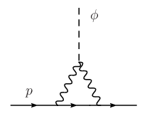
The Yukawa coupling (8.2) leads to non-newtonian forces between two test masses and , due to exchange. The total potential between 1 and 2 is
| (8.4) |
Here is the total number of protons in the test body . In (8.4) we have neglected the new electron-proton and electron-electron force since the corresponding value for in the case of the electron is smaller than (8.3) by a factor . When the two test bodies are constituted each by only one element, with atomic numbers and , and mass numbers and , we can approximate (8.4) by
| (8.5) |
where now in the second term inside the square brackets i.e., the term containing the correction to the newtonian potential, we have approximated .
The non-newtonian part of the potential we have obtained has two clear properties: it has a finite range and depends on the composition of the bodies, i.e. on their values. We can use the abundant experimental bounds on fifth-type forces to limit our parameter as a function of .
To see how we proceed we find now the limit in the interesting ranges mm, with the PVLAS results in mind. Bounds on new forces have been obtained by experiments designed to measure very small forces. In the submillimeter range, in 1997 authors of ref. [159] using a micromechanical resonator designed to measure Casimir force between parallel plates gave limits on new forces, and they also estimated the corresponding limits on the mass and inverse coupling constant of scalar particles. Also, strong experimental limits on new forces have been published in [160], where they use a torsion pendulum and a rotating attractor in the framework of tests of the gravitational inverse-square law. The most strict bounds have been obtained very recently by using torsion-balance experiments [161, 162].
The limit from the experiment presented in ref. [161, 162] for eV is
| (8.6) |
which leads, introducing the conservative values for of 0.4,
| (8.7) |
To obtain now a limit on , we will simply put the value of the log in (8.3) equal to 1; this will lead to a conservative limit since . With this, we obtain
| (8.8) |
Such a high lower bound implies that no signal of a particle of mass meV should be seen in experiments like PVLAS [43, 158] or CAST [79]. In order to reach our conclusion we have to assume that the lagrangian (8.1) is valid up to high energy scales .

We can proceed in analogous way and find bounds for other values of . They are shown in Fig. 2, and as we see, the limits on are very tight.
Our final discussion is about modified vertices. Examples of such models have been developed in [1, 2] with the motivation of making compatible the PVLAS particle interpretation with the bounds coming from stellar energy loss and a fortiori with the CAST results. In these models the ALP does couple to new paraphotons and has not a direct coupling to photons. The vertex arises because there is kinetic photon-paraphoton mixing. Also, a paraphoton mass induces an effective photon form factor such that the coupling is reduced for .
When there is a form factor with a low scale , the analysis shown in this paper should be modified accordingly. In such a case the lagrangian in (8.1) is valid only for photons with momentum such that . The induced Yukawa will be suppressed with respect to the value (8.3), and thus the lower bound (8.8) can be very much relaxed if indeed is a low energy scale.
In order to quantify our last assertion, we have calculated the induced Yukawa coupling when the photons have a modified propagator
| (8.9) |
Now the diagram of Fig.1 is finite. The calculation of the coupling to protons , at leading order in gives
| (8.10) |
To find the potential between bodies we have to take into account the coupling to protons as well as to electrons, because (8.10) is independent of the mass of the fermion. The potential when having a form factor (8.9) is given by
| (8.11) |
We see that the new non-standard potential (8.11) has a Yukawa coupling that compared to (8.3) is suppressed by a factor of order . The parameter introduced in [1, 2] is not fully specified by the theory. In order to solve the PVLAS-CAST puzzle and if we do not wish too different scales in the model, should be in the subeV range with a preferred value meV. For this value, the bound (8.8) would relax by 12 orders of magnitude, bringing it close to the PVLAS value GeV. Remarkably enough, experiments searching for new forces and testing Casimir forces at the submm lengths may be sensitive to the potential (8.11) that corresponds to a vertex with the form factor (8.9).
Note added : The fact that a scalar-photon-photon coupling gives rise to new forces and leads to a bound on has been independently realized by Shmuel Nussinov [173].
Chapter 9 Final Discussion and Conclusions
The PVLAS signal has attracted a lot of theoretical work since the publication of their signal. As a consequence, many arguments have arose that are relevant for my work. On the other hand it is mandatory to include some comments on the actual status of the field together with future prospects. In next section I address both tasks. Finally I present a short summary and my conclusions.
9.1 Final discussion
The original work of this thesis starts in Chapter 5, corresponding to reference [1]. In this paper we quantified the inconsistency between the PVLAS ALP interpretation and the astrophysical bounds (HB lifetime and Helioscope experiments) and studied two mechanisms for avoiding these bounds. Both of them require the existence of new particles together with the PVLAS ALP. The energy scale related to this new physics is closer to the suggested ALP mass meV than to the inverse coupling GeV. This can be achieved considering that the ALP coupling to two photons proceeds through photon-paraphoton mixing and a mediator MCP which couples the paraphoton field with the ALP.
The first mechanism consists in providing a strong interaction of ALPs with the stellar medium in such a way that ALPs produced in stellar media can be reabsorbed inside the stellar plasma. The second proposes that the Primakoff production of ALPs at the relatively high temperatures of stellar interiors is suppressed with respect to the PVLAS experiment, performed in vacuum. Although these general mechanisms remain to be valid, (and have probably inspired other works trying to solve the PVLAS-astrophysics puzzle) the concrete models we presented are not reliable anymore. The trapping mechanism has to pay the price of introducing a new relatively strong interaction between low mass novel particles and photons. In the same article [1] we see that a background of paraphotons and ALPs will be formed in the early universe and this would contradict the actual observations of the cosmic microwave background, pointing to a transparent universe at temperatures around eV.
Nevertheless, we decided to include this model for two reasons.First, because it allowed us to introduce paraphoton models as our theoretical tool to interpret the PVLAS signal as a smoking gun of low energy physics and second because it illustrates one of the known mechanisms to avoid the astrophysical bounds, so it might be inspiring for further investigations along that line. Indeed, the trapping mechanism has originated at least a couple of works trying to evade the stellar bounds on ALPs [71, 72] and paraphoton models have been further used for model building around the PVLAS signal.
The second mechanism has proven to be more fruitful because it does not require a new strong interaction, but contrarily, it suggests that the new physics can come into the game to suppress the Primakoff production in stars, i.e. to make the ALP-photon interactions feebler. The concrete model presented uses a new confining force, in the spirit of QCD, that makes the ALP a composite particle of millicharged preons, providing a production form factor that suppresses the stellar emission. This models has nowadays become obsolete. The reason is that, in this case, the main production channel of ALPs in stars would not be the Primakoff production but the plasmon decay into a pair of preons that would further hadronize into many ALPs and other preonic bound states11 1 I acknowledge interesting conversations at this respect with Joerg Jaeckel, Andreas Ringwald, Alex Pomarol, Georg Raffelt.. Although the final products of the decay will be very different, such a process occurs at the same rate than the plasmon decay into a pair of MCPs I used in Chapter 3 so that the stellar energy loss bounds apply also in this case.
In our second paper [2], presented in Chapter 6, we recovered the idea of the suppression of stellar ALP production within the framework of paraphoton models to provide a new model. There, the coupling between the MCP and photons proceeds through two possible intermediate states, two paraphotons, in such a way that they interfere negatively canceling the amplitude of any physical process when the square of the momentum carried by the paraphotons tends to infinity. The suppression of the stellar production achieved with this model can be very strong but has the disadvantage that the cancelation between the contributions from the two paraphotons has to be carefully tuned. Beyond this prejudice, the model is able not only to reconcile the PVLAS ALP with astrophysics (HB lifetime and Helioscopes) but also with 5th force searches if the PVLAS ALP turns out to be finally a particle [4].
At the moment of writing this paper we were already aware of the above criticism to the suppression model presented in [1] so this model focused on suppressing the plasmon decay into MCP pairs and not the Primakoff production.
An alternative interpretation of the PVLAS signal can be made in terms of the pair production of millicharged particles (MCPs) with mass eV and charge [27]. Basically this means that our model [2] is a candidate for explaining the PVLAS signal even in the absence of an ALP. Of course, the MCP-PVLAS interpretation based on [2] is more economical than the one originally presented in [2] because it requires one particle less.
In order to know if the ALP is superfluous or not we will have to wait until more experimental data is available. The PVLAS experiment is sensitive to the parity of the ALP or the bosonic/fermionic character of the MCP. Also, a positive signal in a light-shining-through-walls (LSW) experiment could be the smoking gun of the existence of the ALP, since MCPs can not contribute to it. The program of discriminating between these two possibilities has been started in [47], and I say has been started because an exact study of the PVLAS signal in our model [2] has not yet been performed after we know that just MCP production can do the job. A combined analysis of coherent ALP production and MCP production is in current development. Yet a new source of rotation has been recently discovered, the coherent production of paraphotons in magnetic fields in models with light paracharged particles [92]. This adds up a new difficulty to this combined analysis because now the model [2] without an ALP will give a positive signal in future LSW experiments.
Remarkably, the advent of the MCP interpretation has motivated some works proposing new bounds for the existence of MCPs [88, 108, 85]. In the last reference, the impact of MCPs in the CMB radiation is studied and it is nowadays the most firm constraint for the model [2]. Some work is in progress to ensure if the bounds presented are really model independent or if they can be circumvented in any region of the parameter space or by means of soft modifications of the model [2]. Notably, the CMB constraints do not rule out the bare ALP interpretation.
Going back to the features of the model [2] one might feel uncomfortable not only with so many parameters and fields introduced but also with the apparently arbitrary choice of charge assignments. At this respect it is interesting to note that our model has been justified from string theory [143], were the existence of additional symmetries is generally predicted as well as particles in the required representations.
In [3] I present a general study of the suppression scenario suggested in [1]. We parameterize a general suppression mechanism allowing the ALP mass and coupling constant to depend on any environmental physical quantity that can make a difference between the clean PVLAS setup and the hot and dense stellar plasmas. Because in the suppression scenario the Helioscope bounds are more robust than the energy loss bounds we focus exclusively on the case of the Sun.
In the models worked out in [1, 2] we performed a rough estimate of the stellar lifetime bounds in the presence of suppression of the ALP production: we computed the whole ALP emission from the values of the relevant parameters at the stellar center. This is indeed a quite good approximation in the absence of suppression but it is dangerous within our suppression models for the following reason: our models are designed to be more effective in suppressing ALP production wherever the conditions of the production are more extreme. For instance, in [1] the suppression of the Primakoff production depends on the screening scale, , which is maximum in the stellar center because the density of screening charges is much higher there than in outer shells. Therefore, the suppression computed is overestimated in the external layers of the stars. In order to provide better estimates we computed more accurate bounds by integrating the ALP emission over the most recent solar model available.
In [3] I differentiate two possibilities for a general suppression scenario: (a) The sensitive parameter is an average environmental parameter like temperature or matter density that, given a solar model, depends only on the position of the Sun and (b) the parameter is the momentum transfer of the Primakoff conversion. Our conclusions are very interesting, in the first case the conciliation of PVLAS and CAST demands that the suppression of the Primakoff ALP production is complete in almost the whole volume of the Sun (up to a of the solar radius). In the second, the scale at which the photon propagator must be cut-off is eV. It is interesting to note that this is the scale suggested in our model [1] by means of a much simpler estimation.
While at the time of publication of [1] our model was the unique solution for the PVLAS-astrophysics puzzle some alternatives begun to show up soon after. Interestingly enough, at least two of them fit exactly our scheme of suppression driven by an environmental parameter in [3]. Thus our paper can be used to further constrain these new proposals.
In [116] the authors propose an intricate mechanism for getting a ALP coupling that vanishes abruptly at a temperature between PVLAS and the stars due to the phase transition of another scalar field. This model fits exactly our model independent scheme [3]. Our study clearly predicts that the value of the critical temperature must be below eV (See table 7.2) in order to satisfy the CAST bounds because the ALP emission must be suppressed not only at keV but essentially at every place of the whole Sun.
Other model has recently appear in [174]. There the authors propose that the PVLAS ALP can be of the chameleon type [117], an exotic field whose mass depends on the environmental matter density, . This possibility had been indeed briefly examined in [3]. If the mass of the chameleon increases so much under the solar conditions such that its production is kinetically impossible then we have the suppression required to evade the CAST bounds. In this case the conclusions of our paper are much more dramatic than in the previous case. The authors use a typical matter density in the Sun gcm-3 while we find that the suppression should be fully active above gcm-3.
All the models presented in this thesis show that reconciling the PVLAS ALP with astrophysics (in particular with the Helioscope measurements) does require new physics at accessible scales. As I pointed out in Chapter 4 the ALP physics must dramatically change in between the PVLAS and stellar environments. Notably, this suggests that the PVLAS particle (ALP or MCP) is not likely to exist alone and thus the new generation of low energy experiments can eventually discover several particles.
A program to discriminate between the different possibilities is currently under way. As the conditions in the solar plasma are not so extreme, they can be testable in laboratories and therefore new experimental efforts are crucial to test the PVLAS particle interpretation.
Interestingly enough, many experiments have been recently proposed to test the PVLAS signal. At least three of them have currently began to work. The BMV and Q collaborations are building PVLAS-type experiments looking for vacuum dichroism and birefringence while the ALPS collaboration is currently building a LSW experiment. The same PVLAS collaboration will soon perform a LSW run after a soft modification of their setup. Other LSW experiments have been proposed at Jefferson Lab and CERN, the LIPPS and OSQAR collaborations. A detailed review of the status of the experimental tests of the PVLAS signal can be found in [175].
Finally it is worth mentioning that the PVLAS collaboration has been releasing new data in several conferences during the last years. Together with the published measurements of the rotation of the polarization plane of a eV laser (red) they have presented rotation data for a smaller wavelength light ( eV, green) and ellipticity measurements with both lasers. The absolute values of rotation and ellipticity data agree with an ALP interpretation but it is not the case when one takes into account the measured signs. Ellipticity data favors an ALP while rotation data with the green laser favors a ALP. If these results are confirmed then the bare ALP interpretation would be ruled out. It remains to be investigated if the model in [2] could accommodate this results when the effects of MCP and paraphoton production are taken into account.
The fact that PVLAS ellipticy measurements point to a ALP motivated us to consider the bounds presented in [4]. As already noted, these bounds are the strongest constraints for a ALP interpretation. However, they were unknown at the time of publishing [2] and [3] and therefore the requirements we derive there for a ALP to satisfy the HB lifetime and Helioscope bounds are not sufficient to ensure a PVLAS ALP interpretation. As a remarkable fact, the model [2] turned out to evade the force bounds and chameleon models as [174] are in principle able to satisfy them as well.
9.2 Conclusions
In this thesis I have been concerned with some of the problems that arise when trying to interpret the measurements of the PVLAS collaboration [43] in terms of a novel, low mass, spin-zero particle coupled to light [33] we call ALP.
My main concern has been to investigate whether the strong astrophysical bounds, excluding such a particle, could be circumvented in any particle physics model. I have discussed two mechanisms, trapping the new particles in the stars and suppressing their production in stellar environments with respect to the PVLAS experiment. The second has given more reliable results.
In order to build models that either trap or suppress the number of stellar ALPs I have invoked new particles, namely paraphotons and millicharged particles.
Notably the scale of the masses required for these new particles is very low eV, a very suggestive value. I have also made a model-independent study of general suppression mechanisms. This work also points to new phenomena accessible in earth-ground laboratory experiments. Therefore, new laboratory experiments have been encouraged.
In the near future, many experiments testing the PVLAS signal will be performed and this thesis suggests that the PVLAS particle could not be alone. Therefore, having different kinds of experiments will be crucial for confronting different models.
Recently, new strong constraints on the PVLAS ALP as well as on paraphotons and millicharged particles have been derived. I have shown that force searches set strong limits on the PVLAS particle if it is a . On the other hand, the CMB has been proven to be sensitive to the existence of millicharged particles. Notably, my best model is able to avoid both constraints.
If the PVLAS signal is confirmed and firmly established, I believe that few particle physics models could solve the strong conflict with astrophysics. In these thesis I have developed solutions that involve physics at very low energies.
Appendix A Schizons
If we let our ALP to couple to light through both interactions in (2.4) parity is not conserved by the ALP interactions. Therefore, the ALP has not definite parity and because of that it can be called a “schizon” [176]. In this case, we find a complicated mixing problem
| (A.1) |
Where in the relativistic limit for photons traveling along the -direction. In absence of Cotton-Mouton and faraday effects (vacuum) the problem simplifies notably. By means of a rotation of angle in the space it can be decoupled into
| (A.2) |
where are the photon states coupling to the schizon and neutral respectively, and is the effective coupling constant. We have found exactly equation (2.20) with the following replacements , so equations (2.33),(2.34) are also solutions for the schizon case. In order to give a result for the induced rotation and ellipticity in PVLAS we have to rotate back to . In the weak mixing regime, I get
| (A.3) | |||||
| (A.4) |
The schizon couplings add at least two new ingredients to the ALP interpretation. First, they provide a phase shift between the photon initial polarization and the final rotation. By sending to zero we recover the two pure parity cases, because in this cases , namely and . The rotations shown again to be of opposite sign. Secondly, the photon state coupling to depends on the direction of propagation ( depends on the sign , namely )
| (A.5) | |||||
| (A.6) |
As a consequence the effect of multiple reflections inside a Fabry-Perot cavity can be considerably diminished [177], a fact that worsens the PVLAS discrepancy with astrophysics. This can be easily seen from (A.3) and (A.4) since the sum of the two rotations(ellipticities) acquired after two consecutive passes in opposite directions is
| (A.7) |
which is maximum for , namely, the pure parity cases. A similar expression holds for the ellipticity. A remarkably fact in this case is that the information of and cannot be extracted separately and thus PVLAS is not able to discriminate is the ALP is an schizon or not.
Bibliography
- [1] E. Masso and J. Redondo, JCAP 0509 (2005) 015 [arXiv:hep-ph/0504202].
- [2] E. Masso and J. Redondo, Phys. Rev. Lett. 97, 151802 (2006), hep-ph/0606163.
- [3] J. Jaeckel, E. Masso, J. Redondo, A. Ringwald, and F. Takahashi, Phys. Rev. D75, 013004 (2007), hep-ph/0610203.
- [4] A. Dupays, E. Masso, J. Redondo, and C. Rizzo, Phys. Rev. Lett. 98, 131802 (2007), hep-ph/0610286.
- [5] E. C. G. Stueckelberg, Phys. Rev. 52, 41 (1937).
- [6] E. C. G. Stueckelberg, Helv. Phys. Acta 11, 225 (1938).
- [7] E. C. G. Stueckelberg, Helv. Phys. Acta 11, 299 (1938).
- [8] E. C. G. Stueckelberg, Helv. Phys. Acta 11, 312 (1938).
- [9] S. Weinberg, Phys. Rev. D11, 3583 (1975).
- [10] G. ’t Hooft, Phys. Rept. 142, 357 (1986).
- [11] K. Fujikawa, Phys. Rev. Lett. 42, 1195 (1979).
- [12] S. Weinberg, The quantum theory of fields. Vol. 2: Modern applications , Cambridge, UK: Univ. Pr. (1996) 489 p.
- [13] R. D. Peccei, Lect. Notes Phys. 741 (2008) 3 [arXiv:hep-ph/0607268].
- [14] V. Baluni, Phys. Rev. D19, 2227 (1979).
- [15] R. D. Peccei and H. R. Quinn, Phys. Rev. Lett. 38, 1440 (1977).
- [16] R. D. Peccei and H. R. Quinn, Phys. Rev. D16, 1791 (1977).
- [17] S. Weinberg, Phys. Rev. Lett. 40, 223 (1978).
- [18] F. Wilczek, Phys. Rev. Lett. 40, 279 (1978).
- [19] M. Dine, W. Fischler, and M. Srednicki, Phys. Lett. B104, 199 (1981).
- [20] J. E. Kim, Phys. Rev. Lett. 43, 103 (1979).
- [21] D. B. Kaplan, Nucl. Phys. B260, 215 (1985).
- [22] Y. Chikashige, R. N. Mohapatra, and R. D. Peccei, Phys. Rev. Lett. 45, 1926 (1980).
- [23] Y. Chikashige, R. N. Mohapatra, and R. D. Peccei, Phys. Lett. B98, 265 (1981).
- [24] F. Wilczek, Phys. Rev. Lett. 49, 1549 (1982).
- [25] C. Vafa and E. Witten, Phys. Rev. Lett. 53, 535 (1984).
- [26] L. B. Okun, Sov. Phys. JETP 56, 502 (1982).
- [27] H. Gies, J. Jaeckel, and A. Ringwald, Phys. Rev. Lett. 97, 140402 (2006), hep-ph/0607118.
- [28] B. Holdom, Phys. Lett. B259, 329 (1991).
- [29] K. R. Dienes, C. F. Kolda, and J. March-Russell, Nucl. Phys. B492, 104 (1997), hep-ph/9610479.
- [30] E. Masso and J. Redondo, AIP Conf. Proc. 878, 387 (2006) [arXiv:hep-ph/0609275].
- [31] J. Redondo, (2006), hep-ph/0610213.
- [32] H. Primakoff, Phys. Rev. 81, 899 (1951).
- [33] L. Maiani, R. Petronzio, and E. Zavattini, Phys. Lett. B175, 359 (1986).
- [34] S. L. Adler, Annals Phys. 67, 599 (1971).
- [35] T. Erber, Nature 190, 25 (1961).
- [36] E. Iacopini and E. Zavattini, Phys. Lett. B85, 151 (1979).
- [37] G. G. Raffelt and G. D. Starkman, Phys. Rev. D40, 942 (1989).
- [38] A. A. Anselm and N. G. Uraltsev, Phys. Lett. B114, 39 (1982).
- [39] Y. Semertzidis et al., Phys. Rev. Lett. 64, 2988 (1990).
- [40] R. Cameron et al., Phys. Rev. D47, 3707 (1993).
- [41] D. Bakalov et al., Nucl. Phys. B (Proc. Suppl.) 35, 180 (1994).
- [42] M. Born and E. Wolf, Principles of Optics (Pergamon Press, 1980), 691-692.
- [43] PVLAS, E. Zavattini et al., Phys. Rev. Lett. 96, 110406 (2006), hep-ex/0507107.
- [44] G. Cantatore, (2006), Talk given at the Conference: Axions in the Institute for advanced study, http://www.sns.ias.edu/ axions/talks/GiovanniCantatore.pdf.
- [45] PVLAS collaboration, G. Cantatore, (2006), Talk given at the 2nd ILIAS-CERN-CAST Axion Academic Training, http://cast.mppmu.mpg.de/.
- [46]
U. Gastaldi,
PVLAS results on rotation of polarized light in a high magnetic
field,
Talk given at the Conference “QCD06”,
http://www.lpta.univ-montp2.fr/users/qcd/prog06.html, 2006. - [47] M. Ahlers, H. Gies, J. Jaeckel, and A. Ringwald, Phys. Rev. D75, 035011 (2007), hep-ph/0612098.
- [48] S. Das, P. Jain, J. P. Ralston, and R. Saha, JCAP 0506, 002 (2005), hep-ph/0408198.
- [49] E. Gabrielli, K. Huitu, and S. Roy, Phys. Rev. D74, 073002 (2006), hep-ph/0604143.
- [50] G. Raffelt and L. Stodolsky, Phys. Rev. D37, 1237 (1988).
- [51] J. T. Mendonca, J. Dias de Deus and P. Castelo Ferreira, Phys. Rev. Lett. 97, 100403 (2006) [Erratum-ibid. 97, 269901 (2006)] [arXiv:hep-ph/0606099].
- [52] S. L. Adler, (2006), hep-ph/0611267.
- [53] C. Biggio, E. Masso, and J. Redondo, (2006), hep-ph/0604062.
- [54] J. Jaeckel, E. Masso, J. Redondo, A. Ringwald, and F. Takahashi, (2006), hep-ph/0605313.
- [55] A. C. Melissinos, (2007), hep-ph/0702135.
- [56]
PVLAS collaboration, U. Gastaldi,
Talk at ICHEP‘06, Moscow,
http://ichep06.jinr.ru/reports/42_1s2_13p10_gastaldi.ppt. - [57] S.-J. Chen, H.-H. Mei, W.-T. Ni, and J.-S. Wu, (2003), hep-ex/0308071.
- [58] G. Zavattini, PVLAS, Talk given at the XII International Workshop on Neutrino Telescopes, Venice, 2007.
- [59] G. G. Raffelt, (2005), hep-ph/0504152.
- [60] G. G. Raffelt, (2006), hep-ph/0611118.
- [61] E. Masso and R. Toldra, Phys. Rev. D52, 1755 (1995), hep-ph/9503293.
- [62] E. Masso and R. Toldra, Phys. Rev. D55, 7967 (1997), hep-ph/9702275.
- [63] V. Popov, Turkish Journal of Physics 23, 943 (1999).
- [64] P. K. Durrel and W. E. Harris, Astronomical Journal 105, 1420 (1993).
- [65] G. G. Raffelt, Chicago, USA: Univ. Pr. (1996) 664 p.
- [66] E. Braaten and D. Segel, Phys. Rev. D48, 1478 (1993), hep-ph/9302213.
- [67] D. A. Dicus, E. W. Kolb, V. L. Teplitz, and R. V. Wagoner, Phys. Rev. D18, 1829 (1978).
- [68] J. A. Grifols and E. Masso, Phys. Lett. B173, 237 (1986).
- [69] J. A. Grifols, E. Masso, and S. Peris, Mod. Phys. Lett. A4, 311 (1989).
- [70] J. A. Grifols, E. Masso, and S. Peris, Phys. Lett. B220, 591 (1989).
- [71] P. Jain and S. Mandal, (2005), astro-ph/0512155.
- [72] R. Foot and A. Kobakhidze, (2007), hep-ph/0702125.
- [73] J. N. Bahcall and R. K. Ulrich, Rev. Mod. Phys. 60, 297 (1988).
- [74] Particle Data Group, W. M. Yao et al., J. Phys. G33, 1 (2006).
- [75] P. Sikivie, Phys. Rev. Lett. 51, 1415 (1983), [Erratum-ibid. 52, 695 (1984)].
- [76] K. van Bibber, P. M. McIntyre, D. E. Morris, and G. G. Raffelt, Phys. Rev. D39, 2089 (1989).
- [77] S. Moriyama et al., Phys. Lett. B434, 147 (1998), hep-ex/9805026.
- [78] D. M. Lazarus, G. C. Smith, R. Cameron, A. C. Melissinos, G. Ruoso, Y. K. Semertzidis and F. A. Nezrick, Phys. Rev. Lett. 69, 2333 (1992).
- [79] CAST collaboration, K. Zioutas et al., Phys. Rev. Lett. 94, 121301 (2005), hep-ex/0411033.
- [80] S. Davidson, S. Hannestad, and G. Raffelt, JHEP 05, 003 (2000), hep-ph/0001179.
- [81] R. H. Cyburt, B. D. Fields, K. A. Olive and E. Skillman, Astropart. Phys. 23, 313 (2005) [arXiv:astro-ph/0408033].
- [82] M. I. Dobroliubov and A. Y. Ignatiev, Phys. Rev. Lett. 65, 679 (1990).
- [83] S. Davidson, B. Campbell, and D. C. Bailey, Phys. Rev. D43, 2314 (1991).
- [84] T. P. Walker, G. Steigman, D. N. Schramm, K. A. Olive, and B. Fields, Astrophys. J. 413, 562 (1993).
- [85] A. Melchiorri, A. Polosa, and A. Strumia, (2007), hep-ph/0703144.
- [86] M. Kleban and R. Rabadan, (2005), hep-ph/0510183.
- [87] S. N. Gninenko, N. V. Krasnikov, and A. Rubbia, (2006), hep-ph/0612203.
- [88] H. Gies, J. Jaeckel, and A. Ringwald, Europhys. Lett. 76, 794 (2006), hep-ph/0608238.
- [89] L. Lilje et al., Nucl. Instrum. Meth. A524, 1 (2004), physics/0401141.
- [90] A. A. Anselm, N. G. Uraltsev, and M. Y. Khlopov, Sov. J. Nucl. Phys. 41, 1060 (1985).
- [91] K. Van Bibber, N. R. Dagdeviren, S. E. Koonin, A. Kerman, and H. N. Nelson, Phys. Rev. Lett. 59, 759 (1987).
- [92] M. Ahlers, H. Gies, J. Jaeckel, J. Redondo and A. Ringwald, Phys. Rev. D 76 (2007) 115005 [arXiv:0706.2836 [hep-ph]].
- [93] E. Gabrielli and M. Giovannini, (2007), hep-ph/0702197.
- [94] E. Lundstrom et al., Phys. Rev. Lett. 96, 083602 (2006), hep-ph/0510076.
- [95] T. Heinzl et al., Opt. Commun. 267, 318 (2006), hep-ph/0601076.
- [96] P. Sikivie, D. B. Tanner, and K. van Bibber, (2007), hep-ph/0701198.
- [97] C. A. Baker et al., Phys. Rev. Lett. 97, 131801 (2006), hep-ex/0602020.
- [98] C. N. Yang, Phys. Rev. 77, 242 (1950).
- [99] L. D. Landau, Dokl. Akad. Nauk SSSR 60, 207 (1948).
- [100] S. Asai, S. Orito, K. Yoshimura, and T. Haga, Phys. Rev. Lett. 66, 2440 (1991).
- [101] A. Czarnecki, Acta Phys. Polon. B30, 3837 (1999), hep-ph/9911455.
- [102] T. Mitsui et al., Phys. Rev. Lett. 70, 2265 (1993).
- [103] A. Badertscher et al., Phys. Rev. D75, 032004 (2007), hep-ex/0609059.
- [104] M. Knecht and A. Nyffeler, Phys. Rev. D65, 073034 (2002), hep-ph/0111058.
- [105] B. E. Lautrup and E. De Rafael, Phys. Rev. 174, 1835 (1968).
- [106] P. J. Mohr and B. N. Taylor, Rev. Mod. Phys. 72, 351 (2000).
- [107] S. Bourzeix et al., Phys. Rev. Lett. 76, 384 (1996).
- [108] M. Gluck, S. Rakshit, and E. Reya, (2007), hep-ph/0703140.
- [109] S. R. Lundeen and F. M. Pipkin, Phys. Rev. Lett. 46, 232 (1981).
- [110] E. W. Hagley and F. M. Pipkin, Phys. Rev. Lett. 72, 1172 (1994).
- [111] S. G. Karshenboim, Physics Reports 422, 1 (2005).
- [112] G. B. Gelmini, S. Nussinov, and T. Yanagida, Nucl. Phys. B219, 31 (1983).
- [113] F. Ferrer and J. A. Grifols, Phys. Rev. D58, 096006 (1998), hep-ph/9805477.
- [114] J. A. Grifols, E. Masso and R. Toldra, Phys. Lett. B 389, 563 (1996) [arXiv:hep-ph/9606377].
- [115] D. F. Bartlett and S. Loegl, Phys. Rev. Lett. 61, 2285 (1988).
- [116] R. N. Mohapatra and S. Nasri, (2006), hep-ph/0610068.
- [117] J. Khoury and A. Weltman, Phys. Rev. Lett. 93, 171104 (2004), astro-ph/0309300.
- [118] G. G. Raffelt, Ann. Rev. Nucl. Part. Sci. 49, 163 (1999), hep-ph/9903472.
- [119] R. J. Creswick et al., Phys. Lett. B427, 235 (1998), hep-ph/9708210.
- [120] Y. Inoue et al., Phys. Lett. B536, 18 (2002), astro-ph/0204388.
- [121] E. D. Carlson and P. Salati, Phys. Lett. B218, 79 (1989).
- [122] H. Georgi, P. H. Ginsparg, and S. L. Glashow, Nature 306, 765 (1983).
- [123] B. Holdom, Phys. Lett. B178, 65 (1986).
- [124] B. Holdom, Phys. Lett. B166, 196 (1986).
- [125] R. Foot, A. Y. Ignatiev, and R. R. Volkas, Phys. Lett. B503, 355 (2001), astro-ph/0011156.
- [126] B. A. Dobrescu, Phys. Rev. Lett. 94, 151802 (2005), hep-ph/0411004.
- [127] R. I. Dzhelyadin et al., Phys. Lett. B94, 548 (1980).
- [128] TPC/Two Gamma, H. Aihara et al., Phys. Rev. Lett. 64, 172 (1990).
- [129] CELLO, H. J. Behrend et al., Z. Phys. C49, 401 (1991).
- [130] CLEO, J. Gronberg et al., Phys. Rev. D57, 33 (1998), hep-ex/9707031.
- [131] A. Bramon and E. Masso, Phys. Lett. B104, 311 (1981).
- [132] L. Ametller, L. Bergstrom, A. Bramon, and E. Masso, Nucl. Phys. B228, 301 (1983).
- [133] G. P. Lepage and S. J. Brodsky, Phys. Rev. D22, 2157 (1980).
- [134] L. Ametller, J. Bijnens, A. Bramon, and F. Cornet, Phys. Rev. D45, 986 (1992).
- [135] A. Z. Dubnickova, S. Dubnicka, G. Pancheri, and R. Pekarik, Nucl. Phys. Proc. Suppl. 126, 71 (2004), hep-ph/0401007.
- [136] J. P. B. C. de Melo, T. Frederico, E. Pace, and G. Salme, Phys. Lett. B581, 75 (2004), hep-ph/0311369.
- [137] B.-W. Xiao and B.-Q. Ma, Phys. Rev. D71, 014034 (2005), hep-ph/0501160.
- [138] G. G. Raffelt, Phys. Rev. D33, 897 (1986).
- [139] A. Ringwald, Phys. Lett. B569, 51 (2003), hep-ph/0306106.
- [140] S. Lamoreaux, Nature 441N7089, 31 (2006).
- [141] A. Ringwald, http//www.desy.de/ringwald/axions/talks/patras.pdf.
- [142] E. R. Williams, J. E. Faller, and H. A. Hill, Phys. Rev. Lett. 26, 721 (1971).
- [143] S. A. Abel, J. Jaeckel, V. V. Khoze and A. Ringwald, arXiv:hep-ph/0608248.
- [144] A. Ringwald, J. Phys. Conf. Ser. 39, 197 (2006), hep-ph/0511184.
- [145] I. Antoniadis, A. Boyarsky and O. Ruchayskiy, arXiv:hep-ph/0606306.
- [146] R. Rabadan, A. Ringwald, and K. Sigurdson, Phys. Rev. Lett. 96, 110407 (2006), hep-ph/0511103.
- [147] P. Pugnat, M. Kral, A. Siemko, L. Duvillaret, M. Finger and J. Zicha, Czech. J. Phys. 55, A389 (2005).
- [148] U. Gastaldi, arXiv:hep-ex/0605072.
- [149] A. V. Afanasev, O. K. Baker and K. W. McFarlane, arXiv:hep-ph/0605250.
- [150] U. Kotz, A. Ringwald, and T. Tschentscher, (2006), hep-ex/0606058.
- [151] BMV collaboration, C. Rizzo, (2006), Talk given at the 2nd ILIAS-CERN-CAST Axion Academic Training, http://cast.mppmu.mpg.de/.
- [152] J. A. Frieman, S. Dimopoulos, and M. S. Turner, Phys. Rev. D36, 2201 (1987).
- [153] G. G. Raffelt and D. S. P. Dearborn, Phys. Rev. D36, 2211 (1987).
- [154] J. N. Bahcall, A. M. Serenelli, and S. Basu, Astrophys. J. 621, L85 (2005), astro-ph/0412440.
- [155] J. N. Bahcall and M. H. Pinsonneault, Rev. Mod. Phys. 67, 781 (1995), hep-ph/9505425.
- [156] J. N. Bahcall, W. F. Huebner, S. H. Lubow, P. D. Parker, and R. K. Ulrich, Rev. Mod. Phys. 54, 767 (1982).
- [157] S. J. Asztalos et al., Phys. Rev. D69, 011101 (2004), arXiv:astro-ph/0310042.
- [158]
See the talks of G. Cantatore and G. Ruoso at IDM 06,
http://elea.inp.demokritos.gr/idm2006files/talks/, 2006. - [159] G. Carugno, Z. Fontana, R. Onofrio, and C. Rizzo, Phys. Rev. D55, 6591 (1997).
- [160] C. D. Hoyle et al., Phys. Rev. D70, 042004 (2004), hep-ph/0405262.
- [161] D. J. Kapner et al., Phys. Rev. Lett. 98, 021101 (2007), hep-ph/0611184.
- [162] E. G. Adelberger et al., (2006), hep-ph/0611223.
- [163] J. O. Dickey et al., Science 265, 482 (1994).
- [164] J. G. Williams et al., Phys. Rev. D53, 6730 (1996).
- [165] R. Onofrio, New Journal of Physics 8, 237 (2006).
- [166] Y. Su et al., Phys. Rev. D50, 3614 (1994).
- [167] J. K. Hoskins et al., Phys. Rev. D32, 3084 (1985).
- [168] J. K. Hoskins et al., Phys. Rev. Lett. 44, 1645 (1980).
- [169] J. S. Smullin et al., Phys. Rev. D72, 122001 (2005), arXiv:hep-ph/0508204.
- [170] J. Chiaverini et al., Phys. Rev. Lett. 90, 15101 (2003), arXiv:hep-ph/0209325.
- [171] S. K. Lamoreaux, Phys. Rev. Lett. 78, 5 (1997).
- [172] S. K. Lamoreaux, Phys. Rev. Lett. 81, 5475 (1998).
- [173] S. Nussinov, private communication.
- [174] P. Brax, C. van de Bruck and A. C. Davis, Phys. Rev. Lett. 99, 121103 (2007) [arXiv:hep-ph/0703243].
- [175] A. Ringwald, (2007), arXiv:0704.3195 [hep-ph].
- [176] C. T. Hill and G. G. Ross, Nucl. Phys. B311, 253 (1988).
- [177] Y. Liao, (2007), arXiv:0704.1961 [hep-ph].