Quantum Particle Production
at Sudden Singularities

In ref. [1] it was shown that classical general relativistic Friedmann universes allow finite-time singularities to occur in which the scale factor, $a(t)$, its time derivative, $\dot{a}$, and the density, $\rho,$ remain finite whilst a singularity occurs in the fluid pressure, $p\rightarrow+\infty,$ and the expansion acceleration, $\ddot{a}\rightarrow\infty$. Remarkably, the strong energy condition continues to hold, $\rho+3p>0.$ Analogous solutions are possible in which the singularity can occur only in arbitrarily high derivatives of $a(t),$[2]. This behaviour occurs independently of the 3-curvature of the universe and can prevent closed Friedmann universes that obey the strong energy condition from recollapsing [3]. Subsequently, a number of studies have been carried out which generalise these results to different cosmologies and theories of gravity [4], classify the other types of future singularity that can arise during the expansion of the universe [5], and explore some observational constraints on their possible future occurrence in our Universe [6].

In this paper we extend these studies to consider some quantum implications of a sudden singularity. Specifically, we want to know if quantum particle production can dominate over the classical background density on approach to a sudden singularity and stop it occurring or modify its properties, as can be the case for the Big Rip future singularities [7, 8]. The results of such a study are also of interest for observational probes of finite-time singularities. In an inhomogeneous universe it would be possible for us in principle to observe a sudden singularity on our past light cone. What might we see? If quantum effects produce profuse particle production then there might be observable effects from local sudden singularities. In this respect, sudden singularities are also of interest with regard to proposed measures of gravitational entropy associated with invariants of the Weyl curvature [9]. The Weyl invariant will not diverge on approach to a sudden singularity (and there is no geodesic incompleteness [10]) and so it may represent a part of a soft future boundary of the universe with low gravitational entropy – which could be as close as 8.7 Myr to the future [6]. The effects of loop quantum gravity have been studied in cosmologies exhibiting classical sudden singularities and they can remove the sudden singularity under certain particular conditions [11], and there is a close relationship between sudden singularities and the behaviour of Friedmann universes containing bulk viscous stresses [12].

In order to provide some insights into these issues we will construct a simple exact classical Friedmann cosmological model with a future sudden singularity that follows an era of radiation domination in which there is no quantum production of massless particles. We will calculate the quantum production of massless particles on approach to the sudden singularity where there is a departure from conformal invariance. For simplicity, we will ignore any period of late-time acceleration in the universe although this more realistic detail can easily be incorporated. We will then discuss various elaborations of this model and show why we do not expect small deviations from isotropy and homogeneity to alter our conclusions.

We will employ the simplest example of a spatially-flat isotropic Friedmann universe with a sudden singularity, presented in [1]. The cosmological equations for scale factor are:

	$\displaystyle 3\biggr(\frac{\dot{a}}{a}\biggl)^{2}$	$\displaystyle=$	$\displaystyle 8\pi G\rho,$		(1)
	$\displaystyle\frac{\ddot{a}}{a}$	$\displaystyle=$	$\displaystyle-\frac{4\pi G}{3}(\rho+3p),$		(2)
	$\displaystyle\dot{\rho}+3\frac{\dot{a}}{a}(\rho+p)$	$\displaystyle=$	$\displaystyle 0.$		(3)

We take the following solution for the scale factor and its first and second derivatives:

	$\displaystyle a$	$\displaystyle=$	$\displaystyle\biggr(\frac{t}{t_{s0}}\biggl)^{q}(a_{s0}-1)+1-\biggr(1-\frac{t}{t_{s0}}\biggl)^{n},$		(4)
	$\displaystyle\dot{a}$	$\displaystyle=$	$\displaystyle\frac{q}{t_{s0}}\biggr(\frac{t}{t_{s0}}\biggl)^{q-1}(a_{s0}-1)+\frac{n}{t_{s0}}\biggr(1-\frac{t}{t_{s0}}\biggl)^{n-1},$		(5)
	$\displaystyle\ddot{a}$	$\displaystyle=$	$\displaystyle\frac{q(q-1)}{t_{s0}^{2}}\biggr(\frac{t}{t_{s0}}\biggl)^{q-2}(a_{s0}-1)-\frac{n(n-1)}{t_{s0}^{2}}\biggr(1-\frac{t}{t_{s0}}\biggl)^{n-2}.$		(6)

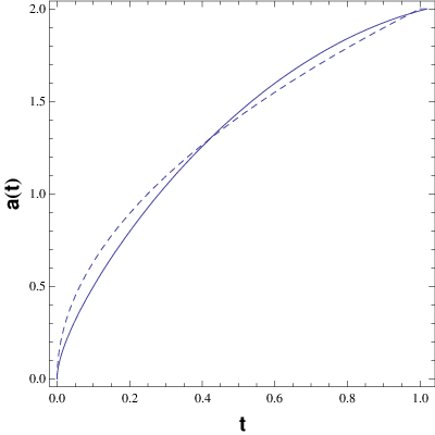
Imposing $0<q\leq 1$ and $1<n<2$, we see that $a\rightarrow a_{s0}$, $\dot{a}\rightarrow\frac{q(a_{s0}-1)}{t_{s0}}$ and $\ddot{a}\rightarrow\infty$, as $t\rightarrow t_{s0}$. Hence, the scale factor and its first derivative remain finite, implying that the density remains also finite, while the second derivative of the scale factor, and consequently the pressure, diverges. We assume the condition $0<q<1$ in order to have a decelerating universe as $t\rightarrow 0$, but this condition could be relaxed without affecting our results.

There is no exact solution for the Klein-Gordon equation for the form (4) for the scale factor. Therefore, we consider some simplifications. We divide the entire evolution of the universe into two phases: one which characterizes the primordial phase, $t\rightarrow 0,$ and other which characterizes the ”singular” phase, $t\rightarrow t_{s0}$. For the primordial phase, we will use the radiation-dominated phase of the standard model (i.e. $q=1/2$), for which it is possible to solve the Klein-Gordon equation so that the solution naturally contains the structure of the vacuum state of quantum fields.

Let us consider the asymptotic behaviours of the solution (4):

• •

  Primordial radiation phase ($t\rightarrow 0$):

  	$\displaystyle a$	$\displaystyle=$	$\displaystyle\frac{a_{s0}-1}{t_{s0}^{1/2}}t^{1/2},$		(7)
  	$\displaystyle\dot{a}$	$\displaystyle=$	$\displaystyle\frac{(a_{s0}-1)}{2\,t_{s0}^{1/2}}t^{-1/2}.$		(8)

• •

  Singular phase ($t\rightarrow t_{s0}$):

  	$\displaystyle a$	$\displaystyle=$	$\displaystyle a_{s0},$		(9)
  	$\displaystyle\dot{a}$	$\displaystyle=$	$\displaystyle\frac{(a_{s0}-1)}{2t_{s0}}.$		(10)

We introduce the conformal time, $\eta$, defined by $ad\eta=dt$ and re-express the scale factor during the radiative phase as $a=r\,t^{\frac{1}{2}}$, where the constant $r=\frac{a_{s0}-1}{\sqrt{t_{s0}}}$, so $\eta=\frac{2}{r}t^{\frac{1}{2}}.$This leads finally to the following expressions:

• •

  Primordial radiation phase ($\eta\rightarrow 0$):

  	$\displaystyle a$	$\displaystyle=$	$\displaystyle a_{0}\eta,$		(11)
  	$\displaystyle a^{\prime}$	$\displaystyle=$	$\displaystyle a_{0}.$		(12)

• •

  Singular phase ($\eta\rightarrow\eta_{s0}$):

  	$\displaystyle a$	$\displaystyle=$	$\displaystyle a_{s0},$		(13)
  	$\displaystyle a^{\prime}$	$\displaystyle=$	$\displaystyle\frac{a_{0}a_{s0}}{2\sqrt{t_{s0}}}.$		(14)

In the above expressions, $a_{0}=\frac{r^{2}}{2}$ and ${}^{\prime}=d/d\eta$. The transition to the singular phase now occurs at the conformal time $\eta=\eta_{0}$ and we have

$$a_{p}(\eta_{0})=a_{s}(\eta_{0}),\quad a_{p}^{\prime}(\eta_{0})=a_{s}^{\prime}(\eta_{0}),$$

(15)

where the subscripts $p$ and $s$ denote primordial and singular phases, respectively. This implies that

$$\eta_{0}=\frac{a_{s0}}{a_{0}}=\frac{2a_{s0}t_{s0}}{(a_{s0}-1)^{2}}\quad.$$

(16)

The matching conditions imply

$$a_{0}=\frac{a_{s0}}{\eta_{0}},\quad a_{s0}=2\sqrt{t_{s0}},$$

(17)

and the solutions for the two phases are:

1. 1.

   Primordial radiation phase:

   $$a=a_{s0}\frac{\eta}{\eta_{0}},\quad a^{\prime}=a_{0}=\frac{a_{s0}}{\eta_{0}};$$

   (18)

2. 2.

   Singular phase:

   $$a=a_{s0},\quad a^{\prime}=a_{0}=\frac{a_{s0}}{\eta_{0}}.$$

   (19)

In order to construct the simplified model of approach to a sudden singularity, we will consider $\eta_{0}$, $\eta_{s}$ and $a_{s0}$ to be independent free parameters.

In a spatially-flat Friedmann universe, the Klein-Gordon equation for a massless field, $\phi$, is

$$\Box\phi\equiv\phi^{\prime\prime}+2\frac{a^{\prime}}{a}\phi^{\prime}+k^{2}c^{2}\phi=0,$$

(20)

where we have re-inserted the light velocity, $c,$ and if $k$ is the wave number of the Fourier decomposition:

$$\phi(\eta,\vec{x})=\frac{1}{(2\pi)^{3/2}}\int\phi_{k}(\eta)e^{-i\vec{k}\cdot\vec{x}}d^{3}k.$$

(21)

For simplicity, we have omitted the Fourier index in the function $\phi$. Now, we scale by $H_{0}^{2}$, where $H_{0}$ is the Hubble parameter at the moment of the transition, $\eta_{0}$. Moreover, we define $\bar{k}=k\,l_{H}$, where $l_{H}$ is the Hubble radius at $\eta_{0}$. Note also that the scalar field has dimensions of (length)^1/2.

Now we consider the Klein-Gordon equation for the two phases defined above. For simplicity, we will omit the bars, setting $\bar{k}\rightarrow k$, and $H_{0}\eta\rightarrow\eta$ (a dimensionless time parameter). Note that with this parametrization, $\eta_{0}=1$ (since $H_{0}\eta_{0}=1$ in the old variables).

Using the solutions of the Klein-Gordon equation in the two phases, we match the fields and their first derivative at $\eta=\eta_{0}$. This gives the following expressions:

	$\displaystyle\sqrt{\frac{1}{2k}}e^{ik}$	$\displaystyle=$	$\displaystyle e^{-1}\biggr\{A_{+}e^{i\omega}+A_{-}e^{-i\omega}\biggl\},$		(38)
	$\displaystyle(-1+ik)\sqrt{\frac{1}{2k}}e^{ik}$	$\displaystyle=$	$\displaystyle A_{+}(-1+i\omega)e^{(i\omega-1)}-A_{-}(1+i\omega)e^{-(i\omega+1)}.$		(39)

Taking the combination $((1+i\omega)\times$(38) + (39), and later $((1-i\omega)\times$(38) + (39), we find:

	$\displaystyle A_{+}$	$\displaystyle=$	$\displaystyle\frac{1}{2\omega}\sqrt{\frac{1}{2k}}e^{[i(k-\omega)+1]}(\omega+k),$		(40)
	$\displaystyle A_{-}$	$\displaystyle=$	$\displaystyle\frac{1}{2\omega}\sqrt{\frac{1}{2k}}e^{[i(k+\omega)+1]}(\omega-k)].$		(41)

The energy density of the created particles is given by (see [14]),

$$\rho_{s}=\frac{\hbar H_{0}^{5}}{4\pi^{2}c^{6}a^{2}}\int_{0}^{\infty}dk\,k^{2}\biggr\{{\phi^{\prime}}_{k}{\phi^{\prime}}_{k}^{\ast}+k^{2}\phi_{k}\phi_{k}^{\ast}\biggl\}.$$

(42)

This expression is obtained by computing the vacuum expectation value of the Hamiltonian for a quantized massless scalar field. It is completely equivalent to the alternative derivation of the energy density using the Bogoliobov coefficients [7, 15]. The pressure associated to the created particles is given by [14]:

$$p_{s}=\frac{\hbar H_{0}^{5}}{4\pi^{2}c^{8}a^{2}}\int_{0}^{\infty}dk\,k^{2}\biggr\{{\phi^{\prime}}_{k}{\phi^{\prime}}_{k}^{\ast}-\frac{k^{2}}{3}\phi_{k}\phi_{k}^{\ast}\biggl\}.$$

(43)

Now, using (32) and (40,41), we find the following expression for the energy:

	$\displaystyle\rho_{s}$	$\displaystyle=$	$\displaystyle\frac{3}{2}\frac{\hbar\,H_{0}^{5}}{c^{6}}\frac{l_{pl}\,e^{y}}{4\pi^{2}a_{s}^{2}}\int_{0}^{k_{m}}dk\,\frac{4k}{k^{2}-1}\biggr\{(2k^{2}-1)k^{2}$		(44)
		$\displaystyle-$	$\displaystyle\cos[\sqrt{k^{2}-1}y]+\sqrt{k^{2}-1}\sin[\sqrt{k^{2}-1}y]\biggl\},$

where $y=2(1-\eta)$. The transition occurs at $\eta=\eta_{0}=1$ ($y=0$), noting the re-scaling. The upper limit of integration was set by $k_{m}$, an ultraviolet cut-off that must be identified with the Planck wavenumber. The reason for this is that we expect the Klein-Gordon equation may not retain its simple form (20) at energies higher than the Planck scale, where quantum gravity enters. There are many studies of the modification of the usual dispersion relation for a scalar field in the context of black hole thermodynamics and cosmological perturbations of quantum origin, two situations plagued by transplanckian frequencies - see [16] and references therein. The modification of the dispersion relation is usually treated by introducing a decreasing exponential term, which leads to a very important suppression in the integration in the transplanckian region. The adoption of this procedure is equivalent to stopping the integration near the Planck frequency. Since the extrapolation to the transplanckian regime is very speculative, we will ignore this transplanckian problem and adopt a more conservative regularisation procedure [15]. We will return to this problem later.

Let us choose the scaling so that $a_{s0}=1$. The above expressions can be then be rewritten as

	$\displaystyle\rho_{s}$	$\displaystyle=$	$\displaystyle\frac{l_{pl}^{3}}{l_{H}^{3}}\frac{\rho_{0}}{\pi}\,e^{y}\int_{0}^{k_{m}}dk\,\frac{4k}{k^{2}-1}\biggr\{(2k^{2}-1)k^{2}$		(45)
		$\displaystyle-$	$\displaystyle\cos[\sqrt{k^{2}-1}y]+\sqrt{k^{2}-1}\sin[\sqrt{k^{2}-1}y]\biggl\}\quad,$

where $\rho_{0}$ is the background cosmological density at the time of the transition.

This integral can be solved exactly and we have

	$\displaystyle\rho_{s}$	$\displaystyle=$	$\displaystyle 2\frac{l_{pl}^{3}}{l_{H}^{3}}\frac{\rho_{0}}{\pi}\,e^{y}\biggr\{k_{m}^{4}+k_{m}^{2}+\ln[k_{m}^{2}-1]-2Ci[-\sqrt{k_{m}^{2}-1}y]$		(46)
		$\displaystyle+$	$\displaystyle 2Chi[-y]-2\frac{\cos[\sqrt{k_{m}^{2}-1}y]}{y}+2\frac{\cosh y}{y}\biggl\}.$

In this expression, $Ci[x]$ is the cosine integral function and $Chi[x]$ is the hyperbolic cosine integral function.

The general behaviour indicates that the energy density of created particles decreases, see the bottom left graphic in figure 1. This expression is rigorously valid only after the transition. The initial condition is the number of particles created during the first (radiative) phase. The plot is made in units of this initial number, which is, at best, small. From this we can conclude that the sudden singularity is robust against particle production due to quantum effects, since the energy density of created particles is generally much smaller than the energy density of the background, and goes quickly to zero as the future singularity is approached. This result also confirms the self-consistency of our calculation using the Klein-Gordon equation to describe the evolution of a quantum field in the metric of a classical background cosmology [15].

If we now take the limit $k_{m}\rightarrow\infty$, keeping the Klein-Gordon equation in its traditional form (ignoring the transplanckian problems), we find that there is a quartic, a quadratic and a logarithmically divergent term. Moreover, the last term in the integral (44) may only ultimately have a meaning if it is treated as a distribution. Such divergencies may be removed using regularization of the energy-momentum tensor. The general result depends strongly on the background, which in our case is quite non-trivial. Even if we consider the simplified scenario with a radiative phase preceding a singular phase, the regularization could be implemented in the radiation-dominated phase (which is a known result [15]), but the existence of a discontinuity in the second derivative, due to the matching conditions we employ, makes the application of the usual expression neither direct nor simple. But, we can proceed in a more straightforward way. In the singular phase, we we are evaluating the creation of particles and the scale factor becomes constant. This makes it secure to use a covariant subtraction of the infinities [17], for the density and for the pressure,

$$<T_{\mu\nu}>_{reg}=<T_{\mu\nu}>_{0}-<T_{\mu\nu}>_{div}\quad,$$

(47)

where $<T_{\mu\nu}>_{reg}$ stands for the regularized energy-momentum tensor, $<T_{\mu\nu}>_{0},$ for the energy-momentum tensor evaluated using the expressions above, and $<T_{\mu\nu}>_{div}$ is its corresponding divergent part. The divergent parts are represented by the first term in (44). The final expression is given by (see the Appendix)

$$\rho_{s}=\frac{p_{s}}{3}=4\frac{l_{pl}^{3}}{l_{H}^{3}}\frac{\rho_{0}}{\pi}\,\biggr\{e^{y}\,\biggr[Chi[-y]+\frac{\cosh y}{y}\biggl]\biggl\}.$$

(48)

It is very important to stress that the Minkowski limit, obtained by imposing $\mathbf{\rho}_{0}\rightarrow 0$, leads to a null result, the same as we would obtain if we had computed the vacuum expectation value in Minkowski space-time and subtracted the divergencies. At same time, the resulting energy-momentum is conserved. This confirms the consistency of the procedure employed above. Note that, in the present case, the equation of state does not coincide with the classical equation of state of a massless scalar field in a FRW background, which is that of a stiff matter fluid ($p=\rho$). In general, the quantization of a classical system may change the classical equation of state. The general form of the regularized energy density of created particles is exhibited in figure $1$, showing a decreasing behavior as before.

It is possible to obtain at least some information about the effects of using a simplified model, where the evolution of the universe is described by two phases, by integrating numerically the exact Klein-Gordon equation using (4,5). The results are of course plagued by the problem of the ultraviolet divergence. But, we can stop the integration at a high frequency and compare the result with the expression (46), or even with (48). The initial condition is given by the same vacuum state that we used above. The results for the background and for the energy density of particles created are compared in figure $1$, where we have also inserted the expressions for the energy of the produced particles using the Planck frequency cut-off (46) and the regularized energy-momentum tensor (48) as well as the numerical computation. Of course, the regularized expression (48) fits the numerical integration only in a general form; this is natural since a divergent contribution has been extracted to obtain (48). Yet they agree in the sense that both predict a decreasing energy of produced particles as the singularity is approached. This is a quite general behavior that remains even if the free parameters, like $a_{s0}$ and $H_{0}$, are varied. As is also expected, the numerical fitting to the simplified analytical expression is better when the duration of the singular phase is small compared to that of the preceding radiative phase. Moreover, the numerical integration reveals the effect of the sharp transition (which is not displayed in the figures): in (46,48) there is a divergence in the energy at $y=0$, which does not appear in the numerical computation. This is an effect of the discontinuity in the second derivative, which is clearer when the Klein-Gordon equation is written as in (34).

To obtain more details of the result described above, we can use the expression for the particle production exhibited in reference [15]. The energy density can be written as

$$\rho_{s}=\frac{\hbar c}{a}\int_{0}^{\infty}N_{k}k\,d^{3}k,$$

(49)

where $N_{k}$ is the particle occupation number. Comparing with (45), and retaining only the relevant terms after regularization, the particle occupation is then given by

$$N_{k}\propto\frac{e^{y}}{k^{2}(k^{2}-1)}\biggr\{(-\cos[\sqrt{k^{2}-1}y]+\sqrt{k^{2}-1}\sin[\sqrt{k^{2}-1}y]\biggl\}.$$

(50)

From this expression we can verify that the particle production decreases as the sudden singularity is approached, in contrast to what happens in the case of approach to a ’big rip’ future singularity [18] (where $a\rightarrow\infty,\rho\rightarrow\infty$ and $\left|p\right|\rightarrow\infty$ as $t\rightarrow t_{s}$). Moreover, light particles are produced more copiously than heavy particles, as would be expected. These behaviors are shown in Figure 2.

We can try to compare our results with those obtained in reference [8]. However, the context is quite different to that of this paper since the authors of [8] have considered an ensemble of conformal quantum fields, (whereas we consider only a non-conformal, massless scalar field), generating a trace anomaly by using the effective-action approach where gravity is modified by requiring that the quantum fields must be renormalisable on a given metric background. They find that the sudden singularity can be modified by quantum effects. The energy conditions could be violated and a big-rip singularity ensue. In our calculation, these quantum effects are inoperative. A possible reason for these differences is the expression used in ref. [8] for the conformal anomaly: it was derived near an initial strong curvature singularity ($a\rightarrow 0,\dot{a}/a\rightarrow\infty,\rho\rightarrow\infty$ as $t\rightarrow 0$). Since the scale factor becomes constant near the sudden singularity ($a,\dot{a},\rho$ all finite but $\ddot{a}\rightarrow\infty$ as $t\rightarrow t_{s}$), it is possible that the expression used for the conformal anomaly does not apply unchanged from its form in a scenario with a dynamic scale factor near an initial singularity where the density diverges. The quantum effects considered in reference [8] have their natural domain of applicability in the early universe, near the big bang rather than at a late-time sudden singularity where geodesics are undisturbed. At a future sudden singularity there is a curvature singularity which can in principle justify the employment of a conformal anomaly for the sudden singularity. However, the sudden singularity has many features which distinguish it from the initial big bang singularity: the divergence appears only in the second derivative of the scale factor (or, equivalently, in the pressure) and the expansion rate and the density remain finite. Hence, the validity of such an extrapolation to the sudden singularity remains to be proven. In particular, if particle production effects from other type of fields, like massive or conformal scalar fields, or even vectorial and spinorial quantum fields, produce such a large back-reaction that a sudden singularity is changed into a big rip singularity then it is difficult to describe that self-consistently in terms of effective quantum stresses on a fixed background because the background expansion is strongly perturbed.

We have considered the quantum particle production that would occur in an isotropic and homogeneous universe on approach to sudden singularity, where $a,\dot{a}$ and $\rho$ remain finite while $\ddot{a}$ and $p$ diverge. If significant, such quantum effects could modify or remove a sudden singularity at finite time. We have set up a simple exactly soluble model in which an early radiation-dominated universe evolves towards a sudden singularity at finite time. We compute the quantum particle production as the singularity is approached and show that its effects remain negligible with respect to the classical background pressure and density all the way into the singularity. We compare our results to other discussions of quantum effects in the literature; we argue that any effects created by the presence of small anisotropies will be negligible and show how a simple classical description of the quantum particle production as an effective bulk viscosity in a Friedmann universe gives a similar outcome.

The energy density and the pressure are given by (neglecting multiplicatively unimportant terms),

	$\displaystyle\rho_{s}$	$\displaystyle=$	$\displaystyle\frac{1}{a^{2}}e^{y}\int_{0}^{\infty}\frac{k}{\omega^{2}}\biggr\{(2k-1)k^{2}-\cos(\omega y)+\omega\sin(\omega y)\biggl\}dk\quad,$		(52)
	$\displaystyle p_{s}$	$\displaystyle=$	$\displaystyle\frac{1}{a^{2}}e^{y}\int_{0}^{\infty}\frac{k}{\omega^{2}}\biggr\{(2k-1)\frac{k^{2}}{3}-\biggr(1-\frac{2}{3}k^{2}\biggl)\cos(\omega y)+\omega\sin(\omega y)\biggl\}dk\quad.$		(53)

In these expressions, $\omega=\sqrt{k^{2}-1}$ and $y=2(1-\eta)$ where $\eta$ is the conformal time (which is proportional to the cosmic time $t$ when $a=$ constant). Now, let us consider the conservation law,

$$\rho^{\prime}+3\frac{a^{\prime}}{a}(\rho+p)=0\quad.$$

(54)

The primes mean derivative with respect to $\eta$. This may be rewritten, after redefining the time variable using the (constant) Hubble parameter, in terms of the derivative with respect to $y$:

$$-2\dot{\rho}+3(\rho+p)=0\quad.$$

(55)

It is easy to see that the expressions (46,52) satisfy (55). It is important to note that, even if $a$ is constant, we must derive it since $\dot{a}$ (equivalently, $a^{\prime}$) is not zero, being also equal to a constant. More importantly, if we rewrite (46,52) as

	$\displaystyle\rho_{s}$	$\displaystyle=$	$\displaystyle\rho_{s1}+\rho_{s2}\quad,$		(56)
	$\displaystyle p_{s}$	$\displaystyle=$	$\displaystyle p_{s1}+p_{s2}\quad,$		(57)

where

	$\displaystyle\rho_{s1}$	$\displaystyle=$	$\displaystyle\frac{1}{a^{2}}e^{y}\int_{0}^{\infty}\frac{k}{\omega^{2}}(2k-1)k^{2}\,dk\quad,$		(58)
	$\displaystyle\rho_{s2}$	$\displaystyle=$	$\displaystyle\frac{1}{a^{2}}e^{y}\int_{0}^{\infty}\frac{k}{\omega^{2}}\biggr\{-\cos(\omega y)+\omega\sin(\omega y)\biggl\}dk\quad,$		(59)
	$\displaystyle p_{s1}$	$\displaystyle=$	$\displaystyle\frac{1}{a^{2}}e^{y}\int_{0}^{\infty}\frac{k}{3\omega^{2}}(2k-1)k^{2}\,dk\quad,$		(60)
	$\displaystyle p_{s2}$	$\displaystyle=$	$\displaystyle\frac{1}{a^{2}}e^{y}\int_{0}^{\infty}\frac{k}{\omega^{2}}\biggr\{-\biggr(1-\frac{2}{3}k^{2}\biggl)\cos(\omega y)+\omega\sin(\omega y)\biggl\}dk\quad,$		(61)

then the pairs ($\rho_{s1},p_{s2}$) and ($\rho_{s1},p_{s2}$) satisfy (55) separately.

Now we can easily show that $\rho_{s2}$ is finite. In fact,it can be written as

$$\rho_{s2}=-\frac{1}{a^{2}}\frac{d}{dy}\int_{0}^{\infty}\frac{k\,dk}{\omega^{2}}\biggr[e^{y}\cos(\omega y)\biggl]\quad.$$

(62)

The integral can now be performed, leading to

$$\rho_{s2}=\frac{1}{a^{2}}\frac{d}{dy}\biggr(e^{y}Chi(-y)\biggl)\quad,$$

(63)

where we have exploited the fact that the cosine function is even in its argument. This function is finite, except at $y=1$, an effect of the sharp transition of the second derivative in the simplified model which does not appear in the numerical integration, where the background is smooth.

Now we can obtain the pressure $p_{s2}$. The result is

$$p_{s2}=\frac{1}{3}\frac{e^{y}}{a^{2}}\biggr\{Chi(-y)+3\frac{\cosh y}{y}-2\frac{\cosh y}{y^{2}}+2\frac{\sinh y}{y}\biggl\}\quad,$$

(64)

which goes to zero asymptotically.

Hence, after subtracting the divergent parts $\rho_{s1}$ and $p_{s1}$, we obtain finite expressions for the energy and for the pressure, which have the ordinary Minkowski space-time limit satisfying the covariant energy-momentum conservation law.

The regularization procedure is employed here is inspired in the $n$-wave technique [19] (see also [23]). Here, its application is very simple due to the natural splitting of the energy density and pressure into a divergent and a finite parts, which separately satisfy the conservation law.

References

- [1] J.D. Barrow, Class. Quantum Gravity 21, L79 (2004).
- [2] J.D. Barrow, Class. Quantum Grav. 21, 5619 (2004).
- [3] J.D. Barrow, G.J. Galloway and F.J. Tipler, Mon. Not. Roy. astr. Soc., 223, 835 (1986); J.D. Barrow, Phys. Lett. B 235, 40 (1990).
- [4] Y. Shtanov and V. Sahni, Class, Quantum Grav. 19, L101, (2002); J.D. Barrow and C.G. Tsagas, Class. Quantum Grav. 22, 1563 (2005); M.P. Dabrowski, Phys. Rev. D 71, 103505 (2005); S. Nojiri, and S.D. Odintsov, arXiv:hep-th/0412030v1.
- [5] S. Nojiri, S.D. Odintsov and S. Tsujikawa, Phys. Rev. D 71, 063004 (2005); C. Cattoen and M. Visser, Class. Quantum Grav. 22, 4913 (2005), M. Dabrowski, Phys. Lett. B 625, 184 (2005); H. Stefancic, Phys. Rev. D 71, 084024 (2005).
- [6] M.P. Dabrowski, T. Denkiewicz and M.A. Hendry, arXiv:gr-qc/0704.1383.
- [7] A.B. Batista, J.C. Fabris and S. Houndjo, Gravitation & Cosmology 14, 140 (2008).
- [8] S. Nojiri, S.D. Odintsov, Phys. Lett. B 595, 1 (2004)
- [9] R. Penrose, The Road to Reality, Jonathan Cape, London (2004).
- [10] L. Fernandez-Jambrina and R. Lazkoz, Phys. Rev. D 70, 121503(R) (2004) and L. Fernandez-Jambrina and R. Lazkoz, Phys. Rev. D 74, 064030 (2006); K. Lake, Class. Quantum Grav. 21, L129 (2004); A. Balcerzak and M.P. Dabrowski, Phys. Rev. D 73, 101301 (2006).
- [11] M. Sami, P. Singh and S. Tsujikawa, Phys. Rev. D 74, 043514 (2006); S. Cotsakis and I. Klaoudatou, J. Geom. Phys. 57, 1303 (2007).
- [12] J.D. Barrow, Phys. Lett. B 180, 335 (1987); J.D. Barrow, Nucl. Phys. B 310, 743 (1988); J.D. Barrow, in The Formation and Evolution of Cosmic Strings, eds. G. Gibbons, S.W. Hawking & T. Vaschaspati, , CUP, Cambridge (1990), pp. 449-464.
- [13] L. Grishchuk, Sov. Phys. JETP 40, 409 (1975).
- [14] A. Guangui, J. Martin and M. Sakellariadou, Phys. Rev. D66, 083502 (2002).
- [15] N.D. Birrell and P.C.W. Davies, Quantum Fields in Curved Space, CUP, Cambridge (1982).
- [16] M. Lemoine, M. Lubo, J. Martin and J-Ph. Uzan, Phys. Rev. D65, 023510 (2002) .
- [17] L.H. Ford, Phys. Rev. D14, 3304 (1976).
- [18] R.R. Caldwell, Phys. Lett. B 545, 23 (2002).
- [19] Y.B. Zeldovich and A.A. Starobinskii, Sov. Phys. JETP 34, 1159 (1972), Y.B. Zeldovich, in Confrontation of Cosmological Theories with Observation, ed. M.S. Longair Reidel, Dordrecht (1974), pp.329-333; B.L. Hu, Phys. Lett. B 108, 19 (1982).
- [20] V.N. Lukash and A.A. Starobinskii, Sov. Phys. JETP 39, 742 (1974).
- [21] J.C. Fabris, A.M. Pelinson, Nucl. Phys. B597, 539 (2001).
- [22] A.A. Starobinskii, Phys. Lett. B 91, 99 (1980).
- [23] Yu. V. Pavlov, Theor. Math. Phys. 138, 383 (2004).