Dissipation and nonlocality in a general expanding braneworld universe
Abstract
We study the evolution of both scalar and tensor cosmological perturbations in a Randall-Sundrum braneworld having an arbitrary expansion history. We adopt a four dimensional point of view where the degrees of freedom on the brane constitute an open quantum system coupled to an environment composed of the bulk gravitons. Due to the expansion of the universe, the brane degrees of freedom and the bulk degrees of freedom interact as they propagate forward in time. Brane excitations may decay through the emission of bulk gravitons which may escape to future infinity, leading to a sort of dissipation from the four dimensional point of view of an observer on the brane. Bulk gravitons may also be reflected off of the curved bulk and reabsorbed by the brane, thereby transformed into quanta on the brane, leading to a sort of nonlocality from the four dimensional point of view. The dissipation and the nonlocality are encoded into the retarded bulk propagator. We estimate the dissipation rates of the bound state as well as of the matter degrees of freedom at different cosmological epochs and for different sources of matter on the brane. We use a near-brane limit of the bulk geometry for the study when purely nonlocal bulk effects are encountered.
1 Introduction
Randall and Sundrum introduced a braneworld model with an infinite extra dimension [1] where our observable universe is a four dimensional hypersurface, the brane, embedded into a five dimensional Anti-de Sitter () bulk spacetime. The curved geometry of space induces an effective compactification in the extra dimension through its curvature radius and thus prevents four dimensional (4d) gravity from leaking into the extra dimension. Consequently, standard 4d Einstein gravity is recovered at large distances on the brane. Corrections to the Newton square inverse force law arise at scales smaller than [2] (in current experimental tests of Newton’s law, [3]). Spatially homogeneous and isotropic cosmological background solutions in the Randall-Sundrum (RS) model have been found [4]. These solutions include an additional term quadratic in the energy-momentum tensor in the Friedmann equation, causing significant modifications of the standard cosmology at high density. In the language of string theory, all the Standard Model fields are confined to the brane. Only the gravitons propagate in the entire bulk spacetime. It is hoped that the presence of an infinite extra dimension may be tested by cosmological observations, such as the measurements of temperature and polarization anisotropies of the Cosmic Microwave Background (CMB).
Cosmological perturbation theory about the cosmological background is an essential tool to probe the presence of extra dimensions. In braneworlds, cosmological perturbation theory is more complicated than in standard 4d cosmology because the brane breaks the 5d spatial homogeneity and isotropy of the bulk. Consequently, the linearized equations are no longer ordinary differential equations (ODE) in time but become partial differential equations (PDE) in time and the extra dimension. Analytic solutions to cosmological perturbations have however been found for the maximally symmetric cases of a Minkowski brane or a pure de Sitter brane [1], [5]. In these special cases of higher symmetry the spectrum of 5d gravitons includes one discrete mode bound to the brane (if the bulk is -symmetric) and a continuum of free modes. From the point of view of an observer on the brane, the bound state is interpreted as the 4d massless graviton and reproduces standard 4d Einstein gravity on the brane. The continuum is interpreted as 4d massive Kaluza-Klein (KK) gravitons whose interaction with the brane degrees of freedom is suppressed at low energy. In order to explore observational signatures for the presence of extra-dimensions, it is necessary to compute the evolution of cosmological perturbations in the more realistic case of a brane having a time-dependent stress-energy, i.e. a Friedmann-Robertson-Walker (FRW) brane, for instance with an inflation era followed by a radiation/matter dominated era. Several formalisms exist for evolving linearized perturbations in a braneworld scenario [7]. Here we use the formalism of Mukohyama [8]. The main difficulty is that, except for the case of an uniformly accelerated brane (flat brane or de Sitter brane) where analytical solutions have been obtained, the equations are generally not separable because of the complicated motion of the expanding brane in the bulk (a review on cosmological perturbations in expanding braneworlds is given in reference [12]). This problem has been investigated numerically and a number of interesting results have been obtained [14, 15, 16, 17, 18, 19, 20, 21, 22]. The braneworld perturbations problem is in principle entirely solvable numerically once the initial vacuum in is known. However the specification of initial conditions in the bulk poses a problem of more fundamental nature. There is no unique physically motivated choice of initial conditions for an bulk background [24, 25] (quite unlike the situation for space). Consequently the results of these numerical studies are subject to certain assumptions concerning the initial conditions.
Five dimensional transverse and traceless metric fluctuations describe the true bulk gravitational waves (5d gravitons) and contain five degrees of freedom (d.o.f). By "projecting" the five d.o.f onto a flat static brane, they split into tensor perturbations (the two d.o.f of the 4d graviton), vector perturbations (the two d.o.f called "graviphotons") and scalar perturbations (one d.o.f called "graviscalar"), in a representation. This "projection" is somewhat ambiguous in the case of an arbitrary motion of the cosmological brane. In this case it is more convenient to use directly the symmetry of the unperturbed spacetime to decompose the linear perturbations into tensor, vector and scalar perturbations. The advantage of this decomposition is that scalar, vector and tensor perturbations evolve independently at linear order. Tensor perturbations are transverse and traceless and are the easiest to deal with. They correspond to 4d gravitational waves and propagate freely into the bulk, independently of the presence of matter on the brane. By definition tensor perturbations are automatically gauge-invariant at linear order. Their wave function obeys an equation similar to a Klein-Gordon equation for a massless scalar field minimally coupled to gravity. The Israel junction conditions reduce merely to Neumann boundary conditions on the brane. Vector and scalar metric perturbations are more complicated to deal with because of their coupling to matter on the brane. Mukohyama has shown that, in the absence of matter in the bulk, scalar (as well as vector) perturbations in the "5d longitudinal" gauge can be derived from a single scalar master field, which obeys a five dimensional wave equation [8] (see also [9]). For vector perturbations, the boundary conditions for the master field are Dirichlet boundary conditions. In the more interesting case of scalar perturbations, the master field satisfies more complicated "nonlocal" boundary conditions on the brane11 1 The term “nonlocal” for the boundary conditions has nothing to do with the nonlocality studied in this paper which is due to the information coming from the bulk. As it was stressed in [6], the terminology “nonlocal” for the boundary conditions is not appropriate, although it is frequently used in the literature, because they contain only a finite number of derivatives.. Some authors have shown the connection between the master field formalism and the formalisms in different gauges [10]. Although there has been progress in braneworld cosmological perturbation theory, there are a few quantitative predictions for the evolution of cosmological perturbations in expanding braneworlds.
In this paper we study the evolution of cosmological perturbations of a FRW brane having an arbitrary motion in the bulk. The goal of this work is to estimate the order of magnitude of the extra dimensional effects. Instead of looking for exact solutions to the perturbation equations, we are primarily interested in the role of the bulk gravitons in the brane-bulk interaction, following the ideas developed in the article of Binetruy, Bucher and Carvalho [26]. When the Hubble parameter on the brane changes with time, the acceleration of the brane in the bulk also changes and gravitons are emitted into the bulk. These may escape to future infinity or they may be reabsorbed by the brane because of reflections of the emitted gravitons off of the curved bulk. From the point of view of an observer on the brane, these processes appear to generate dissipation and nonlocality [26]. Here these bulk induced effects are encoded into the retarded bulk propagator, which is systematically inserted into the effective brane propagator by doing a resummation of the bulk backreaction effects at all order in the brane-bulk coupling. The approach used in this work is a four dimensional perspective that regards the degrees of freedom localized on the brane universe as an open quantum system coupled to a large environment composed of the bulk gravitons. In the language of non-equilibrium quantum field theory, the bulk propagator plays the same role as a self-energy, dressing the bare fields composed of the discrete degrees of freedom localized on the brane. In this work we estimate the magnitude of the decay rate of the graviton bound state by studying the evolution of tensor perturbations in the frame of a cosmological brane with an arbitrary expansion history embedded in a -symmetric space. Some authors obtained analytical results for the order of magnitude of the modified power spectrum for tensor perturbations, in the simplified braneworld model where the Hubble factor on the brane changes instantaneously [11]. Here we consider a more realistic model where the Hubble factor changes continuously and adiabatically in the sense that . We also work out the dissipation of purely localized brane degrees of freedom, such as an adiabatic perfect fluid or a slowly rolling scalar field on the brane, by studying the evolution of scalar cosmological perturbations and the coupling between metric and matter perturbations. We use Gaussian normal (GN) coordinates, where the extra dimensional coordinate measures the proper distance from the brane and the position of the brane in the bulk is fixed. GN coordinates have also the advantage of simplifying the form of the perturbed boundary conditions on the brane. The main drawback of GN coordinates is the presence of coordinate singularities in the bulk at a finite distance from the brane, despite the bulk space being regular and extendable beyond the singularity by choosing another set of coordinates. Because of the arbitrary motion of a FRW brane in space, the metric components in GN coordinates have a complicated form which renders the equations of motion not separable. That is why we use a near-brane limit to perform the separation, actually only when purely nonlocal interactions arise between the bulk degrees of freedom and the brane degrees of freedom that are considered. This limit can be legitimized in the Randall-Sundrum model because the support of the wave function of the bound state is localized near the brane. We think that physics near the brane is suitable to describe dissipative effects in braneworlds. In order to focus our attention on the dissipative effects, we may approximate at high energy () the inhomogeneity of the bulk responsible for backscattering of gravitons in the bulk and subsequent nonlocal effects on the brane. This approximation is discussed in section 6.1.
The paper is organized as follows. In section 2 we introduce the dissipative and nonlocal effects which appear in braneworld cosmology and we present the self-energy approach used in the paper to study these effects. In section 3 we briefly recall the cosmological perturbation theory in braneworlds. In section 4 we explore the scalar perturbations and the brane-bulk interaction for a slowly rolling scalar field on the brane. We apply our method to compute the local dissipation rate of the inflaton perturbation due to the interaction with the bulk. In section 5 we compute the Gaussian normal metric of space with general Friedmann-Robertson-Walker (FRW) slices and present the near-brane limit of this geometry, which will be used as an approximation to evaluate the nonlocal corrections arising in the brane-bulk systems considered in the next sections. In section 6 we study the tensor perturbations and compute the dissipation rate of the graviton bound state. In section 7 we study the scalar perturbations for an adiabatic perfect fluid on the brane. We present our conclusions in section 8.
2 Dissipation and nonlocality in the expanding braneworld
Cosmological perturbations theory for the Randall-Sundrum model has been solved analytically for special brane universes where the Hubble factor on the brane is constant. In these cases the four dimensional universe is static () or follows a uniform expansion (). In the first case the Minkowski brane is at rest with respect to the five dimensional Anti-de Sitter () bulk, whereas in the second case the pure de Sitter () brane follows a uniformly accelerating trajectory in the bulk. The equations for the perturbations may be reduced to a Schrödinger-like equation. The presence of the brane within the bulk creates a -function potential well, while the curvature of the bulk creates a decreasing barrier potential (Fig. 1).

The resulting volcano-like potential gives rise to a single brane bound mode, the zero mass mode , in the spectrum of the linearized Einstein equations, surrounded by a continuum of massive Kaluza-Klein free modes, with for a brane [5]. The zero mode represents the standard massless graviton and reproduces the four dimensional gravity on the brane. The amplitude of the massive gravitons is suppressed near the brane at low energy due to the barrier potential.
Because of the presence of matter in the universe, the cosmological expansion history is no longer uniform. The Hubble parameter changes with time, inducing a change in the shape of the potential. Consequently, the brane degrees of freedom and the bulk degrees of freedom interact thus generating transitions between the modes.
The brane-bulk system is a Hamiltonian quantum system, which is necessarily conservative because the phase space density must be preserved under time evolution. In this sense, the brane-bulk system is intrinsically non-dissipative, and the appearance of dissipation can arise only as the result of “coarse graining”. The interaction between the quanta due to the expansion of the brane may be characterized by a Bogoliubov transformation ( matrix for a linear system) relating the modes of positive and negative frequency for the initial “in” vacuum and the resulting “out” vacuum. However, from the point of view of an observer confined to the brane, the four dimensional universe as a submanifold is an open quantum system. Consequently, the mixing between the modes localized on the brane and the delocalized modes in the bulk creates the appearance of dissipation to a four dimensional observer unable to access the bulk modes. The observer on the brane is sensitive only to a part of the complete vacuum, composed of only the discrete modes localized on the brane. We call this part “brane vacuum”. The Hilbert space is truncated because of dimensional reduction, and the “bulk vacuum”, composed of the continuous bulk modes, holds the missing information. When we observe the cosmological perturbations today, we measure expectation values of observables quadratic in the creation and annihilation operators for the modes localized on the brane today, namely and . The matrix expresses the “out” operators as linear combinations of and on one hand, and of and on the other. A useful parameterization of this transformation has been proposed in [26]. The authors require that and be entirely on the brane and in the bulk, respectively, and be normalized such that . Then may be expressed in terms of these according to one of the three following possibilities: either
| (1) |
where ; or
| (2) |
where ; or
| (3) |
where . may be constructed entirely as a linear combination of and , and likewise may be constructed entirely as a linear combination of the and the , being the index for the continuum modes. We observe in (3) that the bulk initial state may have a very important, or even dominant, role in determining what we see on the brane today.
However it has been numerically observed in [19] that the evolution of tensor perturbations on the brane today does not show any significant dependence on the bulk initial state when a -invariant initial vacuum is specified in the bulk, that is defined in a -slicing frame. However we might suspect that the initial amplitude of bulk modes that are initially located outside the bulk Cauchy horizon of the -slicing will not be suppressed when they causally affect the decelerating brane in the future. The relative contribution of the brane initial conditions and the bulk initial conditions in determinining what we see on the brane today should depend on the basis decomposition of the in-vacuum as described in (3). The main problem is that there are no natural initial conditions for [24, 25]: in standard inflation the backgound geometry is so the timelike geodesics diverge forward in time losing causallity such that initial irregularities become swept out, space thus exhibits natural initial conditions for generating homogeneity and isotropy. Whereas in Randall-Sundrum branewords the background geometry is so that the timelike geodesics first diverge and then refocus forward in time, thus conserving the initial amplitude of metric perturbations.
The brane-bulk interaction may be summarized by the following fundamental processes from the four dimensional point of view illustrated in Fig. 2. An initial vacuum state may be completely characterized by specifying the quantum state of the incoming gravitons on the past Cauchy horizon in the bulk and of the degrees of freedom on the brane at the intersection of the brane with . Subsequently, the bulk and the brane degrees of freedom interact as they propagate forward in time. Bulk gravitons may be absorbed and transformed into quanta on the brane. Similarly, brane excitations may decay through the emission of bulk gravitons. These may either escape to future infinity, leading to dissipation from the four dimensional point of view, or may be reabsorbed by the brane due to the bulk curvature, leading to nonlocality from the four dimensional point of view.
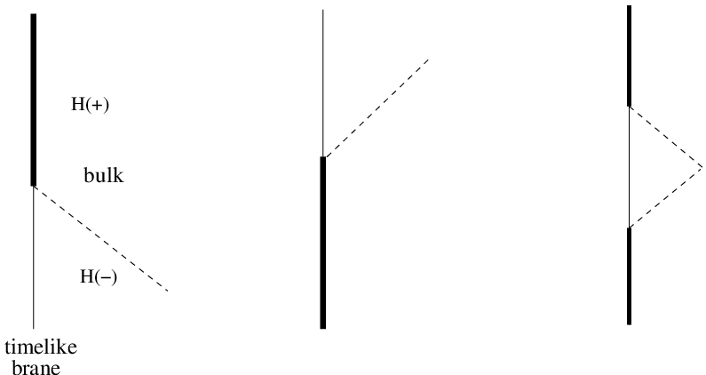
We may consider the brane-bulk interaction from the four dimensional perspective by regarding the brane degrees of freedom as an open quantum system coupled to an environment with a large number of degrees of freedom. Schematically, we may block diagonalize by Fourier transforming in the three transverse spatial dimensions. For an expanding braneworld with a perfect fluid or scalar field on the brane, the interaction between the scalar brane degree of freedom and a scalar bulk degree of freedom may be represented by a system of coupled equations. Under the approximations presented in detail later in the paper, this system of coupled equation may be written according to the general form
| (4) | |||||
| (5) | |||||
| (6) |
where and are polynomials in of degree one and degree two respectively, with time dependent coefficients. The first equation is the bulk equation of motion, the second the boundary condition on the brane, and the third the equation of motion for the brane degree of freedom. The brane and the bulk degrees of freedom are related according to
| (7) | |||||
| (8) |
where is the bare22 2 By “bare” we mean the propagator of the free brane fields excluding the interaction with the bulk. retarded brane propagator and is the Neumann form of the retarded bulk propagator. Due to the interaction, the effective retarded brane propagator may be obtained by resumming the infinite geometric series at all orders of the bulk backreaction
| (10) | |||||
| (11) |
where the bulk propagator links two points both lying on the brane. The brane degree of freedom is governed by the integro-differential equation
| (12) |
Here the bulk kernel is given by
| (13) |
and plays the role of a self-energy, dressing the bare field on the brane. Both the local dissipative effects and the nonlocal effects due to the interaction with the extra dimension are contained in this self-energy kernel. The bare retarded brane propagator is the propagator of an oscillator localized on the brane and accounts only for the transitions between the four dimensional modes due to the expansion of the universe.
We consider as an illustration the following couplings
| (14) |
Since the Neumann retarded bulk propagator on the brane can be written in the form
| (15) |
the bulk kernel may be decomposed into singular and regular parts
| (16) |
where
| (17) | |||||
| (18) |
The singular part is responsible for the local dissipative processes and the regular part describes subsequent nonlocal processes, such as reflections from the inhomogeneous curved bulk. The infinite summation
| (19) | |||||
| (20) |
is equivalent to adding a local dissipation term to the equation of motion for the brane degree of freedom. The infinite summation
| (22) | |||||
adds the nonlocality to the equation of motion such that the brane degree of freedom propagates as
| (23) |
Since a local singular part does not depend on the curvature of the background, the term which appears in the local dissipation rate may be replaced by the Neumann form of the Minkowski propagator. We recall that the Minkowski propagator is
| (24) |
where is the momentum in the three transverse spatial dimensions. Then and the local dissipation rate depends only on the couplings
| (25) |
For certain derivative couplings, additional local terms may appear leading for instance to a phase shift. There might also be a nonlocal dissipation term when there is no derivative in the couplings. This formalism with Green functions is useful to discriminate transitions among four dimensional brane modes due to the expansion of the universe from transitions between the brane and the bulk modes due to the presence of an extra dimension. Moreover this formalism allows us to distinguish the local dissipation processes from the nonlocal processes.
The purpose of this work is to estimate the dissipation rates of certain degrees of freedom confined to the brane or localized near the brane from an arbitrary expansion history of a brane having no special symmetries.
3 Braneworld cosmological perturbations
In this section we recall briefly the cosmological perturbations equations in braneworlds and the formalism of Mukohyama frequently used in the literature [6, 8, 9, 10, 13, 21, 16, 22]. The metric perturbations about the general bulk background metric , in Gaussian normal coordinates, given by
| (26) |
describe the five dimensional bulk gravitons. The evolution of these bulk perturbations (where we assume ) will depend on the coupling to the matter perturbations localized on the brane at through the linearized Einstein equations
| (27) |
from which linearized Israel junction conditions on the brane can be derived. The coupling is related to the five dimensional Planck mass , where is the four dimensional gravitational coupling constant and the curvature radius of the bulk space in the Randall-Sundrum model. The bulk metric perturbations can be decomposed into scalar, vector, and tensor perturbations.
3.1 Tensor perturbations
The gravitational waves away from the brane propagate freely in the bulk and independently of the presence of matter on the brane. They are described by transverse and traceless tensor perturbations of the metric
| (28) |
Tensor perturbations are gauge invariant at linear order and they do not couple to matter on the brane. The tensor perturbations are exactly described by a minimally coupled massless scalar field , Fourier transformed in the three transverse spatial dimensions, as
| (29) |
which propagates in the bulk background according to the Klein-Gordon equation
| (30) |
The Israel junction conditions reduce to a Neumann boundary condition on the brane
| (31) |
This boundary condition is homogeneous under the assumption that there are no anisotropic stresses on the brane.
3.2 Scalar perturbations
The scalar perturbations of the bulk background metric may be simplified by choosing a particular gauge knowned as “5d longitudinal gauge”. In this gauge there are four gauge-invariant variables and the line element is
| (33) | |||||
These five dimensional scalar metric perturbations couple to the four dimensional scalar matter perturbations on the brane, which are defined in the same gauge on the brane by33 3 We have neglected the scalar anisotropic stress which do not arise when considering the perturbations of a perfect fluid or a scalar field.
Here the greek indices label the four dimensions on the brane and the latin indices label the three transverse spatial dimensions on the brane. Throughout the paper, and denote respectively the energy density and the pressure of the effective matter on the brane as opposed to the real matter on the brane labeled by a subscript and related to the previous one by , , where is the brane tension, fine-tuned in the Randall-Sundrum model so that [1]. Mukohyama [8] (see also [9]) has shown that in the absence of bulk matter perturbations, the scalar metric perturbations in 5d longitudinal gauge can all be generated from a single scalar ‘‘master’’ field44 4 It should be noted that . according to
| (34) | |||||
| (35) | |||||
| (36) | |||||
| (37) |
The master variable satisfies the five dimensional wave equation
| (38) |
The Israel junction conditions reduce to the following "nonlocal" boundary conditions on the brane [13]
| (39) | |||||
| (40) | |||||
| (42) | |||||
4 Scalar perturbations: slow-roll inflaton on the brane
In this section we work out scalar metric and matter perturbations for a scalar field on the brane with a slow-roll potential, , such that the induced geometry on the brane is quasi-de Sitter. During slow-roll inflation the expansion of the universe is adiabatic in the sense that . The inflaton scalar field, , may be characterized by an energy density and a pressure
| (43) | |||||
| (44) |
We may combine the equations of Mukohyama presented in section 3.2 for scalar perturbations to obtain simple coupled equations of the brane-bulk system. Following the calculations done in [16, 22], we introduce the Mukhanov-Sasaki variable as the brane degree of freedom:
| (45) |
where is the perturbation of the inflaton and is one of the scalar metric perturbations, namely the curvature perturbation (37), projected on the brane. The equations of the brane-bulk system in the general Gaussian normal coordinate system (26) are then given by [16, 22]
| (46) | |||||
| (47) | |||||
| (48) |
where is the transverse momentum and the source is given by
The brane-bulk equations (46), (51) may be simplified for slow-roll inflation as follows: we neglect all the adiabatic corrections to the expansion, like terms, except for the terms involved in the coupling between and . According to these approximations and after rescaling the master field according to , we argue that the system of coupled equations reduces to
| (53) | |||||
| (54) | |||||
| (55) |
where is the retarded Green function of exact bulk equation of
motion,
is the bare Green function of the inflaton perturbation on the brane, and .
The first equation in (53) is the bulk wave equation.
The presence of time derivatives of the fields in the brane-bulk couplings induces
local dissipation of the scalar field on the brane.
The effective brane propagator with the interaction with the bulk taken into
account is obtained as explained in section 2 by resumming the
infinite geometric series
| (56) | |||||
| (57) | |||||
| (58) |
where describes the bare propagation on the brane. is the Neumann form of the bulk retarded propagator projected on the brane and has the form
| (59) |
The time derivatives of the bulk propagator (59) appearing in the effective brane propagator (56) lead to singular and regular terms. This suggests that the dressed propagation of the inflaton contains local and nonlocal adiabatic corrections
| (60) | |||
| (61) |
Here the nonlocal term depends on the curvature and the brane intrinsic curvature , and is given by the time derivatives of the regular part of the bulk Green function of the bulk wave equation:
| (nonlocal term) | (62) |
The local terms do not depend on the curvature, which means that the regular part of the bulk Green function is equal to the Minkowski propagator at the origin in (60). Since the Neumann form of the Minkowski propagator is given by
| (63) |
where
| (64) |
one has and so that the effective equation of motion for the inflaton reduces to
| (65) |
We may renormalize the kinetic term to one by dividing this equation by the coefficient in front of the kinetic term to obtain
| (66) |
From (66) we observe that the interaction of the inflaton with the bulk gravitons lead to local dissipation into the extra dimension through the local friction term appearing in the effective equation as the first time derivative . There is in addition a phase shift given by . We find that the local dissipation rate of the inflaton perturbation due to the extra dimension is:
| (67) | |||||
| (68) |
and the local phase shift is
| (69) |
We observe that the dissipation term dominates the phase correction at superhorizon scales and may be comparable at high-energy () to the slow-roll corrections to standard inflation. If inflation takes place in a regime where the bulk curvature radius is much larger than the Hubble radius (), then the local dissipation rate behaves as
| (70) |
In a quasi-four dimensional regime () the local dissipation rate behaves as
| (71) |
The dissipation rate is suppressed in a quasi-four dimensional regime by the factor . The scalar field on the brane dissipates linearly with the slow-roll parameter at any scale.
As we will see for tensor perturbations, the brane-bulk interaction between the graviton bound state (zero mode) and the continuum of bulk gravitons will be purely nonlocal since the brane degree of freedom here is not confined but localized near the brane. In case of purely nonlocal interaction we need to consider the bulk background geometry, which is the object of the next section.
5 Background metric
A flat (3+1)-dimensional homogeneous and isotropic Friedman-Robertson-Walker universe with an arbitrary expansion history, characterized by the scale factor as a function of the proper time , can be embedded in a wedge of of curvature radius , described in terms of the static bulk coordinates (Poincaré coordinates)
| (72) |
by means of the following explicit embedding
| (73) |
where is the Hubble factor on the brane. We may explicitly construct Gaussian normal coordinates by computing the geodesic curve in the -plane normal to the braneworld trajectory at proper time , traveling at a proper distance away from the brane. We thus obtain the following mapping from the Gaussian normal coordinates to the Poincaré coordinates:
| (74) | |||||
| (75) |
from which follows the line element
| (78) | |||||
In these coordinates the brane is stationary with respect to the bulk, and measures the proper distance from the brane.
Despite being convenient for describing a brane with an arbitrary expansion history, Gaussian normal coordinates suffer from a number of drawbacks. In particular this coordinate description can break down whenever the spatial geodesics normal to the brane develop caustics, either by focusing in time at , or in the transverse spatial dimensions at . Even though these singularities may give the illusion of a horizon, the bulk space is regular there and can be extended beyond by using another set of coordinates. Let us consider the initial value problem in these coordinates by looking at the Carter-Penrose diagram for Randall-Sundrum universes (Fig. 3). We specify initial data on a surface of constant Gaussian normal time, in the bulk as well as on the brane. Suppose that we limit our ambition to predict what happens on the brane in the future. The evolution of a dust-dominated braneworld universe, which was initially inflating in the past, may be causally affected in the future by unknown information coming from outside the initial past Cauchy horizon, because the size of the bulk horizon has increased during the deceleration of the expansion.

The complicated arbitrary motion of the brane into the bulk breaks the time-translation symmetry of the bulk, such that the metric components in eqn. (78) exhibit a non-separable form. The evolution of the bulk perturbations in the background metric (78) is not amenable to analytic methods without some form of approximation. Consequently, we will modify the metric retaining only its most important features and assume that the bulk solution is quasi-separable. From the point of view of an observer on the brane, most of the action takes place within a small number of decay length (or apparent decay length) of the brane, where virtually all the bulk four-volume is concentrated. The bulk modes bound to the brane have most of their support localized there, therefore a mediocre approximation of the metric far from the brane is only likely to provide a poor approximation of the tail of the wave function, where there is almost no probability. We may also hope that any quanta that escapes from the brane, due to non-adiabatic effects in the expansion history, do not come back through reflection or diffraction. Consequently, in this case an observer on the brane will care little about how exactly such quanta escape, which will depend on the metric away from the brane. In the WKB approximation, most of the quanta become classical within a short distance from the brane. In that sense we may approximate the background geometry (78) by the geometry near the brane (), by means of the following line element
| (79) |
where we have -symmetrized about and where the time dependent warp factors and the scale factor are respectively given by
| (80) | |||||
| (81) | |||||
| (82) |
In this approximation (79) the coordinate singularities are also removed to infinity.
6 Tensor perturbations in the approximate background
We now study the simplest case of tensor perturbations, which evolve independently of the matter content on the brane. We use the approximate background geometry (79), which is accurate near the brane. Each polarization of the tensor perturbations is described by a minimally coupled massless scalar field , as discussed in section 3. We take the Fourier transform in the three transverse spatial directions and separately evolve each Fourier mode.
6.1 The plateau potential
The equation of motion of the massless scalar field in the background metric (79) is
| (83) | |||
| (84) |
where is the momentum in the three transverse dimensions. From this equation in the interval , we may extract the homogeneous Neumann boundary condition (31) at for the even modes. After rescaling the scalar field as
| (85) |
the equation of motion becomes
| (86) | |||
| (87) |
The equation of motion is not separable yet. However, because the bound state is localized near the brane, an adequate approximation to the evolution of the bound state may be obtained by retaining only the leading behavior of the coefficients in about , thus simplifying the equation. Doubtless this is a poor approximation for the tails of the bound state but we argue that the tails contribute negligibly. Consequently we set
| (88) |
reducing eqn. (86) to
| (89) |
with the effective plateau potential
| (90) |
where
| (91) |
The corresponding boundary condition is obtained by integrating the -symmetric equation (89). Equivalently, we may impose the boundary condition separately
| (92) |
at and restrict the domain of (89) to , thus removing the -function. Under this approximation, the crater of the usual volcano potential [1, 5] is faithfully rendered but the landscape around the summit remains at constant elevation, as indicated in Fig. 4 right.

When the brane has a pure de Sitter geometry, the linearized Einstein equations in for the tensor perturbations may be reduced to a "Schrödinger-like" equation for a scalar field in the conformal bulk coordinates once the field has been rescaled. The exact expression of the effective potential has been calculated in [5]. The potential has the usual volcano shape with a decreasing barrier potential resulting from the curvature of the bulk (Fig. 4 left). The height of the decreasing barrier potential is and the energy gap between the zero mode and the continuous modes is .Thus the plateau potential approximation we presented previously consists in neglecting the inhomogeneity of the bulk and consequently the diffraction of the bulk gravitons by the curved bulk. This approximation is legitimized in the cosmological regime where the curvature radius of the bulk is much larger than the Hubble horizon, . This is because in this regime the energy range of the barrier potential is of order and is much smaller than the Hubble energy scale of the gap. In this regime the volcano potential looks like the plateau potential (Fig. 4), in which case the bulk inhomogeneity may effectively be neglected. In the regime where the curvature radius of the extra dimension is much smaller than the Hubble horizon, , our approximation fails because the energy range of the inhomogeneity of the bulk is now non negligible. Thus in that regime the plateau potential would only give some rough lower and upper bounds of the true volcano potential.
6.2 Decay of the bound state for an inflating brane
The potential in (90) has exactly one bound zero mode and a continuum of free modes whose energy eigenvalues begin above the plateau. We expand the wave function in normal modes
| (93) |
where labels the bound mode and labels the continuum modes. The mode functions () satisfy
| (94) |
The -symmetric spectrum of (94) consists of a single bound state with ,
| (95) |
and a continuum of free bulk states with ,
| (96) |
A gap of separates the bound state from the continuum.
We consider the universe during an inflationary epoch, when the geometry of the brane is quasi-de Sitter and the expansion is adiabatic in the sense that . In this regime the brane-bulk interaction may be computed perturbatively. The only tensor degree of freedom on the brane is the discrete bound mode. We may compute the bound state decay rate due to the inflating motion of the brane into the bulk. Under the above approximation,
| (97) |
The equation for the time dependent mode expansion coefficients () in the approximate background described by eqn. (79) is
| (99) | |||||
where the higher order terms include two time derivatives acting on the potential (e.g. ). The terms vanish since the eigenmodes are real. The terms connecting two continuum states are also zero because of orthogonality55 5 The orthogonality is the result of the simplified shape of the plateau potential.. The only nonzero matrix elements connect the bound mode and a continuum mode,
| (100) |
Equation (99) reduces to
| (101) | |||||
| (102) |
coupling the bound state to the continuum states with . In the adiabatic approximation the first order coupling factor and the frequencies , are
| (103) | |||||
| (104) | |||||
| (105) |
The time dependent coupling factor in (101) leads to transitions between the bound mode and the continuous modes, because the zeroth order bare modes act as a source for the modes at next order. As soon as the acceleration of the brane changes in the bulk, through the derivative of the Hubble factor, (or equivalently ), the in mode acts as a source through the coupling factor and generates different modes at first order. Consequently transitions from the bound mode to the continuum occur at first order, and the first order continuous modes act then themselves as a source for the bound mode, as a back scattering effect at second order. The brane bound mode and the bulk continuous modes are related according to
| (106) | |||||
| (107) |
where and are the bare retarded Green functions satisfying
| (108) | |||||
| (109) |
We may express the retarded bulk Green function of a mode in the WKB approximation
| (110) |
This WKB approximation is reasonable because that bulk eigenmodes oscillate at all times. There is no turning point because always holds. The condition is verified for both subhorizon modes, , and superhorizon modes, . The effective brane propagator with the interaction with the bulk modes of freedom taken into account is obtained by summing the infinite geometric series
| (111) | |||||
| (112) | |||||
| (113) |
The four dimensional interaction between the brane modes due to the expansion of the universe is contained in , whereas the interaction between the bound mode and the bulk continuum is contained in the bulk kernel
| (114) | |||||
| (115) |
such that the brane bound mode is governed by the integro-differential equation
| (116) | |||||
| (117) |
where the bulk interaction kernel dresses the bare field of the bound state. The possible dissipation of the bound state appears to be nonlocal as viewed by an observer on the brane. This feature arises because the bound state is not a purely local but a localized brane degree of freedom with a typical extent in the bulk given by . The existence of the bound state is intrinsically dependent on the bulk curvature . This condition is incompatible with a local interaction with the bulk. In the limit one has , . The bulk interaction kernel (114) reduces in the limit to
| (118) |
at superhorizon scales, and to
| (119) | |||||
| (120) |
at subhorizon scales, because the integral over is suppressed for in that case. We used that , are fairly constant in time in the adiabatic approximation. The superhorizon kernel (118) is plotted in Fig. 5.
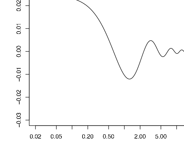
We observe that the kernel is nonlocal, typically varying with the Hubble time scale . Thus the bulk interaction contains a memory. Consequently a local approximation would be possible only if the bound mode varied typically with a time scale larger than the Hubble time.
During inflation, the Hubble radius of the universe remains fairly constant, whereas the physical wavelength of a mode increases exponentially due to the expansion. Early during inflation a mode of a given wave number is initially subhorizon so that . As the universe expands, the mode crosses the horizon to become superhorizon. Whereas modes oscillate at subhorizon scales, they become frozen in after they exit the Hubble horizon. An observer is sensitive to the superhorizon modes on the brane which are the relevant modes to present cosmological observations and constitute the “initial conditions” of the universe at the end of inflation. In that sense we will consider mostly the superhorizon modes, or late-time asymptotics of the modes:
| (121) |
The evolution of the modes at superhorizon scales taking into account the bulk interaction through the integral kernel is nonlocal. Consequently the evolution (and the possible dissipation) of superhorizon modes depends on their past evolution at subhorizon scales through the interaction of the subhorizon modes with the bulk. At superhorizon scales the bare frequency of the bound mode is imaginary
| (122) |
The bare bound mode coefficient excluding the interaction with the bulk is a superposition of a growing mode and a decreasing mode
| (123) | |||||
| (124) |
at superhorizon scales and in the WKB approximation. Since we have rescaled the fields in (85) by the factor , the true bound mode is actually a superposition of a constant mode and a decreasing mode. The bare solutions (123) correspond also to the superhorizon asymptotics of the four dimensional solution given by the Hankel function in the limit of a pure de Sitter four dimensional geometry,
| (125) | |||||
| (126) |
where is the conformal proper time and . The decreasing mode is unobservable and has little cosmological interest for the formation of the large scale structures in the universe. In the following we consider only the dominant solution composed of the growing mode.
We look now for the growing mode of the dressed bound state coefficient with the interaction with the bulk taken into account by using the superhorizon Ansatz
| (127) |
where
| (128) |
Since the bulk interaction kernel is nonlocal, we should take care when inserting this superhorizon Ansatz into the integral kernel in eqn. (116) because the rigorous complete integration should take into account the contribution of the subhorizon regime, where the mode has a form different from the superhorizon Anstaz (127). However, we conjecture that, when observing the dressed superhorizon solution today, the integrated effects of the subhorizon modes in the brane-bulk interaction are subdominant compared to the contribution of the superhorizon modes. This is because the amplitude of subhorizon modes is suppressed compared to the amplitude of superhorizon modes. The choice of the Ansatz (127) at any time for solving the integro-differential equation (116) for the bound state is equivalent to smooth the weak amplitude subhorizon oscillations of the complete mode solution. In that sense we consider the superhorizon Ansatz (127) sufficient to solve the integro-differential equation and compute the order of magnitude of the dissipation rate of the bound state at superhorizon scales.
We now proceed to compute the attenuation factor of the growing bound mode in the regime . In this regime the curvature radius of the extra dimension is much larger than the Hubble radius so that the dissipation rate of the bound state into the extra dimension is expected to reach its maximal value. As we discussed in section 6.1, the plateau potential is a suitable approximation in this regime for the study of the brane-bulk interaction. The height of the plateau potential is then and the dressed bound mode coefficient evolves at superhorizon scales according to the equation
| (129) |
where is the bulk interaction kernel taken in the superhorizon limit, eqn. (118).
Inserting the Ansatz (127) into (129) yields the algebraic equation
| (130) |
which to linear order in becomes
| (131) |
such that
| (132) |
The minus sign in induces attenuation of the growing mode. The plateau potential approximation has the advantage of eliminating the processes of diffraction or reflection in the bulk by smoothing the bulk inhomogeneity, keeping only the dissipative processes due to the extra dimension. Even if the bound state did not dissipate at subhorizon scales and had only its frequency shifted, the bound mode would be observed to dissipate classically in the extra dimension at superhorizon scales as
| (133) |
where is the bare growing mode. The dissipation rate of the bound state at superhorizon scales is given by
| (134) |
The emitted bulk gravitons oscillates at all times because their frequency remains above the plateau of the potential. We may also express the attenuation factor in terms of the four dimensional slow-roll inflation parameter , characterizing the adiabaticity of the expansion of the universe, and the number of e-folds as
| (135) |
The graviton bound state decays nonlocally and quadratically in the slow-roll factor. The dissipation of the zero mode of the graviton during inflation is thus subdominant compared to the dissipation of the inflaton perturbation (section 4).
7 Scalar perturbations in the approximate background: adiabatic perfect fluid on the brane
In this section we study the evolution of scalar metric perturbations in the approximate background geometry (79) accurate near the brane. These perturbations couple to the adiabatic perturbations of a perfect fluid on the brane. They are all described by the single master field as previously discussed in section 3. We take the Fourier transform in the three spatial transverse directions because of the homogeneity and the isotropy, and separately evolve each Fourier mode. In the approximate background geometry (79) near the brane, the equation of motion (38) of the master field in the interval is:
| (136) | |||
| (137) |
where is the transverse momentum. Similarly to the tensor case in section 6, we reduce the equation of motion (136), rescaling
| (138) |
to the equation
| (139) | |||
| (140) |
which contains terms dependent on representing the inhomogeneity of the bulk. The equation of motion is not separable yet. However, as in section 6 for the tensor case when we introduced the plateau potential, we again simpliplify the dependence on retaining only the leading behavior of the coefficients in about . We set
| (141) |
reducing (139) to
| (142) |
where
| (143) | |||||
| (144) |
The bulk curvature is contained in and the intrinsic brane curvature is contained in . We highlight the “wrong” sign in the potential for the scalar perturbations since . The brane behaves as a repulsive potential for the scalar perturbations so that there is no scalar gravitational bound state near the brane as long as there is no coupling to matter on the brane.
The case of a perfect fluid on the brane (with equation of state ) gives rise to some difficulties in computing the evolution of perturbations because the expansion of the brane is no longer adiabatic. is not small except when the fluid is subdominant compared to the brane tension (cosmological constant). Here we explore the damping of the fluid perturbation on subhorizon scales because in this regime the adiabatic approximation of the expansion is valid. At subhorizon scales the geometry of the brane appears quasi-Minkowskian.
The boundary conditions (39) linking the master field to the fluid perturbations on the brane become in the approximate background geometry (79) near the brane
| (145) | |||||
| (146) | |||||
| (148) | |||||
It is possible to simplify the boundary conditions (145) for the scalar metric perturbations by expressing them in terms of the gauge-independent matter perturbation . One obtains the following boundary condition
| (149) |
which, in terms of the rescaled master field (138), becomes
| (150) |
where is given in (143).
The equation of motion for the matter perturbations on the brane can also be derived from the boundary conditions (145) by imposing an equation of state on the matter perturbations. We consider adiabatic matter perturbations with
| (151) |
where the sound speed of the fluid is . One obtains the equation of motion for the matter perturbation , similar to the equation obtained in [21],
| (152) | |||||
| (153) |
where according to the braneworld dynamics [4],[6]
| (154) | |||||
| (155) | |||||
| (156) |
The equation of state of the fluid on the brane is . We may also rescale the brane degree of freedom as to obtain an oscillator equation. Therefore the equations coupling the brane scalar perturbations to the bulk scalar perturbations may be summarized in the generic form
| (157) | |||||
| (158) | |||||
| (159) |
where and are given in (144) and
| (161) | |||||
| (162) | |||||
| (163) |
The immediate observation is the absence of time derivative couplings for the brane-bulk system in (159). Consequently the dissipation of the brane fluid into the bulk can only be nonlocal despite the perfect fluid being local (i.e. truly localized on the brane). Say otherwise, no local friction term such as can appear in the effective equation on the brane, this means that the dissipation of the brane fluid contains a memory or a time delay. The nonlocal brane-bulk interaction comes from the curvature effects.
The underlying physics can be illustrated using the following mechanical model. Consider a string coupled to a harmonic oscillator at the boundary with two springs as indicated in Fig. 6.
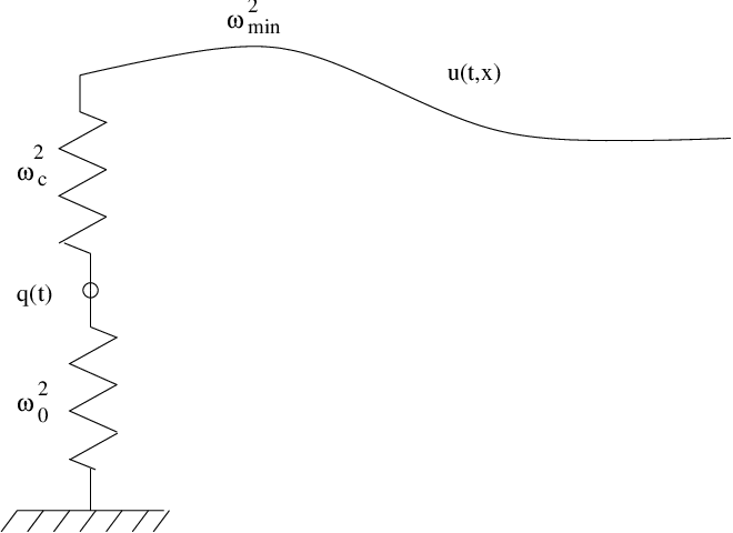
The equations of this model are similar to those obtained for the scalar braneworld perturbations
| (164) | |||||
| (165) | |||||
| (166) |
where is the string tension expressed as a frequency, and and are the spring constants of the two springs expressed as frequencies squared. A toy model very similar to this mechanical system was considered in [27]. The intermediate spring between the mass and the string plays the role of a buffer. In the absence of the buffer the coupling with the string would bring a first derivative local term (friction term) in the effective equation for the harmonic oscillator, indicating a local dissipation of the oscillator down the string.
With no uniform restoring force on the string, the equations would be
| (167) | |||||
| (168) | |||||
| (169) |
where is a forcing term. For coefficients not depending on time, the ansätze and give
| (170) |
which may be rewritten as
| (171) |
where
| (172) | |||||
| (173) | |||||
| (174) |
and Consequently, eqn. (171) becomes
| (175) |
In the limiting case where we may approximate
| (176) |
so that eqn. (175) may be approximated as
| (177) |
We next consider the wave equation for the string including a restoring term, so that there is a minimum frequency for the propagating modes. One has
| (178) |
In this case the kernel is modified to become
| (179) |
When is not too large, , there is an isolated pole at where
| (180) |
and a branch cut on the real axis extending from to To obtain a causal kernel, we must take a contour passing above the branch cut on the real axis. For where the kernel has support, we evaluate the contour by deforming it so that there are two contributions (see Fig. 7(a)). The first term originates from the contour encircling the pole in the clockwise sense
| (181) |
The second originates from the contour encircling the branch cut in the clockwise sense as indicated in Fig.7(a).
| (182) |

As approaches , the pole on the lower half-plane approaches . There is a second pole at the mirror image . However, this pole lies on the other Riemann sheet hidden beyond the branch cut. When exceeds , these two poles collide and scatter at right angles so that they lie on the real line on the branch cut (or just below after the deformation in Fig. 7(b)). We can make both these poles disappear by deforming the branch cut downward as indicated in fig. 7(c). The branch cut has been pushed all the way to negative infinity. Now the kernel integral may be expressed as
| (183) |
where the contours and are indicated in 7(c). We may rewrite this as
| (185) | |||||
In fact this expression also holds for . At large times the kernel (185) behaves asymptotically as
| (186) |
We also compute the kernel in Fourier space. With the forcing term the oscillator equation is
| (187) | |||||
| (188) |
The time average of the power transmitted to the oscillator (which is a measure of the dissipation) is
| (189) | |||||
| (190) | |||||
| (191) |
If the kernel has no imaginary part, the system exchanges energy but does not dissipate since the average power vanishes. For the imaginary part of the kernel vanishes. From we deduce the average dissipated power
| (192) |
The dissipated power is zero when . One can understand qualitatively how the behavior changes as is varied. The string may be regarded as a high pass filter with threshold . Only radiation of higher frequency can escape down the string to infinity, thus leading to a net flux of power away from the oscillator. At lower frequencies the string is excited around the oscillator but in a localized way with the amplitude decaying exponentially with distance from the oscillator since the extra momentum from the bulk wave equation becomes imaginary. In this case there is no dissipation in the long term because the string vibrates in phase with the oscillator. Of course the coupling shifts the frequency of the oscillator because the string adds both inertia and restoring force to the oscillator.
For the brane-bulk system, the threshold is given by
| (193) |
where , have been computed in (144). For a weak coupling to the bulk (), the frequency of the brane degree of freedom is only slightly displaced from its bare frequency given in eqn. (161). At subhorizon scales (),
| (194) |
because . Therefore the dissipated power is exactly zero. In the adiabatic approximation, valid on subhorizon scales, the fluid cannot dissipate into the bulk because the natural frequency of the bulk mode at the same wavenumber is too high to have a resonance.
8 Discussion and conclusions
In this paper we presented analytic approaches to estimate the order of magnitude of the dissipative effects in braneworld cosmology affecting the evolution of both scalar and tensor perturbations on the brane. Because of the non-uniform expansion of the brane, the degrees of freedom on the brane interact with the bulk gravitons, possibly leading to dissipation from the four dimensional perspective. These effects are encoded in the bulk retarded propagator. From the dressed brane propagator, obtained by resumming the bulk backreaction effects at all order in the brane-bulk coupling, we may extract the effective dissipation rate of certain brane degrees of freedom. We assumed an adiabatic expansion on the brane () in order to apply our methods.
Our analytic results provide more intuition on the previous numerical simulations regarding braneworld slow-roll inflation [23]. For the scalar perturbations with a slow-roll inflaton field on the brane we obtained, without any other approximation, the local dissipation rate of the inflaton perturbation due to its interaction with the bulk gravitons, , which is linear in the slow-roll factor. This is our main result and agrees with the numerical results obtained by Koyama & al. in [23]. In the high-energy limit of braneworld inflation () the correction to standard inflation due to the coupling to bulk metric perturbations is found to be linear in the slow-roll factor as well. Moreover the dependence on of the dissipation rate correctly fits the behaviour of the slow-roll correction plotted in [23].
For the tensor perturbations we encounter purely nonlocal brane-bulk interaction, that is why we simplified the backgound geometry: we explicitely neglected the nonlocal processes on the brane due to backscattering of bulk gravitons in curved assuming that the dissipation is the dominant effect on the brane by considering the near-brane limit of the bulk geometry (plateau potential). This approximation is well legitimized in the high-energy regime of braneworld inflation () because the bulk curvature becomes negligeable compared to the acceleration of the brane. We were able in this way to compute the slow-roll correction to tensor perturbations due to the coupling of the zero mode with the continuum of bulk gravitons. We found a small attenuation of the growing mode of the graviton bound state at superhorizon scales and at high energy due to its interaction with the bulk modes and we obtained that this correction is quadratic in the slow-roll factor, . This is a new result. The inflaton field perturbation thus decays at a larger rate , linear in the adiabatic slow-roll parameter, than the decay rate the graviton bound state , quadratic in the slow-roll parameter at high-energy. This difference is the consequence of the locality of the interaction between the inflaton and the bulk modes as opposed to the nonlocal interaction between the graviton bound mode and the bulk modes. We also found that an adiabatic perfect fluid on the brane does not dissipate into the extra dimension at subhorizon scales because the minimum frequency of the bulk modes at the same wavenumber as the fluid is too high to have a resonance. We encounter some difficulties in applying analytic methods for the perfect fluid at superhorizon scales because at such scales the expansion of the brane is no longer adiabatic, at least when the fluid dominates the tension of the brane.
It would be interesting to go beyond the plateau potential approximation
by taking into account the inhomogeneity of the bulk and the diffraction of the
gravitons by the bulk which lead to nonlocal effects on the brane. The
nonlocality is encoded in the bulk propagator and depends strongly on
the bulk curvature. In that sense the exact expression of the
propagator is necessary to compute the nonlocal effects. The
curved geometry of the bulk also requires the existence of metastable gravitons or
quasi-bound states on the brane even if the brane is static as it was found by Seahra [28]. We
could compare the flux of the tunneling bulk gravitons with the flux of the
quasi-bound states. This will be the object of a future publication.
Acknowledgments
I would like to thank Martin Bucher, Carla Carvalho, Christos Charmousis and Renaud Parentani for useful discussions.
References
- [1] L. Randall and R. Sundrum, “An Alternative to Compactification," Phys. Rev. Lett. 83, 4690 (1999); L. Randall and R. Sundrum, “A Large Mass Hierarchy From a Small Extra Dimension,” Phys. Rev. Lett. 83, 3370 (1999).
- [2] J. Garriga and T. Tanaka, “Gravity in the Randall-Sundrum Brane World,” Phys. Rev. Lett. 84, 2778 (2000).
- [3] D. J. Kapner, T. S. Cook, E. G. Adelberger, J. H. Gundlach, B. R. Heckel, C. D. Hoyle and H. E. Swanson, “Tests of the Gravitational Inverse-Square Law below the Dark-Energy length scale,” Phys. Rev. Lett. 98:021101 (2007).
- [4] P. Binétruy, C. Deffayet, U. Ellwanger and D. Langlois, “Brane Cosmological Evolution in a Bulk With Cosmological Constant,” Phys. Lett. B477, 285 (2000); P. Binétruy, C. Deffayet and D. Langlois, “Nonconventional Cosmology From a Brane Universe,” Nucl. Phys. B565, 269 (2000); P. Bowcock, C. Charmousis and R. Gregory, “General Brane Cosmologies and their Global Space-Time Structure,” Class. Quant. Grav. 17, 4745 (2000); T. Shiromizu, K. Maeda and M. Sasaki, “The Einstein Equations on the 3-Brane World,” Phys. Rev. D 62, 024012 (2000).
- [5] J. Garriga and M. Sasaki, "Brane-World Creation and Black Holes," Phys. Rev. D62:043523 (2000); D. Langlois, R. Maartens and D. Wands , “Gravitational Waves from Inflation on the Brane,” Phys. Lett. B489, 259 (2000); A. V. Frolov and L. Kofman, “Gravitational Waves from Brane World Inflation,” hep-th/0209133.
- [6] C. Deffayet, “On Brane World Cosmological Perturbations,” Phys. Rev. D66, 103504 (2002); C. Deffayet, “Note on the Well-Posedness of Scalar Brane World Cosmological Perturbations,” Phys. Rev. D71, 023520 (2005).
- [7] D. Langlois, “Brane Cosmological Perturbations,” Phys. Rev. D62, 126012 (2000); R. Easther, D. Langlois, R. Maartens and D. Wands, “Evolution of Gravitational Waves in Randall-Sundrum Cosmology,” JCAP 0310, 014 (2003); A. Riazuelo, F. Vernizzi, D. Steer and R. Durrer, “Gauge Invariant Cosmological Perturbation Theory for Braneworlds,” hep-th/0205220; D. Langlois, L. Sorbo, M. Rodriguez-Martinez, “Cosmology of a Brane Radiating Gravitons Into the Extra Dimension,” Phys. Rev. Lett. 89, 171301 (2002); D. Langlois, R. Maartens, M. Sasaki, D. Wands, “Large Scale Cosmological Perturbations on the Brane,” Phys. Rev. D63, 084009 (2001); R. A. Battye, C. van de Bruck and A. Mennim, “Cosmological Tensor Perturbations in the Randall-Sundrum Model: Evolution in the Near-Brane Limit,” Phys. Rev. D69, 064040 (2004).
- [8] S. Mukohyama, “Gauge Invariant Gravitational Perturbations of Maximally Symmetric Spacetimes,” Phys. Rev. D62, 084015 (2000); S. Mukohyama, “Perturbation of Junction Condition and Doubly Gauge Invariant Variables,” Class. Quant. Grav. 17, 4777 (2000); S. Mukohyama, “Integro-differential Equation for Brane World Cosmological Perturbations,” Phys. Rev. D64:064006 (2001) (Erratum-ibid. D66, 049902 (2002)); S. Mukohyama, “Doubly Covariant Action Principle of Singular Hypersurfaces in General Relativity and Scalar-Tensor Theories,” Phys. Rev. D65, 024028 (2002); S. Mukohyama, “Doubly Covariant Gauge Invariant Formalism of Braneworld Cosmological Perturbations,” hep-th/0202100; S. Mukohyama, “Nonlocality as an Essential Feature of Brane Worlds,” Prog. Theor. Phys. Suppl. 148, 121 (2003).
- [9] H. Kodama, A. Ishibashi and O. Seto, “Brane World Cosmology: Gauge-Invariant Formalism for Perturbation,” Phys. Rev. D62, 064022 (2000).
- [10] H. A. Bridgman, K. A. Malik and D. Wands, “Cosmological Perturbations in the Bulk and on the Brane,” Phys. Rev. D65, 043502 (2002).
- [11] D. S. Gorbunov, V. A. Rubakov and S. M. Sibiryakov, “Gravity Waves From Inflating Brane or Mirrors Moving in AdS5,” JHEP 0110, 015 (2001); T. Kobayashi, H. Kudoh and T. Tanaka, “ Primordial Gravitational Waves in Inflationary Brane World,” Phys. Rev. D68:044025 (2003).
- [12] N. Deruelle, “Cosmological Perturbations of an Expanding Brane in an Anti-de Sitter Bulk: A Short Review,” Astrophys. Space Sci. 283:619-626 (2003).
- [13] K. Koyama, “Late Time Behaviour of Cosmological Perturbations in a Single-Brane Model,” JCAP0409,010 (2004); K. Koyama, D. Langlois, R. Maartens and D. Wands, “Scalar Perturbations from Brane-World Inflation,” JCAP0411,002 (2004).
- [14] T. Hiramatsu, K. Koyama and A. Taruya, “Evolution of gravitational waves from inflationary brane world : numerical study of high-energy effects,” Phys.Lett.B578:269-275 (2004).
- [15] T. Hiramatsu, K. Koyama and A. Taruya, “Evolution of gravitational waves in the high-energy regime of brane-world cosmology,” Phys.Lett.B609:133-142 (2005).
- [16] T. Hiramatsu and K. Koyama , “ Numerical Study of Curvature Perturbations in a Brane-World Inflation at High-Energies,” JCAP 0612:009 (2006).
- [17] T. Hiramatsu, “High-energy effects on the spectrum of inflationary gravitational wave background in braneworld cosmology,” Phys.Rev.D73:084008 (2006).
- [18] T. Kobayashi and T. Tanaka, “Quantum-mechanical generation of gravitational waves in braneworld,” Phys.Rev.D71:124028 (2005).
- [19] T. Kobayashi, “Initial Kaluza-Klein Fluctuations and Inflationary Gravitational Waves in Braneworld Cosmology,” Phys. Rev. D73:124031 (2006).
- [20] S. S. Seahra, “Gravitational Waves and Cosmological Braneworlds: A Characteristic Evolution Scheme,” Phys. Rev. D74:044010 (2006).
- [21] A. Cardoso, T. Hiramatsu, K. Koyama and S. S. Seahra, “Scalar Perturbations in Braneworld Cosmology,” arXiv:0705.1685[astro-ph].
- [22] K. Koyama, A. Mennim, V. A. Rubakov, D. Wands and T. Hiramatsu, “Primordial Perturbations from Slow-roll Inflation on a Brane,” JCAP 0704:001 (2007).
- [23] K. Koyama, A. Mennim and D. Wands, “Brane-world inflation: Slow-roll corrections to the spectral index,” Phys.Rev.D77:021501 (2008).
- [24] G. D. Starkman, D. Stojkovic and M. Trodden, “Homogeneity, Flatness and ’Large’ Extra Dimensions,” Phys.Rev.Lett.87:231303 (2001); G. D. Starkman, D. Stojkovic and M. Trodden, “Large Extra Dimensions and Cosmological Problems,” Phys.Rev.D63:103511 (2001).
- [25] M. Bucher, “A Brane World Universe from Colliding Bubbles,” Phys.Lett.B530:1-9 (2002).
- [26] P. Binetruy, M. Bucher and C. Carvalho, “Models for the Brane Bulk Interaction: Toward Understanding Brane World Cosmological Perturbations,” Phys. Rev. D70:043509 (2004); M. Bucher and C. Carvalho, “ Linearized Israel Matching Conditions for Cosmological Perturbations in a Moving Brane Background,” Phys. Rev. D71:083511 (2005).
- [27] K. Koyama, A. Mennim and D. Wands, “Coupled boundary and bulk fields in Anti-de Sitter spacetime,” Phys.Rev.D72:064001 (2005); A. Cardoso, K. Koyama, A. Mennim, S. S. Seahra and D. Wands, “Coupled Bulk and Brane Fields about a de Sitter Brane,” Phys. Rev. D75:084002 (2007).
- [28] S. S. Seahra, “Ringing the Randall-Sundrum braneworld:Metastable gravity wave bound states,” Phys.Rev.D72:066002 (2005); S. S. Seahra, “Metastable Massive Gravitons from an Infinite Extra Dimension,” Int. J. Mod. Phys. D14:2279-2284 (2005).