Inhomogeneous Bulk Viscous Fluid Universe with Electromagnetic Field and Variable
-Term
Anirudh Pradhan 11 1 Corresponding author, Vandana Rai 2, Kanti Jotania3
1 Department of Mathematics, Hindu Post-graduate College, Zamania-232 331, Ghazipur, India
E-mail : pradhan@iucaa.ernet.in
2Department of Mathematics, Post-graduate College, Ghazipur-233 001, India
E-mail : vandana_rai005@yahoo.co.in
3Department of Physics, Faculty of Science, The M. S. University of Baroda, Vadodara-390 002, India
E-mail : kanti@iucaa.ernet.in
Keywords : cosmology, variable cosmological term, electromagnetic field, inhomogeneous universe
PACS number: 98.80.Jk, 98.80.-k
Abstract
Cylindrically symmetric inhomogeneous cosmological model for bulk viscous fluid distribution with electromagnetic field is obtained. The source of the magnetic field is due to an electric current produced along the z-axis. is the non-vanishing component of electromagnetic field tensor. To get the deterministic solution, it has been assumed that the expansion in the model is proportional to the shear . The values of cosmological constant for these models are found to be small and positive at late time which are consistent with the results from recent supernovae Ia observations. Physical and geometric aspects of the models are also discussed in presence and absence of magnetic field.
1 Introduction
Inhomogeneous cosmological models play an important role in understanding some essential features of the universe such as the formation of galaxies during the early stages of evolution and process of homogenization. The early attempts at the construction of such models have been done by Tolman [1] and Bondi [2] who considered spherically symmetric models. Inhomogeneous plane-symmetric models were considered by Taub [3, 4] and later by Tomimura [5], Szekeres [6], Collins and Szafron [7], Szafron and Collins [8]. Recently, Senovilla [9] obtained a new class of exact solutions of Einstein’s equations without big bang singularity, representing a cylindrically symmetric, inhomogeneous cosmological model filled with perfect fluid which is smooth and regular everywhere satisfying energy and causality conditions. Later, Ruiz and Senovilla [10] have examined a fairly large class of singularity free models through a comprehensive study of general cylindrically symmetric metric with separable function of and as metric coefficients. Dadhich et al. [11] have established a link between the FRW model and the singularity free family by deducing the latter through a natural and simple in-homogenization and anisotropization of the former. Also, Patel et al. [12] presented a general class of inhomogeneous cosmological models filled with non-thermalized perfect fluid by assuming that the background space-time admits two space-like commuting Killing vectors and has separable metric coefficients. Singh, Mehta and Gupta [13] obtained inhomogeneous cosmological models of perfect fluid distribution with electro-magnetic field. Recently, Pradhan et al. [14] have investigated plane-symmetric inhomogeneous cosmological models in various contexts. Cylindrically symmetric space-time play an important role in the study of the universe on a scale in which anisotropy and inhomogeneity are not ignored. Roy and Singh [15], Bali and Tyagi [16, 17], Chakrabarty et al. [18] and Pradhan et al. [19] have investigated cylindrically symmetric inhomogeneous cosmological models in presence of electromagnetic field.
The occurrence of magnetic field on galactic scale is well-established fact today, and their importance for a variety of astrophysical phenomena is generally acknowledged as pointed out by Zeldovich et al. [20]. Also Harrison [21] has suggested that magnetic field could have a cosmological origin. As a natural consequences, we should include magnetic fields in the energy-momentum tensor of the early universe. The choice of anisotropic cosmological models in Einstein system of field equations leads to the cosmological models more general than Robertson-Walker model [22]. The presence of primordial magnetic field in the early stages of the evolution of the universe has been discussed by several authors [23][32]. Strong magnetic field can be created due to adiabatic compression in clusters of galaxies. Large-scale magnetic field gives rise to anisotropies in the universe. The anisotropic pressure created by the magnetic fields dominates the evolution of the shear anisotropy and it decays slower than the case when the pressure was isotropic [33, 34]. Such fields can be generated at the end of an inflationary epoch [35][39]. Anisotropic magnetic field models have significant contribution in the evolution of galaxies and stellar objects. Bali and Ali [40] obtained a magnetized cylindrically symmetric universe with an electrically neutral perfect fluid as the source of matter. Chakrabarty et al. [18] and Pradhan et al. [41] have investigated magnetized viscous fluid cosmological models in various contexts.
There are significant observational evidence for the detection of Einstein’s cosmological constant,
or a component of material content of the universe that varies slowly with time and space
to act like . Some of the recent discussions on the cosmological constant “problem” and on
cosmology with a time-varying cosmological constant by Ratra and Peebles [42], and Sahni and
Starobinsky [43] point out that in the absence of any interaction with matter or radiation,
the cosmological constant remains a “constant”. However, in the presence of interactions with matter
or radiation, a solution of Einstein equations and the assumed equation of covariant conservation
of stress-energy with a time-varying can be found. This entails that energy has to be conserved
by a decrease in the energy density of the vacuum component followed by a corresponding increase in the
energy density of matter or radiation (see also Carroll, Press and Turner [44], Peebles [45],
Padmanabhan [46]). There is a plethora of astrophysical evidence today, from supernovae measurements
(Perlmutter et al. [47], Riess et al. [48], Garnavich et al. [49], Schmidt et al.
[50], Blakeslee et al. [51], Astier et al. [52]), the spectrum of fluctuations in
the Cosmic Microwave Background (CMB) [53], baryon oscillations [54] and other astrophysical
data, indicating that the expansion of the universe is currently accelerating. The energy budget of the
universe seems to be dominated at the present epoch by a mysterious dark energy component, but the precise
nature of this energy is still unknown. Many theoretical models provide possible explanations for the dark
energy, ranging from a cosmological term [55] to super-horizon perturbations [56] and
time-varying quintessence scenarios [57]. These recent observations strongly favour a significant
and a positive value of with magnitude .
In Ref. [48], Riess et al. have recently presented an analysis of 156 SNe including a few at
from the Hubble Space Telescope (HST) “GOOD ACS” Treasury survey. They conclude to the
evidence for present acceleration . Observations (Knop et al. [58];
Riess et al., [48]) of Type Ia Supernovae (SNe) allow us to probe the expansion history of the
universe leading to the conclusion that the expansion of the universe is accelerating.
Most studies in cosmology involve a perfect fluid. Large entropy per baryon and the remarkable degree of isotropy of the cosmic microwave background radiation, suggest that we should analyze dissipative effects in cosmology. Further, there are several processes which are expected to give rise to viscous effect. These are the decoupling of neutrinos during the radiation era and the recombination era [59], decay of massive super string modes into massless modes [60], gravitational string production [61, 62] and particle creation effect in grand unification era [63]. It is known that the introduction of bulk viscosity can avoid the big bang singularity. Thus, we should consider the presence of a material distribution other than a perfect fluid to have realistic cosmological models (see Grøn [64] for a review on cosmological models with bulk viscosity). A uniform cosmological model filled with fluid which possesses pressure and second (bulk) viscosity was developed by Murphy [65]. The solutions that he found exhibit an interesting feature that the big bang type singularity appears in the infinite past.
Recently, Pradhan et al. [66] have obtained inhomogeneous perfect fluid universe with electromagnetic field. Motivated by the situation discussed above, in this paper, we have obtained a new cylindrically symmetric inhomogeneous cosmological model for bulk viscous fluid distribution in presence and absence of electromagnetic field. The coefficient of bulk viscosity is assumed to be a power function of mass density. This work generalize the previous work of Pradhan et al. [66]. Some physical and geometric behaviour of the models in presence and absence of magnetic field are also discussed. This paper is organized as follows. The metric and the field equations are laid down in Section 2. In Section 3, we deal with the solutions of the field equations in presence of bulk viscous fluid with electromagnetic field and variable cosmological term. We have also described the physical and geometric aspects of the models. In Section 4, we obtain the solutions of the field equations in absence of the magnetic field. Finally in Section 5 concluding remarks are given.
2 The Metric and Field Equations
We consider the metric in the form
| (1) |
where is the function of alone and and are functions of and . The energy momentum tensor is taken as has the form
| (2) |
where is the electromagnetic field given by Lichnerowicz [67]
| (3) |
and
| (4) |
Here , , and are the energy density, isotropic pressure, effective pressure and bulk viscous coefficient respectively and is the fluid four-velocity vector satisfying the condition
| (5) |
is the magnetic permeability and , the magnetic flux vector defined by
| (6) |
where the dual electromagnetic field tensor is defined by Synge [68]
| (7) |
Here is the electromagnetic field tensor and is the Levi-Civita
tensor density.
The co-ordinates are considered to be comoving so that = = = and
. If we consider that the current flows along the -axis, then is the only
non-vanishing component of . The Maxwell’s equations
| (8) |
| (9) |
require that is the function of -alone. We assume that the magnetic permeability is the
functions of and both. Here the semicolon represents a covariant differentiation.
The Einstein’s field equations (in gravitational units ) read
| (10) |
for the line-element (1) lead to the following system of equations:
| (11) |
| (12) |
| (13) |
| (14) |
| (15) |
where the sub indices and in A, B, C and elsewhere denote ordinary differentiation with respect to and respectively.
3 Solution of the Field Equations
Equations (11)-(15) are five independent equations in six unknowns , , ,
, and . For the complete determinacy of the system, we need one extra condition.
The research on exact solutions is based on some physically reasonable restrictions used to simplify
the Einstein equations.
To get determinate solution we assume that the expansion in the model is proportional to the
shear . This condition leads to
| (16) |
where is a constant. From Eqs. (11)-(13), we have
| (17) |
and
| (18) |
We also assume that
| (19) |
Using Eqs. (16) and (17) in (15) and (17) lead to
| (20) |
| (21) |
| (22) |
Equation (20) leads to
| (23) |
where and is the constant of integration. From Eqs. (21) and (23), we have
| (24) |
where
Equation (22) leads to
| (25) |
where is an integrating constant. Equation (24) leads to
| (26) |
where and , are integrating constants. Hence from (23) and (26), we have
| (27) |
Therefore we obtain
| (28) |
| (29) |
| (30) |
where , being a constant of integration.
After using suitable transformation of the co-ordinates, the model (1) reduces to the form
| (31) |
where , , , .
The expressions for effective pressure and density for the model (31) are given by
| (32) |
| (33) |
For the specification of , we assume that the fluid obeys an equation of state of the form
| (34) |
where is a constant. Thus, given we can solve for the cosmological parameters. In most of the investigation involving bulk viscosity it is assumed to be a simple power function of the energy density [69][73]
| (35) |
where and are constants. For small density, may even be equal to unity as used in Murphy’s
work [65] for simplicity. If , (35) may correspond to a radiative fluid [73].
Near a big bang, is a more appropriate assumption [74] to obtain realistic
models.
| (36) |
where is the scalar of expansion calculated for the flow vector and is given by
| (37) |
where
| (38) |
For simplicity and realistic models of physical importance, we consider the following two cases . On using (35) in (32), we obtain
3.1 Model I: Solution when
When , Eq. (35) reduces to . With the use of Eqs. (33), (34) and (37), Eq. (36) reduces to
| (39) |
Eliminating between (33) and (39), we get
| (40) |
where

3.2 Model II: Solution when
When , Eq. (35) reduces to . With the use of Eqs. (33), (34) and (37), Eq. (36) reduces to
| (41) |
Eliminating between (33) and (41), we get
| (42) |

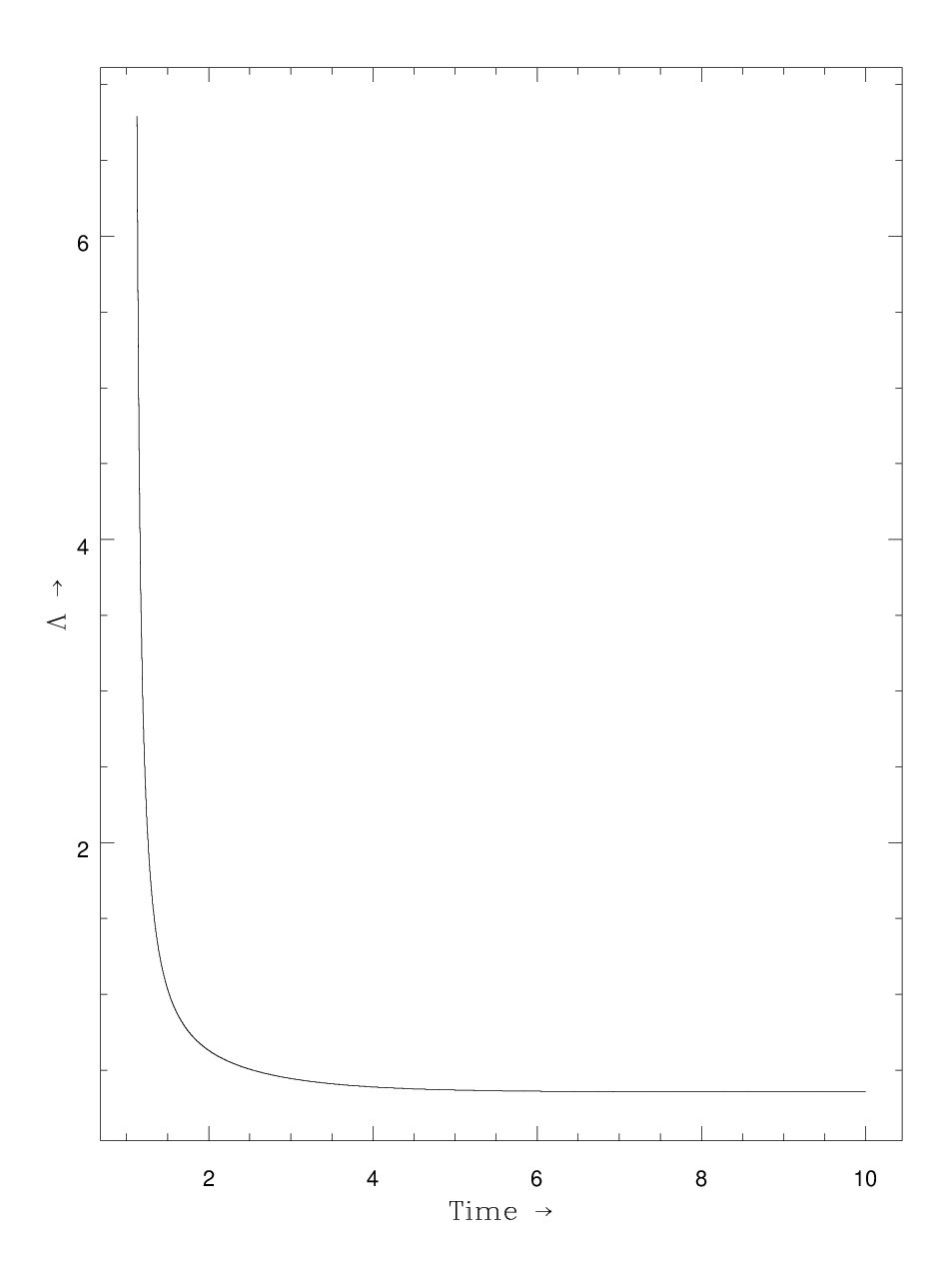
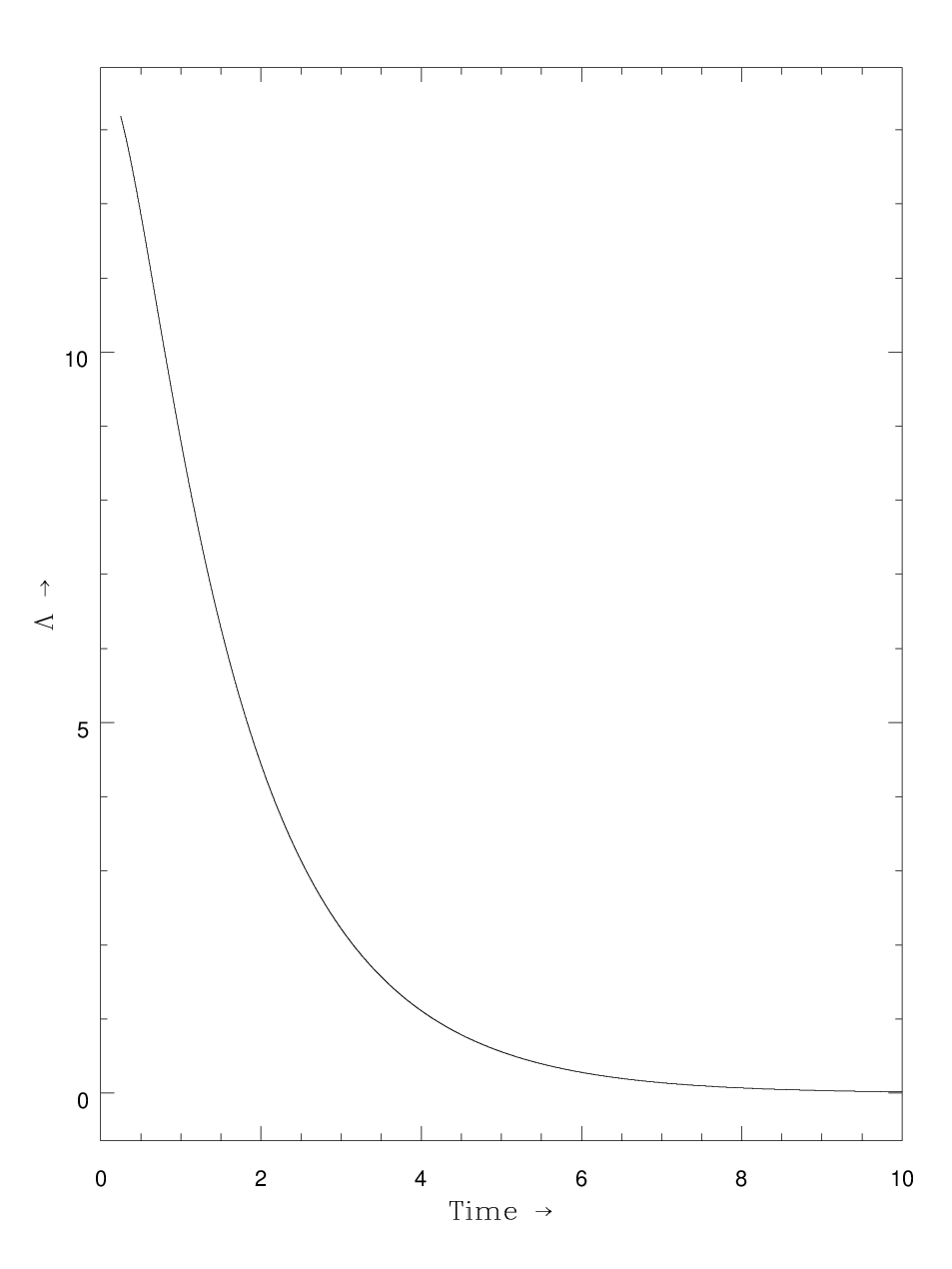
From Eqs. (39) and (41) , we note that is a decreasing function of time
and for all times. This behaviour is clearly depicted in Figures and as a representative
case with appropriate choice of constants of integration and other physical parameters using reasonably
well known situations. Figures and show this physical behaviours of energy density as a decreasing
functions of coordinate time of Model I and II. Here the coordinate time is related to normal time as shown
in Ref.[19]. This also follows for rest part of the paper.
In spite of homogeneity at large scale our universe is inhomogeneous at small scales, so physical
quantities being position dependent are more natural in our observable universe if we do not go
to super high scale. This result shows this kind of physical importance. In recent time the -term
has interested theoreticians and observers for various reasons. The nontrivial role of the vacuum in
the early universe generate a -term that leads to inflationary phase. Observationally, this term
provides an additional parameter to accommodate conflicting data on the values of the Hubble constant, the
deceleration parameter, the density parameter and the age of the universe (for example, see the references
[75, 76]). Assuming that owes its origin to vacuum interactions, as suggested in
particular by Sakharov [77], it follows that it would in general be a function of space and time
coordinates, rather than a strict constant. In a homogeneous universe will be at most time dependent
[78]. In our case this approach can generate that varies both with space and time. In
considering the nature of local massive objects, however, the space dependence of cannot be ignored.
For details discussion, the readers are advised to see the references (Narlikar, Pecker and Vigier
[79], Ray and Ray [80], Tiwari, Ray and Bhadra [81]).
The behaviour of the universe in this model will be determined by the cosmological term ; this term
has the same effect as a uniform mass density , which is constant in space
and time. A positive value of corresponds to a negative effective mass density (repulsion). Hence, we
expect that in the universe with a positive value of , the expansion will
tend to accelerate; whereas in the universe with negative value of , the expansion will slow down, stop
and reverse. From Eqs. (40) and (42), we see that the cosmological term is a decreasing
function of time and it approaches a small positive value at late time. From Figures 2 and 4, we note this behaviour
of cosmological term in both models I and II. Recent cosmological observations suggest the existence
of a positive cosmological constant with the magnitude . These
observations on magnitude and red-shift of type Ia supernova suggest that our universe may be an accelerating
one with induced cosmological density through the cosmological -term. Thus, our model is consistent
with the results of recent observations.
Some Physical and Geometric Features :
The non-vanishing component of electromagnetic field tensor is obtained as
| (43) |
The expressions for the shear scalar , acceleration vector and proper volume for model (31) are given by
| (44) |
| (45) |
| (46) |
From Eqs. (44) and (37), we have
| (47) |
The rotation is identically zero. From set of equations (37), (43) - (47),
the model brings out the following features:
The model starts expanding at and goes on expanding indefinitely when .
The model (31) represents an expanding, shearing and non-rotating universe in which the flow vector is geodetic.
Since = constant, the model does not approach isotropy. As increases
the proper volume also increases. The model is non-accelerating. The physical quantities and
decrease as increases. However, if ,
the process of contraction starts at and at the expansion stops. The electromagnetic
field tensor does not vanish when , and .
4 Solution in Absence of Magnetic Field
In absence of magnetic field the Einstein field equations for metric (1) read as
| (48) |
| (49) |
| (50) |
| (51) |
| (52) |
| (53) |
| (54) |
| (55) |
which on integration gives
| (56) |
where and are constants of integration. Hence from (23) and (56), we have
| (57) |
In this case (17) leads to
| (58) |
Therefore, we have
| (59) |
| (60) |
| (61) |
where is already defined in previous section.
After using suitable transformation of the co-ordinates, the model (1) reduces to the form
| (62) |
where , , , .
The expressions for effective pressure and density for the model (62) are given by
| (63) |
| (64) |
On using (35) in (63), we obtain
| (65) |
where , in this case, is calculated for the flow vector and is given by
| (66) |
where
| (67) |
4.1 Model I: Solution when

Eliminating between (64) and (68), we get
| (69) |
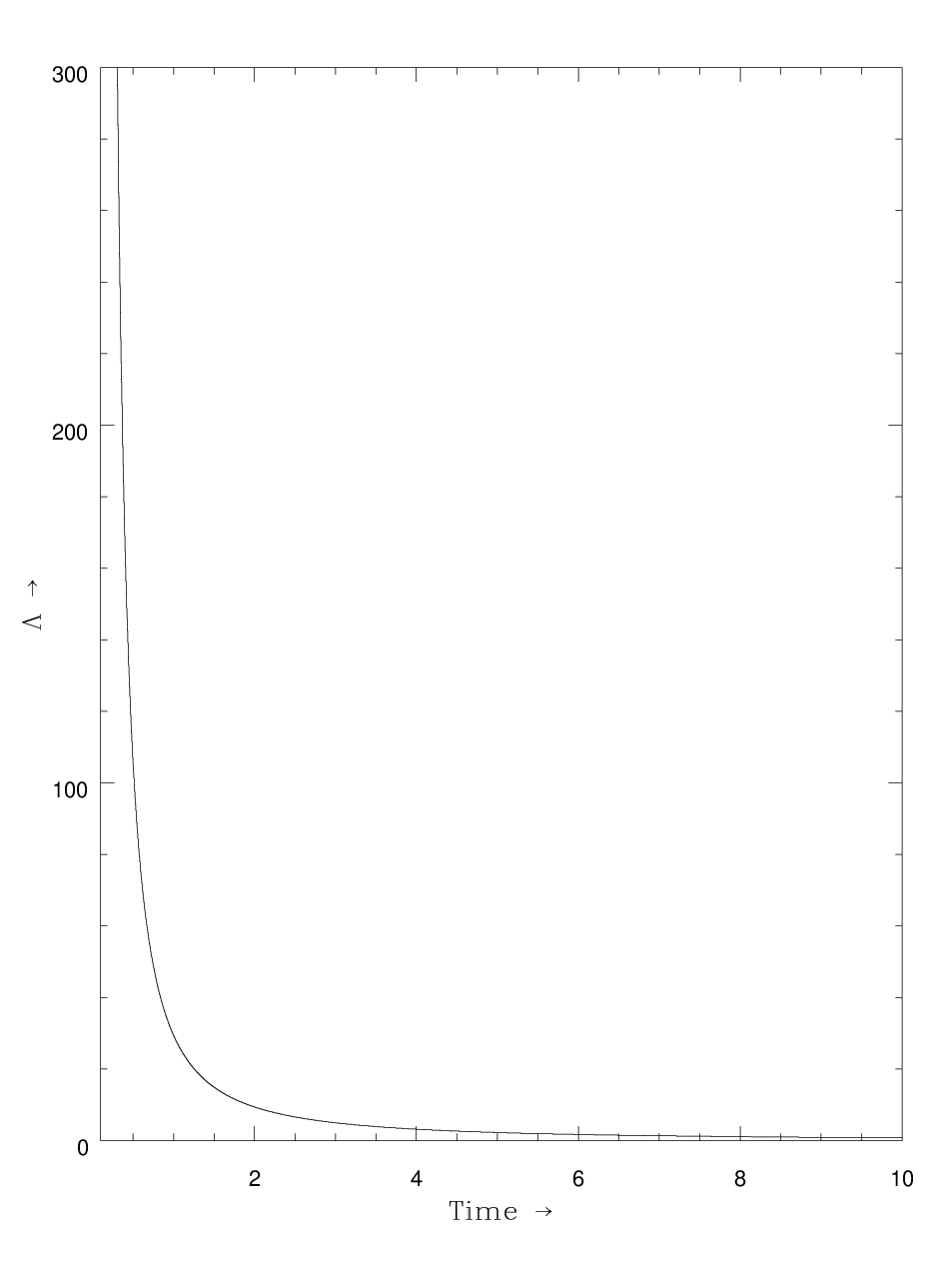
From Eq. (68), we see that is a decreasing function of time and for
all times. Figure shows this behaviour of energy density in Model I.
From Eq. (69), we observe that the cosmological term is a decreasing function of time and it
approaches a small positive value at late time. From Figure , we note this behaviour
of cosmological term in both model I.
4.2 Model II: Solution when

Eliminating between (64) and (70), we get
| (71) |
From Eq. (70) and also from Figure , it seems that in very early stage of universe the energy density
could be negative and may be link with some of the early universe physics which is the domain of quantum cosmology
or early quantum mechanics. So we do not infer any things about energy density. But note that once energy density
is negative in the initial stage even after oscillations it returns back to small negative value at the later stage
of the evolution. Hence the details of macro physics in early universe decides its fate. So we cannot infer from
this model. Similar behaviours is also reflected about the cosmological constant . We do not know for
wide range of parameters this behaviour holds. It may be feasible that Figures may coincide with Figures
and . But it does not seem to be vary generic behaviour of generalized model of section . So we do not
go to any conclusion about its applicability in general. But it seems that magnetic field and bulk viscosity prevent
this kind of unusual behaviours as it is clear from Figures to .
Some Physical and Geometric Features:
The expressions for the shear scalar , acceleration vector and proper volume for model (62) are given by
| (72) |
| (73) |
| (74) |
| (75) |
The rotation is identically zero.
The model in absence of magnetic field starts expanding with a big bang at and it stops expanding at . In absence of magnetic field, the model in general represents an expanding, shearing and non-rotating in which the flow vector is geodetic. Since = constant, the model does not approach isotropy. As increases the proper volume also increases. The model is non-accelerating.
5 Concluding Remarks
We have obtained a new cylindrically symmetric inhomogeneous cosmological model of electro-magnetic
bulk viscous fluid as the source of matter. Generally the model represents expanding, shearing and non-
rotating universe in which the flow vector is geodetic. It is worth mention here that in presence
of magnetic field the model (31) is expanding whereas in absence of magnetic field the model
(62) starts with a big bang singularity. In both models constant
and hence they do not approach isotropy. The models are non-accelerating. In these solutions all
physical quantities depend on at most one space co-ordinate and time.
It is important to note here that both the models (31) and (62) in presence and
absence of magnetic field reduce to homogeneous universe when . This shows that
for , inhomogeneity dies out.
The effect of bulk viscosity is to produce a change in perfect fluid and hence exhibit essential influence
on the character of the solution. The effect is clearly visible on the effective (see details in previous
sections). In Section , we have shown regular well behaviour of energy density, cosmological constant ()
and the expansion of the universe with parameter . The section is a toy investigation to see that the
effect of bulk viscosity plays dynamic role in the evolution equations. We also observe that Murphy’s conclusion
[65] about the absence of a big bang type singularity in the infinite past in models with bulk viscous
fluid, in general, is not true. The results obtained by Myung and Cho [60] also show that, it is, in general,
not valid, since for some cases big bang singularity occurs in finite past.
In presence and absence of magnetic field, the cosmological terms in models are decreasing function of time and approach a small value at late time (with exception in the absence of magnetic field). The values of cosmological “constant” for the models are found to be small and positive, as obtained in recent results from the supernovae observations recently obtained by the High-Z supernovae Ia Team and Supernovae Cosmological Project. Our solutions generalize the solutions recently obtained by Pradhan et al. [66].
Acknowledgments
Authors would like to thank the Inter-University Centre for Astronomy and Astrophysics (IUCAA), Pune, India for providing facility and support where this work was carried out. A. P. and K. J. are visiting associates of IUCAA.
References
- [1] R. C. Tolman, Proc. Nat. Acad. Sci. 20 (1934) 169.
- [2] H. Bondi, Mon. Not. R. Astro. Soc. 107 (1947) 410.
- [3] A. H. Taub, Ann. Math. 53 (1951) 472.
- [4] A. H. Taub, Phy. Rev. 103 (1956) 454.
- [5] N. Tomimura, II Nuovo Cimento B 44 (1978) 372.
- [6] P. Szekeres, Commun. Math. Phys. 41 (1975) 55.
- [7] C. B. Collins and D. A. Szafron, J. Math. Phy. 20 (1979) 2347; J. Math. Phy. 20 (1979b) 2362.
- [8] D. A. Szafron and C. B. Collins, J. Math. Phy. 20 (1979) 2354.
- [9] J. M. M. Senovilla, Phy. Rev. Lett. 64 (1990) 2219.
- [10] E. Ruiz and J. M. M. Senovilla, Phy. Rev. D 45 (1990) 1995.
- [11] N. Dadhich, R. Tikekar and L. K. Patel, Curr. Sci. 65 (1993) 694.
- [12] L. K. Patel, R. Tikekar and N. Dadhich, Pramana-J. Phys. 49 (1993) 213.
- [13] G. Singh, P. Mehta and S. Gupta, Astrophys. Space Sci. 281 (1990) 677.
- [14]
A. Pradhan, V. K. Yadav and N. N. Saste, Int. J. Mod. Phys. D 11 (2002) 857;
A. Pradhan and H. R. Pandey, Int. J. Mod. Phys. D 12 (2003) 941;
A. Pradhan and P. Pandey, Czech. J. Phys. 55 (2005) 749;
A. Pradhan, K. D. Thengane and J. K. Jumale, Spacetime & Substance 4(29) (2005) 145;
A. Pradhan, P. Pandey and S. K. Singh, Int. J. Theor. Phys. 46 (2007) 1584;
A. Pradhan, P. Pandey, K. Jotania and M. K. Yadav, Int. J. Theor. Phys. 46 (2007) 2774. - [15] S. R. Roy and P. N. Singh, J. Phys. A - Mathematical and General, 9 (1986) 255.
- [16] R. Bali and A. Tyagi, Gen. Rel. Grav. 21 (1989) 797.
- [17] R. Bali and A. Tyagi, Astrophys. Space Sci, 138 (1987) 173.
- [18] I. Chakrabarty, A. Pradhan and N. N. Saste, Int. J. Mod. Phys. D 10 (2001) 741.
- [19] A. Pradhan, P. K. Singh and K. Jotania, Czech. J. Phys. 56 (2006) 641.
- [20] Ya. B. Zeldovich, A. A. Ruzmainkin and D. D. Sokoloff, Magnetic field in Astrophysics, Gordon and Breach, New York (1983).
- [21] E. R. Harrison, Phys. Rev. Lett. 30 (1973) 188.
- [22] H. P. Robertson and A. G. Walker, Proc. London Math. Soc. 42 (1936) 90.
- [23] C. W. Misner, K. S. Thorne and J. A. Wheeler, Gravitation, W. H. Freeman, New York (1973).
- [24] E. Asseo and H. Sol, Phys. Rep. 6 (1987) 148.
- [25] M. A. Melvin, Ann. New York Acad. Sci. 262 (1975) 253.
- [26] R. Pudritz and J. Silk, Astrophys. J. 342 (1989) 650.
- [27] K. T. Kim, P. G. Tribble and P. P. Kronberg, Astrophys. J. 379 (1991) 80.
- [28] R. Perley and G. Taylor, Astrophys. J. 101 (1991) 1623.
- [29] P. P. Kronberg, J. J. Perry and E. L. Zukowski, Astrophys. J. 387 (1991) 528.
- [30] A. M. Wolfe, K. Lanzetta and A. L. Oren: , Astrophys. J. 388 (1992) 17.
- [31] R. Kulsrud, R. Cen, J. P. Ostriker and D. Ryu, Astrophys. J. 380 (1997) 481.
- [32] E. G. Zweibel and C. Heiles, Nature 385 (1997) 131.
- [33] J. D. Barrow, Phys. Rev. D 55 (1997) 7451.
- [34] Ya. B. Zeldovich, Sov. Astron. 13 (1970) 608.
- [35] M. S. Turner and L. M. Widrow, Phys. Rev. D 30 (1988) 2743.
- [36] J. Quashnock, A. Loeb and D. N. Spergel, Astrophys. J. 344, (1989) L49.
- [37] B. Ratra, Astrophys. J. 391 (1992) L1.
- [38] A. D. Dolgov and J. Silk, Phys. Rev. D 47 (1993) 3144.
- [39] A. D. Dolgov, Phys. Rev. D 48 (1993) 2499.
- [40] R. Bali and M. Ali, Pramana-J. Phys. 47 (1996) 25.
- [41]
A. Pradhan and O. P. Pandey, Int. J. Mod. Phys. D 7 (2003) 1299;
A. Pradhan, S. K. Srivastav and K. R. Jotania, Czech. J. Phys. 54 (2004) 255;
A. Pradhan and S. K. Singh, Int. J. Mod. Phys. D 13 (2004) 503;
A. Pradhan, P. Pandey and K. K. Rai, Czech. J. Phys. 56 (2006) 303. - [42] B. Ratra and P. J. E. Peebles, Phys. Rev. D 37 (1988) 3406.
- [43] V. Sahni and A. Starobinsky, Int. J. Mod. Phys. D 9 (2000) 373.
- [44] S. M. Carroll, W. H. Press and E. L. Turner, Ann. Rev. Astron. Astrophys. 30 (1992) 499.
- [45] P. J. E. Peebles, Rev. Mod. Phys. 75 (2003) 559.
- [46]
T. Padmanabhan, Phys. Rep. 380 (2003) 235.
T. Padmanabhan, Dark Energy and Gravity, gr-qc/0705.2533 (2007). - [47]
S. Perlmutter et al., Astrophys. J. 483 (1997) 565;
S. Perlmutter et al., Nature 391 (1998) 51;
S. Perlmutter et al., Astrophys. J. 517 (1999) 565. - [48]
A. G. Riess et al., Astron. J. 116 (1998) 1009;
A. G. Riess et al., Astrophys. J. 560 (2001) 49;
A. G. Riess et al., Astrophys. J. 607 (2004) 665;
A. G. Riess et al., Astrophys. J. 659 (2007) 98. - [49]
P. M. Garnavich et al., Astrophys. J. 493 (1998) L53;
P. M. Garnavich et al., Astrophys. J. 509 (1998) 74. - [50] B. P. Schmidt et al., Astrophys. J. 507 (1998) 46.
- [51] J. P. Blakeslee et al., Astrophys. J. 589 (2003) 693.
- [52] P. Astier et al., Astron. Astrophys. 447 (2006) 31.
- [53] D. N. Spergel et al., Astrophys. J. Suppl. 170 (2007) 377.
- [54] D. J. Eisentein et al., Astrophys. J. 633 (2005) 560.
- [55] S. M. Carroll, eConf C0307282, TTH09 (2003) [AIP Conf. Proc. 743 (2005) 16].
- [56]
E. W. Kolb, S. Matarrese and A. Riotto, New J. Phys. 8 (2006) 322;
E. W. Kolb, S. Matarrese, A. Notari and A. Riotto, arXiv:hep-th/0503117. - [57] A. Upadhye, M. Ishak and P. J. Steinhardt, Phys. Rev. D 72 (2005) 063501.
- [58] R. K. Knop et al., Astrophys. J. 598 (2003) 102.
- [59] E. W. Kolb and M. S. Turner, The Early Universe, Addison - Wesley, U S A (1990).
- [60] S. Myung and B. M. Cho, Mod. Phys. Lett. A 1 (1986) 37.
- [61] N. Turok, Phys. Rev. Lett. 60 (1988) 549.
- [62] J. D. Barrow, Nucl. Phys. B 310 (1988) 243.
- [63] C. Wolf, S.-Afr. Tydskr. 14 (1991) 68.
- [64] Ø. Grøn, Astrophys. Space Sci. 173 (1990) 191.
- [65] G. L. Murphy, Phys. Rev. D 8 (1973) 4231.
- [66] A. Pradhan, V. Yadav, L. Yadav and A. K. Yadav, Astrophys. Space Sci. 312 (2007) 267.
- [67] A. Lichnerowicz, Relativistic Hydrodynamics and Magnetohydrodynamics, W. A. Benzamin. Inc. New York, Amsterdam (1967) p. 93.
- [68] J. L. Synge, Relativity: The General Theory, North-Holland Publ., Amsterdam (1960) p. 356.
- [69] R. Maartens, Class. Quant. Grav. 12 (1995) 1455.
- [70]
D. Pavon, J. Bafaluy and D. Jou, Class. Quant. Grav. 8 (1991) 357;
D. Pavon, J. Bafaluy and D. Jou, in Proc. Hanno Rund Conf. on Relativity and Thermodynamics, ed. S. D. Maharaj, University of Natal, Durban (1996) p. 21. - [71] N. O. Santos, R. S. Dias and A. Benerjee, J. Math. Phys. 26 (1985) 878.
- [72] W. Zimdahl, Phys. Rev. D 53 (1996) 5483.
- [73] S. Weinberg, Graviatation and Cosmology, Wiley, New York, (1972), p. 57.
- [74] U. A. Belinskii and I. M. Khalatnikov, Sov. Phys. JETP 42 (1976) 205.
- [75] J. Gunn and B. M. Tinsley, Nature, 257 (1975) 454.
- [76] E. J. Wampler and W. L. Burke, in New Ideas in Astronomy, eds. F. Bertola, J. W. sulentic, and B. F. Madore, Cambridge University Press (1988) p. 317.
- [77] A. D. Sakharov, Doklady Akad. Nauk. SSSR 177 (1968) 70 (translation, Soviet Phys. Doklady, 12 (1968)) 1040.
- [78] P. J. E. Peebles and B. Ratra, Astrophys. J. 325 (1988) L17.
- [79] J. V. Narlikar, J. -C. Pecker and J. -P. Vigier, J. Astrophys. Astr. 12 (1991) 7.
- [80] S. Ray and D. Ray, Astrophys. Space Sci. 203 (1993) 211.
- [81] R. N. Tiwari, S. Ray and S. Bhadra, Indian Pure Appl. Math. 31 (2000) 1017.