Frustration-induced quantum phase transitions in a quasi-one-dimensional ferrimagnet: Hard-core boson map and the Tonks-Girardeau limit

Recently, several experimental and theoretical studies indicate that, under very special conditions, magnons [1, 2, 3] and polaritons [4] undergo Bose-Einstein condensation (BEC) in two- and three-dimensional materials. In magnetic systems, BEC of magnons can be driven by an applied magnetic field ($h$) (Ref. [1]), by varying the external pressure [2], or by microwave pumping [3] In 1D gapped antiferromagnets, e. g., spin-1 chains [5] and single spin-1/2 two-leg ladders [6], the gap to the magnon excitation closes at a critical value ($h_{c}$) of the field and the magnetization increases as $(h-h_{c})^{1/2}$. Although, stricto sensu, there is no BEC of magnons in these 1D systems, it is very appealing to describe the transition in terms of the condensation of the uniform component of the magnetization along the applied field [5]. In fact, rigorous results [7] on low dimensional ($D\leq 2$) uniform interacting boson systems preclude the occurrence of BEC in finite temperature ($T$). In 2D systems phase fluctuations have mainly a thermal origin, so that only the $T=0$ condensate survives, with superfluid behavior persisting up to the Kosterlitz-Thouless temperature. In contrast, in 1D boson systems phase fluctuations have a quantum origin and there is no BEC, even at $T=0$, but superfluidity is expected [7]. However, in finite systems the scenario is more complex, since in real confined systems [7, 8] one may be dealing with metastable states.

In this work we introduce an isotropic Heisenberg spin Hamiltonian with two competing antiferromagnetic (AF) exchange couplings [$J_{1}(\equiv 1)$ and $J$] exhibiting a continuous quantum phase transition at a critical value $J_{c1}$ which, we argue, is a superfluid-insulator transition (SIT) of magnons associated with the creation of a coherent superposition of singlet and triplet states at lattice unit cells. For $J=0$, the model shares its phenomenology and unit cell topology with quasi-one-dimensional ferrimagnetic compounds [9], such as the line of trimer clusters present in copper phosphates [10], and the organic ferrimagnet PNNBNO (Ref. [11]). On the theoretical side, several features of the ferrimagnetic phase have been studied through Hubbard [12], $t-J$ (Ref. [13]) and Heisenberg [14] models, including magnetic excitations [15, 16] and the occurrence of new phases induced by hole doping of the electronic band [17]. Also, the physical properties of the compound Cu₃(CO₃)₂(OH)₂ were successfully explained [18] by the distorted diamond chain model [19], which is a system with three spin 1/2 magnetic sites per unit cell and coupling parameters such that the ferrimagnetic state is frustrated.

Numerical results have been obtained for finite clusters through Density Matrix Renormalization Group (DMRG) (Refs. [20, 21]) using open boundary conditions and exact diagonalization (ED) using periodic boundary conditions and Lanczos algorithm.

The paper is organized as follows: in Sec. II we introduce the model Hamiltonian and analyze the magnetic correlations of the competing phases close to $J=J_{c1}$. In Sec. III we define a hard-core boson model (HCB model), which is used to describe the main characteristics of the magnon SIT at $J=J_{c1}$, in particular, the Tonks-Girardeau limit. Further, in Sec. IV we discuss the singlet magnetic spiral phase accompanied by critical antiferromagnetic ordering, which sets in after a first-order transition at $J=J_{t}$, as well as the decoupling transition, at $J=J_{c2}$, to an isolated gapped two-leg ladder and a critical single linear chain. Finally, a summary of the results is presented in Sec. V.

The model Hamiltonian reads:

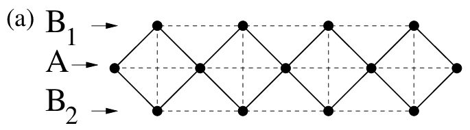
as sketched in Fig. 1(a). In Eq. (1), $\mathbf{A}_{l}$, $\mathbf{B}_{1l}$ and $\mathbf{B}_{2l}$ denote spin 1/2 operators at sites A_l, B_1l and B_2l of the unit cell $l$, respectively, and $N_{c}$ is the number of unit cells. For $J=0$ the model (named AB₂ chain or diagonal ladder) is bipartite and the Lieb-Mattis (LM) theorem [22] predicts a ground state (GS) total spin

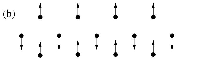
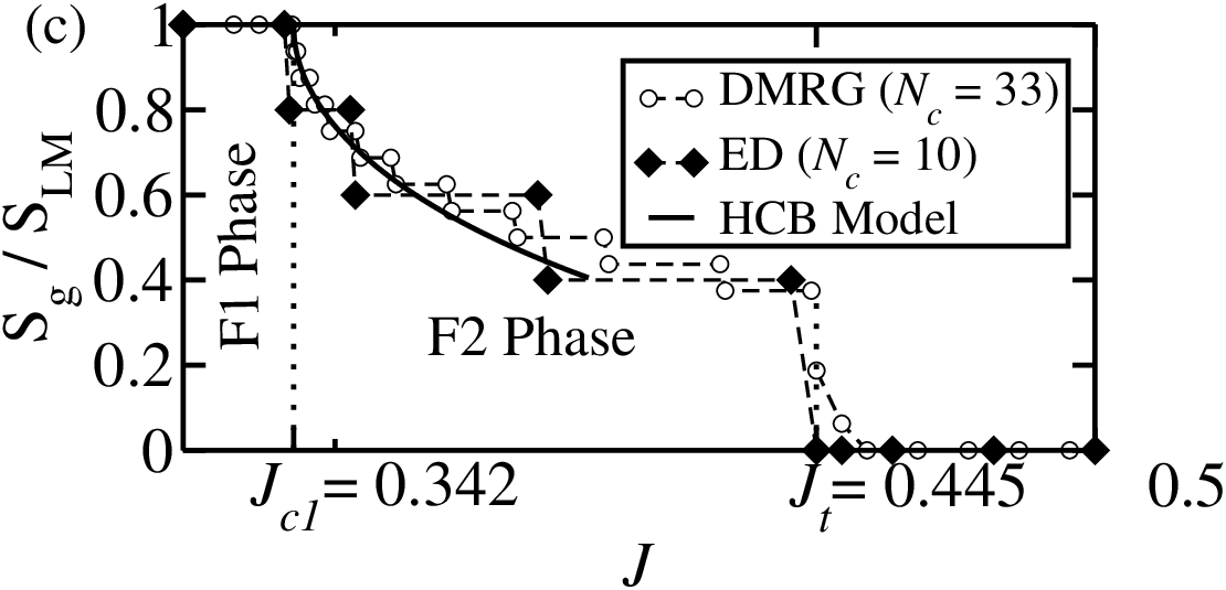
where $N_{A}$ ($N_{B}$) is the number of A (B₁ and B₂) sites. The GS spin pattern is represented in Fig. 1(b). In Fig. 1(c) we report data for $S_{g}/S_{LM}$ as a function of $J$ using DMRG ($N_{c}=33$) and ED ($N_{c}=10$). Although the LM theorem is not applicable for $J\neq 0$, the ferrimagnetic phase (F1 phase) is robust up to $J\approx 0.342\equiv J_{c1}$ (Ref. [23]), beyond which $S_{g}$ steadily decreases (F2 phase) before a first order transition to a phase with $S_{g}=0$ (apart from finite size effects) at $J\approx 0.445$.

In order to characterize the F2 phase, we have calculated the magnetic structure factor,

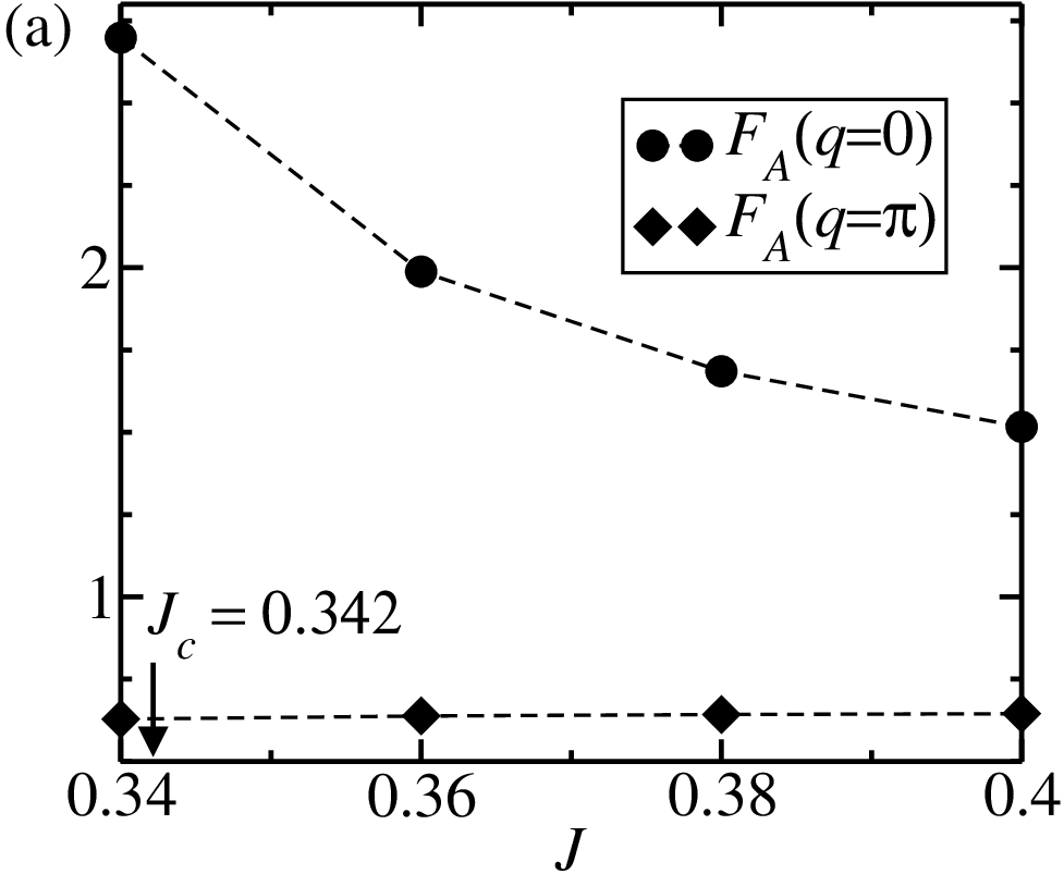
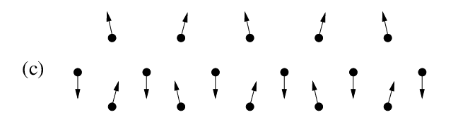
with $q=2\pi n/(N_{c}-1)$, $n=0,1,...,N_{c}-1$, where $C_{X}(l)$ is the two-point correlation function between spins separated by $l$ unit cells at sites $X=A,B_{1}\text{ and }B_{2}$. We first noticed that the A spins remain ferromagnetically ordered as the critical point $J_{c1}=0.342$ is crossed, although the magnitude of the peak at $q=0$ decreases for $J>J_{c1}$, as displayed in Fig. 2(a), while no peak is observed at $q=\pi$. The B_i ($i=1\text{ or }2$) spins also remain ferromagnetically ordered (peak at $q=0$), with similar $J$-dependence, as shown in Fig. 2(b). However, an extra peak at $q=\pi$ develops after the transition, which indicates the occurrence of a period-2 modulation in the spin pattern for $J\gtrsim J_{c1}$. Further, the average value of the correlation function $\langle\mathbf{B}_{1l}\cdot\mathbf{B}_{2l}\rangle$, which amounts to $\approx 0.25$ (triplet state) in the F1 phase, steadily decreases after the transition at $J_{c1}$. These findings suggest that the F2 phase would display a canted configuration, as illustrated in Fig. 2(c). However, to check whether these features are robust in the thermodynamic limit, we have studied the finite size scaling behavior of the transverse (T) and longitudinal (L) order parameters in the F2 phase:

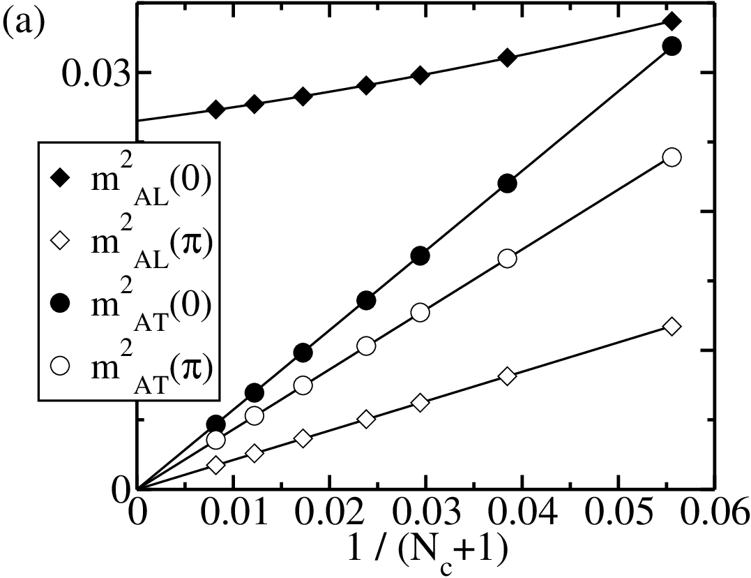
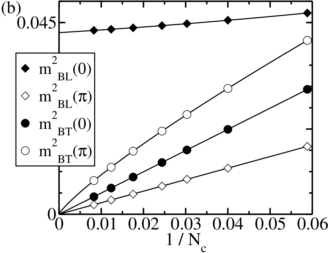
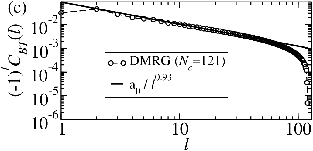
for $q=0$ (uniform component) and $q=\pi$ (staggered component), in the subspace of maximum total spin $z$-component ($S^{z}=S_{g}$). The correlations are studied at $J=0.395$, for which $S_{g}=S_{LM}/2$, and the results are shown in Fig. 3. We confirmed that in the (extrapolated) thermodynamic limit the spins at sites A and B are ferromagnetically ordered, as indicated by $m^{2}_{XL}(q=0)\neq 0$ in Figs. 3(a) and (b). Further, since the A and B net magnetizations are oppositely oriented, the F2 phase is ferrimagnetic. The values of $m^{2}_{AL}(q=\pi)$, $m^{2}_{BL}(q=\pi)$ and $m^{2}_{BT}(q=0)$ nullifies linearly with system size, which evidences short-range correlations. On the other hand, the best fitting to the data for $m^{2}_{BT}(q=\pi)$ presents a nonlinear dependence with the inverse of the system size and also nullifies in the thermodynamic limit. This behavior indicates that the staggered correlation function of the spins at sites B along the transverse direction to the spontaneous magnetization, $C_{BT\pi}(l)$, exhibits a power-law decay, as explicitly confirmed in Fig. 3(c). We thus conclude that for $J_{c1}<J<0.445$ the GS is also ferrimagnetic but with critical correlations along the transverse direction to the spontaneous magnetization (F2 phase).

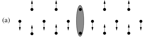
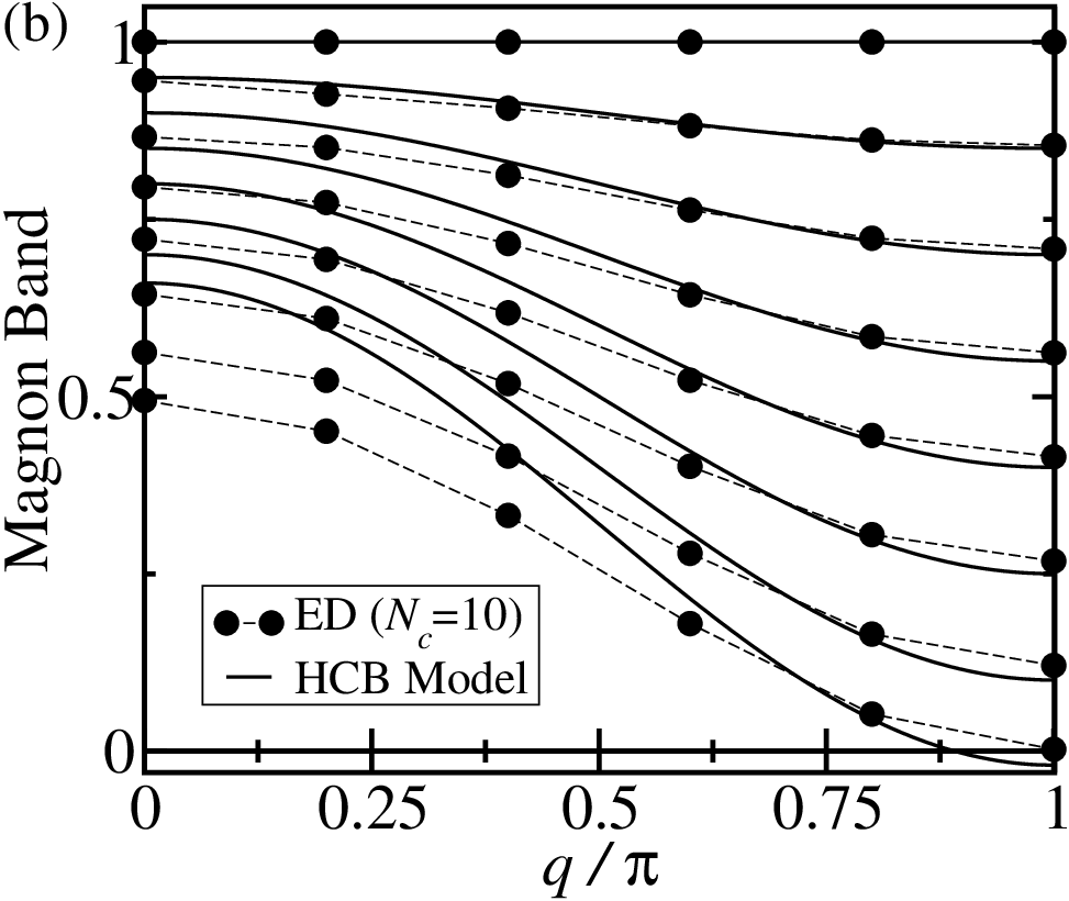
Next we focus on the effect of $J$ on the magnetic excitations. For $J=0$ the Hamiltonian exhibits three magnon modes [16, 15]. One is AF, i. e., the spin is raised by one unit with respect to the GS total spin, while the other two are ferromagnetic, associated with the lowering of the GS total spin by one unit. The AF gapped dispersive mode is responsible for a quantized plateau in the magnetization curve as function of $h$ and should also exhibit condensation, as suggested by the numerical data in Ref. [16]. One of the ferromagnetic magnons is the gapless dispersive Goldstone mode, while the other is a flat mode and is the relevant excitation for the transition at $J=J_{c1}$. To understand some nontrivial features of this excitation, we must comment on the symmetry properties of the model. For $J=0$ the Hamiltonian is invariant under the exchange of the B sites at the same cell. This symmetry implies that spins at these B sites can be found only in singlet or triplet states (mutually exclusive possibilities); in the GS only triplets are found. The relevant magnon is a localized gapped mode which induces the formation of a singlet pair in one cell, as illustrated in Fig. 4(a). For $J\neq 0$, this local symmetry is explicitly broken and the spins at these B sites can be found in a coherent superposition of singlet and triplet states. In Fig. 4(b), data using ED for the magnon band ($q=2\pi n/N_{c},n=0,1,...,N_{c}-1$) is displayed for various values of $J$ before the transition point. For $J=0$ the band is flat with a gap $\Delta_{0}\approx 1.0004$. By increasing $J$, the bandwidth increases and the gap to the GS lowers, closing at the wave vector $q=\pi$ at the transition point.

The GS total number of singlets is given by

with singlet density $\langle\eta_{l}\rangle=\langle s^{\dagger}_{l}s_{l}\rangle$, where

is the creation operator of a singlet pair at cell $l$ and $B_{il,\sigma}^{\dagger}$ is the creation operator of an electron with spin $\sigma$ at the B_i ($i=1,2$) site of cell $l$. In fact, it is easy to show that

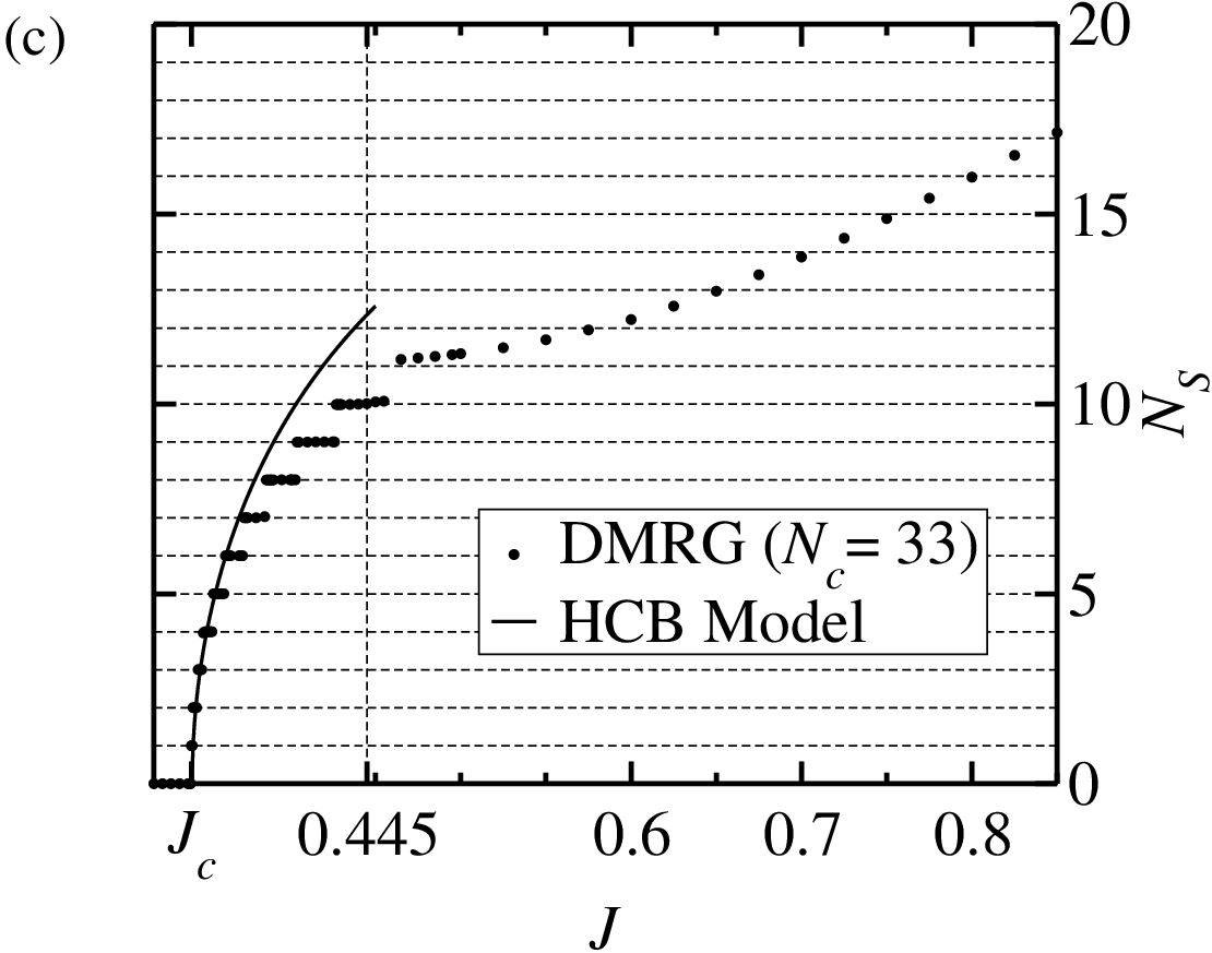
so $N_{S}=0$ for $J=0$. In Fig. 4(c) we observe that $N_{S}$ starts to increase in steps of unity after $J=J_{c1}$, indicating the quantized nature of the condensing singlets.

We now examine the nature of the quantum critical point at $J=J_{c1}$. For this purpose we split the Hamiltonian of Eq. (1) in three terms: the first favors ferrimagnetism,

where $\mathbf{S}_{l}=\mathbf{B}_{1l}+\mathbf{B}_{2l}$; the second one favors AF ordering between A spins, i. e.,

and shall play no significant role in our analysis; the last term, also unfavorable to ferrimagnetism, is a two-leg ladder Hamiltonian connecting spins at sites $B_{1}$ and $B_{2}$ (discarding a constant factor) [24, 25]:

where $\mathbf{D}_{l}=\mathbf{B}_{1l}-\mathbf{B}_{2l}$. We represent the Hamiltonian in a basis with two states for each pair $\mathbf{B}_{1l}$ and $\mathbf{B}_{2l}$: the singlet and the triplet component in the magnetization direction. In addition, we define the vacuum of the HCB model as the state with this triplet component in each cell. We now study the GS energy when a number $N_{S}$ of singlet pairs is added to the vacuum. For $J=0$, the energy cost of a singlet pair is $\Delta_{0}$ (the gap to the flat mode); thus, for $N_{S}$ singlets, the contribution from $H_{AB}$ is $N_{S}\Delta_{0}$. The first term in $H_{B}$ is diagonal and will add a factor of $-JN_{S}$; the second causes a repulsion between singlets and adds also an extra factor of $-JN_{S}$; finally, the last term in $H_{B}$ introduces the singlet itinerancy. Grouping these contributions, we arise to a model of hard-core bosons with nearest-neighbor repulsion:

We remark that the hard-core boson interaction is implied by the algebra of the singlet operators:

Before the transition, the single magnon dispersion relation,

agrees well with the numerical data for $q\approx\pi$, as can be seen in Fig. 4(b). The resulting critical point: $\omega_{q=\pi}(J_{c1,S})=0$, i. e.,

is in excellent agreement with the numerical prediction $J_{c1}=0.342$. Moreover, the closing of the magnon gap is also in excellent agreement with the prediction

and with the expected linear vanishing of the Mott gap [26]: $z\nu=1$, where $z=2$ and $\nu=1/2$ are the correlation length and dynamic critical exponents, respectively (see below).

After the transition and in the highly diluted limit ($\frac{N_{S}}{N_{c}}\equiv\eta\rightarrow 0$), the energy of $N_{S}$ hard-core bosons in 1D is well approximated by the energy of $N_{S}$ free spinless fermions [5]. Through this map, the energy density reads:

where $k_{F}=\pi\eta$ and

Notice that the Fermi chemical potential satisfies the Tonks-Girardeau (TG) limit [27, 7, 28] (1D Bose gas of impenetrable particles), corresponding to an infinitely high repulsive potential in the Lieb-Liniger solution [29] of the $\delta$-function 1D Bose gas:

where $J^{-1}$ is the fermion mass, $\hbar\equiv 1$, and $\eta$ is the density of singlets for $J\geq J_{c1,S}$ derived from the equilibrium condition $\partial_{\eta}\mathcal{E}_{GS}(J)=0$:

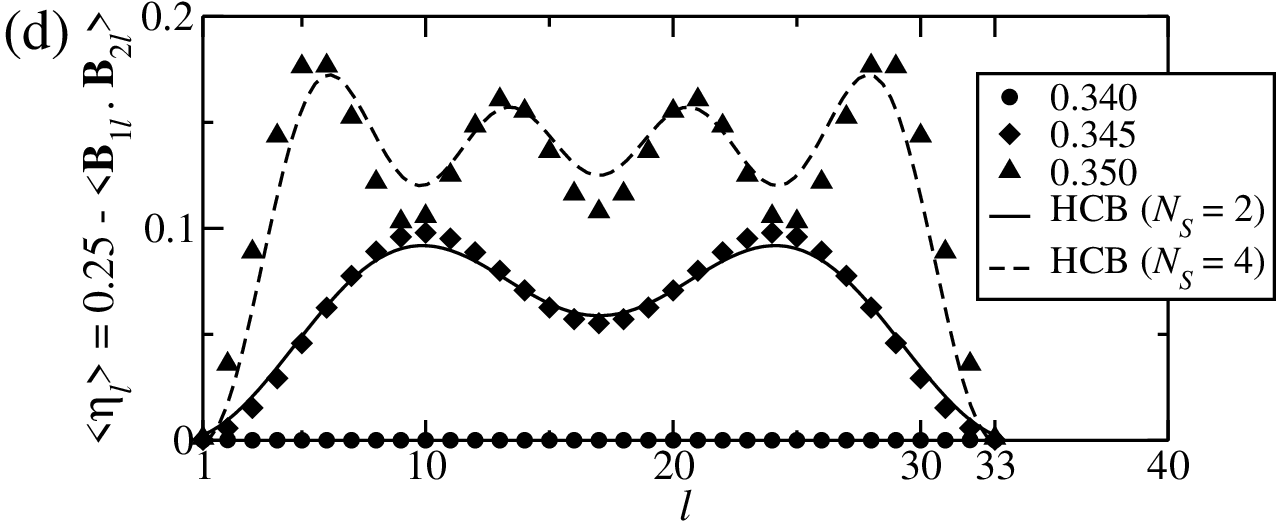
much in analogy with the 1D field-induced transition. Further, in Fig. 4(d) we display the good agreement between the numerical estimate for the density $\langle\eta_{l}\rangle$ of a two (four) particle state, $N_{S}=2$ ($N_{S}=4$), in an open system and the HCB model in a continuum space given by [24]

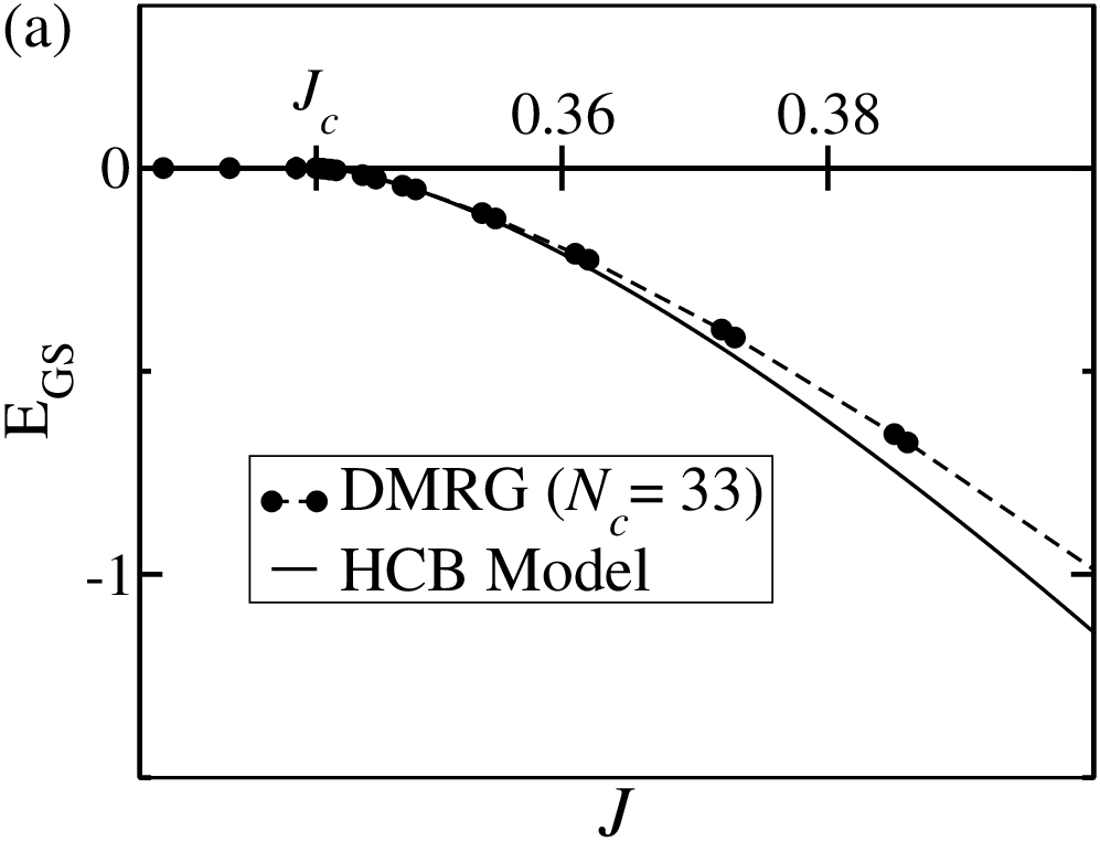
with $k_{n}=1,...,\frac{\pi N_{S}}{N_{c}-1}$. Also, as shown in Figs. 1(c), 4(c) and 5(a), the HCB model predictions for

$\eta$ and $E_{GS}(J)$, respectively, are very close to the numerical data for $J\gtrsim J_{c1}\approx J_{c1,S}$.

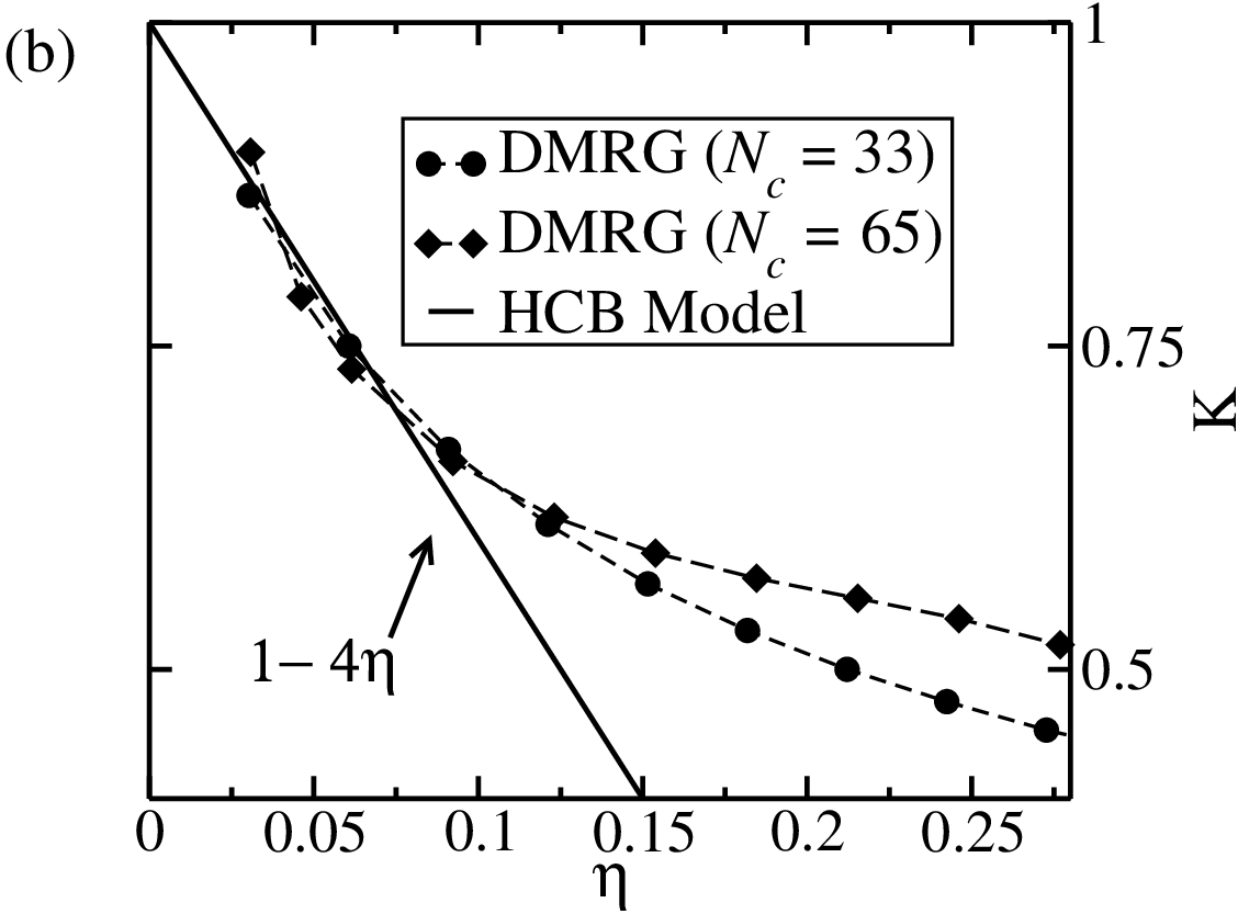
On the other hand, using the Luttinger liquid description [30, 31] for our highly diluted HCB model we have the following general relations for the sound velocity $c$ and the compressibility $\kappa$:

where $K$ is the Luttinger parameter governing the decay of the correlation functions. However, since

it implies that $K=1$; thus $c=\pi J\eta=Jk_{F}$, in accord with the TG limit [7, 28]. Further, taking $\eta$ as the order parameter of the SIT, Eq. (21) implies $\beta=1/2$, while $\eta^{2}\kappa$ diverges with a critical exponent $\alpha=\gamma=1/2$, in agreement with the scaling and hyperscaling relations [26]:

respectively, assuring that the SIT is in the free spinless gas universality class [32].

In an interacting Bose gas [33], $K=1/2$ is the separatrix between systems dominated by superfluid fluctuations, $K>1/2$, from those dominated by charge density fluctuations, $K<1/2$, (in our magnetic model spin fluctuations prevail). Affleck and collaborators [34] have succeeded in taking into account corrections from interactions between pairs of dilute magnons parametrized by a scattering length, $a$, thus implying that

where $m$ is the field-induced magnetization for the $S=1$ chain, with $a\approx-2$. The predicted increase of $K$ with $m$ was confirmed by numerical calculations [34]. This parametrization can also be implemented in our problem. In fact, in Fig. 5(b) we show that $K=1-4\eta$, with $a\approx 2$, fits quite well the data for the Luttinger liquid parameter in the highly diluted regime. $K$ was calculated using DMRG and assuming

We now turn our attention to the transition point $J_{t}\approx 0.445$, which marks the onset of a singlet phase, as can be seen in Fig. 1(c), characterized by non-quantized values of $N_{S}$, as shown in Fig. 4(c). On the other hand, from the Hamiltonians in Eqs. (8)-(10), we can infer that for $J>>1$ the system should decompose into a linear chain (A sites) and an isotropic two-leg ladder system (B₁ and B₂ sites); see Fig. 1(b). The linear chain is known to be gapless with critical spin correlations (power-law decay), while the two-leg ladder is gapped with exponentially decaying correlations. In what follows we discuss the complex phase diagram in the region $J>J_{t}$.

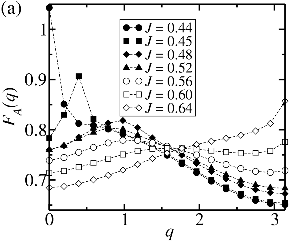
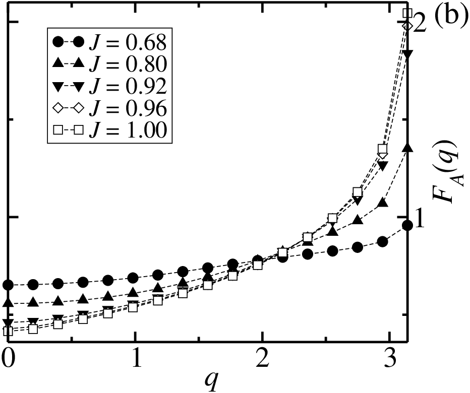
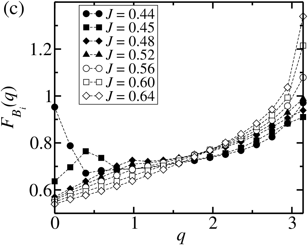
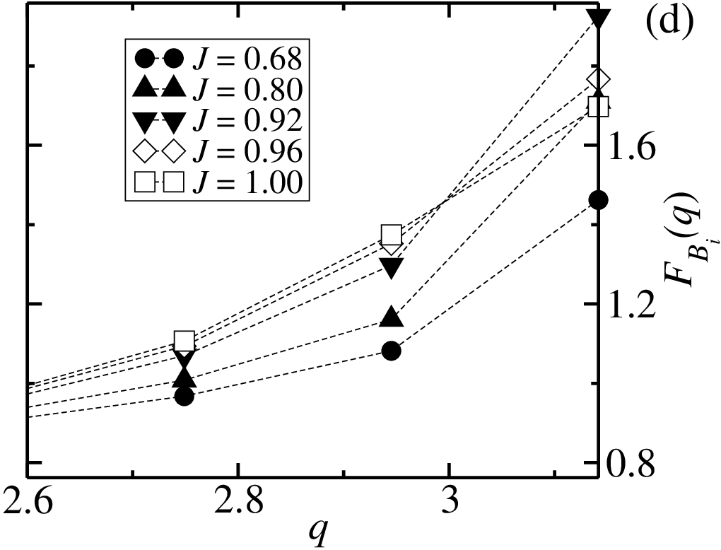
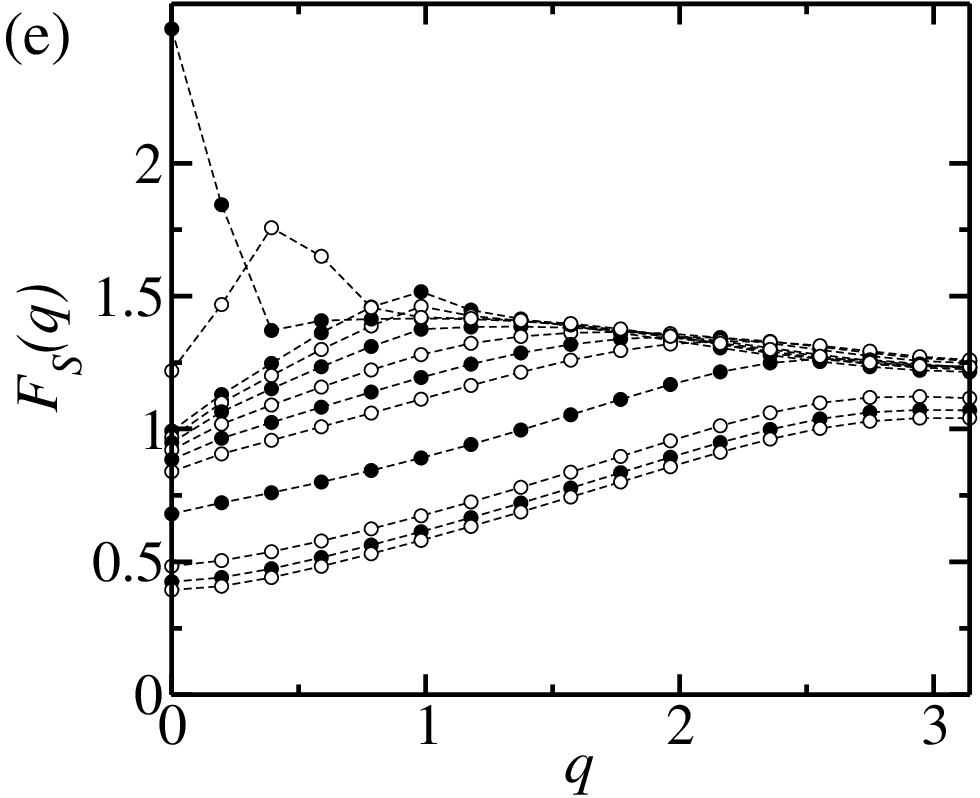
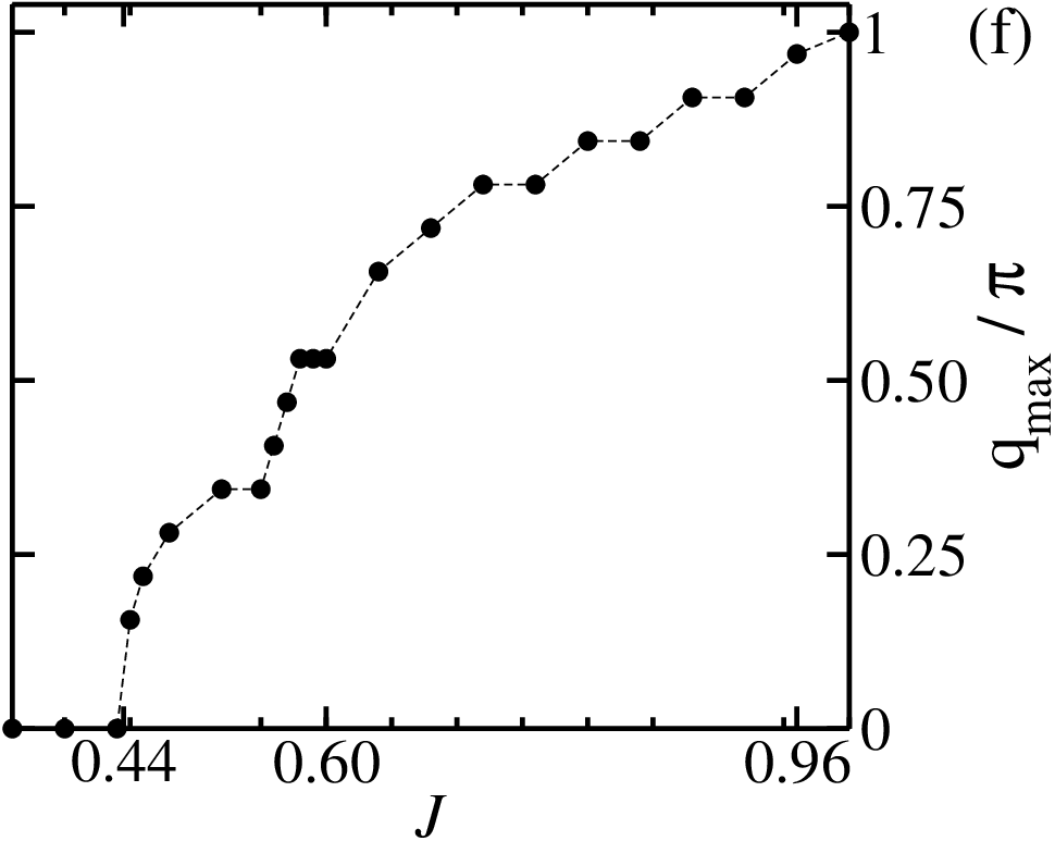
Initially, we display in Fig. 6 the magnetic structure factors $F_{A}(q)$ and $F_{B_{i}}(q)$, with $i=1\text{ or }2$, as well as $F_{S}(q)$, which is associated to the magnetic structure of the composite spin $\mathbf{S}_{l}=\mathbf{B}_{1l}+\mathbf{B}_{2l}$. In Fig. 6(a) we see that $F_{A}(q)$ peaks at $q=0$ for $J=0.44$, i. e., the system remains in the F2 phase and the A spins are ferromagnetically ordered. For $J=0.45$, a sharp peak in a spiral wave-vector $q_{max}$ is observed. The peak broadens and $q_{max}$ increases with increasing $J$. For $J=0.56$ we notice the emergence of a commensurate AF peak, coexisting with the spiral one, particularly for $J\geq 0.60$, as seen in Figs. 6(a) and 6(b). On the other hand, we observe in Fig. 6(c) the presence of two peaks in $F_{B_{i}}(q)$ for $J=0.44$: the $q=0$ peak associated with the ferromagnetic ordering of the $B_{i}$ sites in the F2 phase, and the $q=\pi$ peak related to the critical staggered transverse correlation at the same phase. Likewise, for $J=0.45$, a spiral peak is observed at the same wave-vector $q_{max}$ of $F_{A}(q)$. Further, notice in Fig. 6(d) that the magnitude of the AF peak drops in the interval $0.96\leq J<1.00$.

In order to develop a physical meaning of the above referred data, we first point out that the coupling between spins at A and B sites occurs through the composition $\mathbf{S}_{l}=\mathbf{B}_{1l}+\mathbf{B}_{2l}$, as can be seen in Eq. (8). Further, as the singlet component of $\mathbf{S}_{l}$ is magnetically inert, only its triplet components affect the magnetic ordering at the A sites. In fact, as shown in Figs. 6(e) and 6(f), short-range spiral ordering is observed in the magnetic structure of $\mathbf{S}_{l}$ up to $J\approx 1.00$. However, since the peak is weak and broad for $J\gtrsim 0.6$, its feature is overcomed by the AF one in the data of Figs. 6 [(a)-(d)]. In the sequence, we focus on the AF ordering observed for $J\gtrsim 0.6$ and study how the system approaches the ladder-chain decoupling.

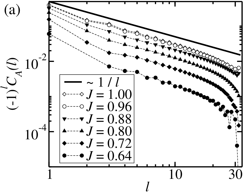
In Fig. 7(a), we present the staggered AF correlation function between A-spins as $J\rightarrow 1$. As observed, its behavior is well described by that found in a single linear chain, which is asymptotically given by

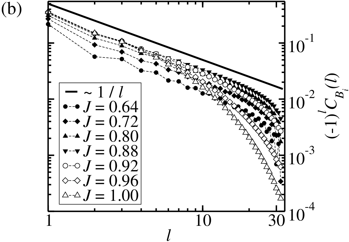
apart from logarithmic corrections [30]. A similar behavior is observed in Fig. 7(b) for the staggered AF correlation between $B_{i}$-spins up to $J=0.88$, a value beyond which the shape of the curve is visibly changed. In order to understand this dramatic behavior, we recall that in a two-leg ladder system the asymptotic form of the correlation is given by [35]

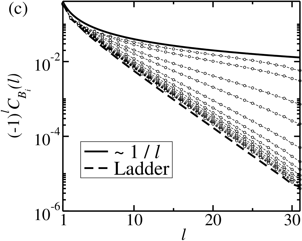
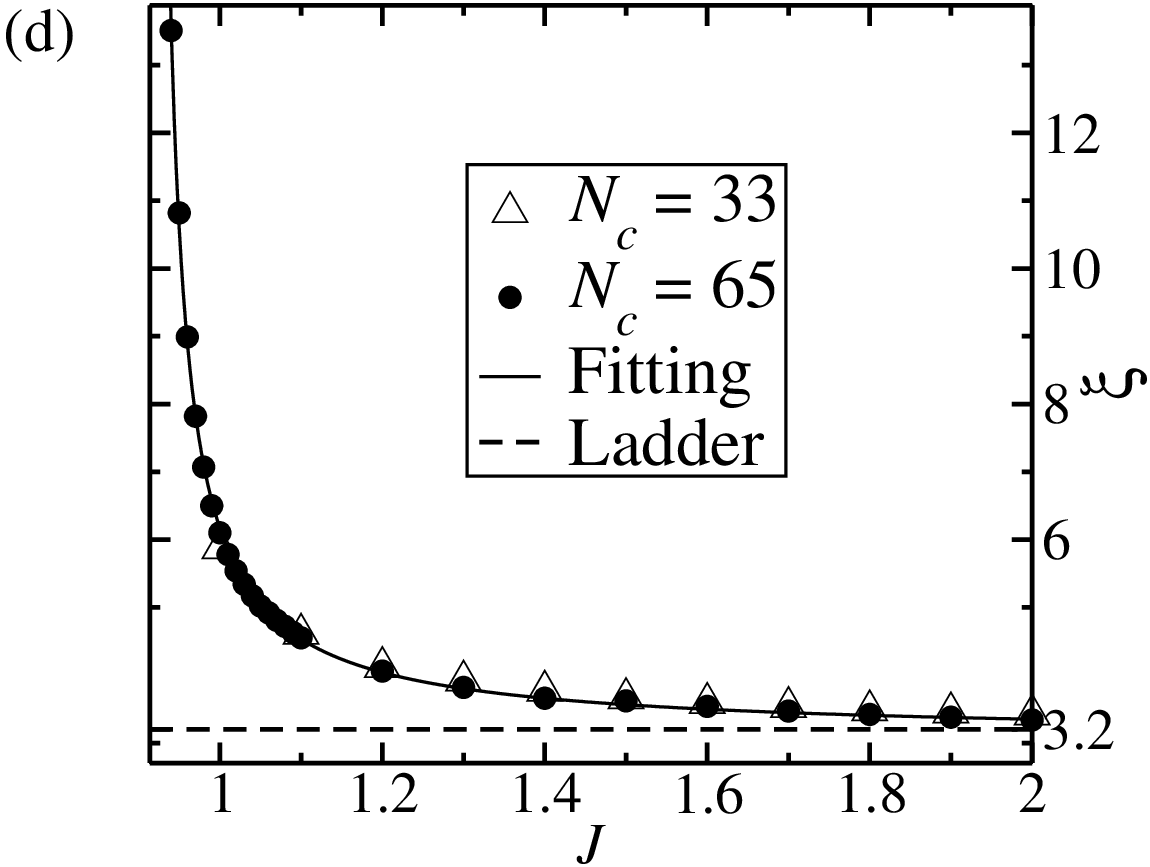
where $\xi(\approx 3.2,\text{see Ref.\cite[cite]{[\@@bibref{Number}{WhitePRL1994}{}{}]}})$ defines the correlation length, associated with the gapped spin liquid state of this system. Indeed, as displayed in Fig. 7(c) the staggered correlations $C_{B_{i}}$ asymptotically approaches the correlation in a two-leg ladder system. In Fig. 7(d) we present the behavior of $\xi$ as a function of $J$ for $N_{c}=33$ and $N_{c}=65$. These data were obtained by a proper fitting of $C_{B_{i}}$ in the interval $l_{0}<l<(N_{c}/2)$: starting from $J=2$ and taking $l_{0}\approx 6$ (about twice the value of $\xi$ of a two-leg ladder), we find $\xi$; twice this value of $\xi$ was used as input ($l_{0}=2\xi$) for the next chosen value of $J$, and so on. Moreover, we have obtained a good fitting to these data by using the two-loop analytic form of the O(3) non-linear sigma model (NLSM) correlation length in (1+1) dimension [37]:

where $a$ is a constant and $g$ is the NLSM coupling. Further, we assume (see below) that the coupling $g$ is the one suitable to the anisotropic quantum Heisenberg two-leg ladder to the NLSM [38]:

where $J_{\perp}$ ($J_{\parallel}$) is the exchange coupling between spins at the same rung (leg) and $\kappa$ is a constant that depends on the choice of the lattice regularization.

In order to justify Eq. (34) for $g$, we consider a mapping of the model Hamiltonian, Eq. (1), to the Hamiltonian of an isolated two-leg ladder by eliminating the spin degrees of freedom associated with the A sites. The mapping is performed, in a semiclassical manner, by the following assumption on $H_{AB}$ [Eq. (8)]:

where $\gamma$ is an effective coupling constant. This amounts to reduce the A-B coupling to spins within the same unit cell, and cell-cell interactions are taken into account through the effective coupling $\gamma$. We now write: $(\mathbf{A}_{l}+\mathbf{S}_{l})^{2}=\mathbf{A}_{l}^{2}+\mathbf{S}_{l}^{2}+2\mathbf{A}_{l}\cdot\mathbf{S}_{l}$, with $\mathbf{S}_{l}^{2}=\mathbf{B}_{1l}^{2}+\mathbf{B}_{2l}^{2}+2\mathbf{B}_{1l}\cdot\mathbf{B}_{2l}$; since within a unit cell $(\mathbf{A}_{l}+\mathbf{S}_{l})^{2}\approx(1/2)^{2}$ in an AF phase, and dropping constant terms, $\overline{H}_{AB}$ can be written as

Since correlations between spins at $A$ sites does not play a significant role close to the transition, we discard the term $H_{A}$, and, finally, obtain the following anisotropic two-leg ladder Hamiltonian:

where the exchange couplings are given by

Substituting Eqs. (38) and (39) into Eq. (34), we find the effective NLSM coupling:

where $J_{c2}=\gamma/3$. We have fitted the data in Fig. 7(d) to Eq. (33), with $g$ given by Eq. (40), and $a$, $\kappa$ and $J_{c2}$ as fitting parameters. The obtained value of $a$ (=2.7) is such that $\xi\rightarrow 3.1$ as $J\rightarrow\infty$, which agrees with the expected value for an isolated isotropic two-leg ladder ($\approx 3.2$), while $\kappa=4.5$ and $J_{c2}=0.91$, in agreement with the correlation function behavior shown in Fig. 7(b).

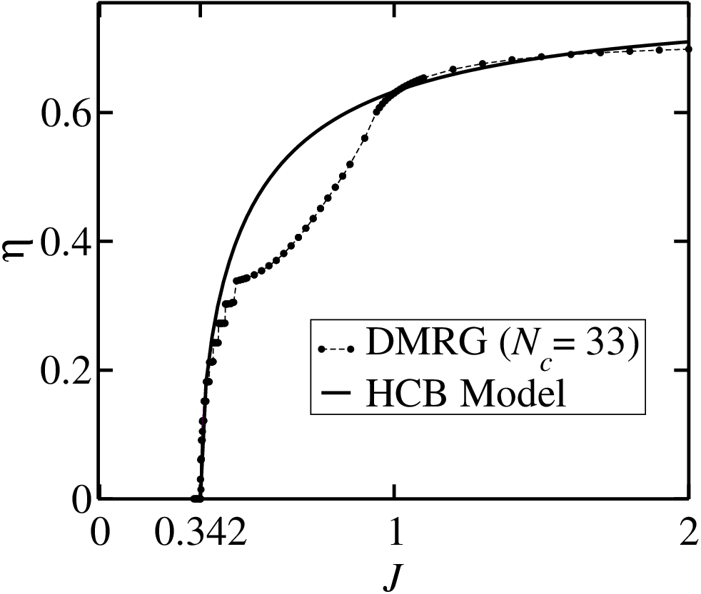
Finally, in Fig. 8 we display the very interesting behavior of the density of singlets, $\eta$, as function of $J$. It is clear that the effect of the A-spins and singlet-singlet interaction is relevant only for $J_{t}\lesssim J\lesssim J_{c2}$, otherwise the solution, Eq. (21), for low density of singlets can be extended to the region of low density of triplets above $J_{c2}$ (strongly coupling limit), where correlations between B-spins are exponentially small [see Eq. (32)]. In fact, the asymptotic value predicted by Eq. (21), i. e., $\eta=\sqrt{6}/\pi\approx 0.78$, compares well with the numerical one: $\approx 0.71$.

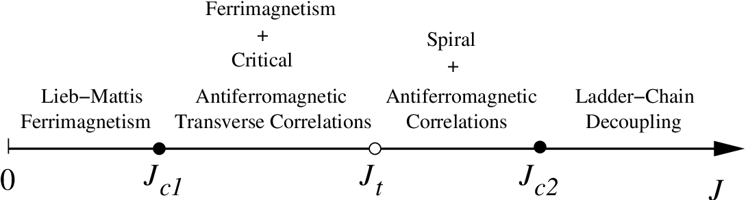
In this work we have derived the rich phase diagram of a three-leg spin Hamiltonian related to quasi-one-dimensional ferrimagnets, as function of a frustration parameter $J$ which destabilizes the ferrimagnetic phase. In Fig. 9 we present an illustration of the obtained phase diagram, which displays two critical points, $J_{c1}\approx 0.342$ and $J_{c2}\approx 0.91$, and a first order transition point at $J_{t}\approx 0.445$. Through DMRG, exact diagonalization and a hard-core boson model, we have characterized the transition at $J_{c1}$ as an insulator-superfluid transition of magnons (built from the coherent superposition of singlet and triplet states between B sites at lattice unit cells), with a well defined Tonks-Girardeau limit in the high diluted regime. Ferrimagnetism with critical staggered correlations in a direction transverse to the spontaneous magnetization is observed for $J_{c1}<J<J_{c2}$. Further, for $J_{c1}<J<J_{t}$ the number of singlets in the lattice is quantized, while above the first order transition at $J=J_{t}$ this quantity is a continuous one. Also, in the interval $J_{t}<J<J_{c2}$ the magnetic structure factor displays a singlet phase with incommensurate ($q\neq 0\text{ and }\pi$) spiral and AF peaks. However, the spiral peak broads and the AF peak is the salient feature as $J$ increases within this phase. At $J=J_{c2}$ a remarkable gapped two-leg ladder / critical single-linear chain decoupling transition occurs, characterized by an essential singularity in the correlation length as predicted by the NLSM through a mapping of our model onto an anisotropic quantum Heisenberg two-leg ladder. For $J\gg J_{c2}$ the ladder approaches the isotropic limit (full decoupling), while the linear chain remains critical.

In summary, our reported results clearly reveal that frustrated quasi-one-dimensional magnets are quite remarkable systems to study magnon condensation, including the crossover to coupled ladder systems of higher dimensionality [39] and related challenging phenomena [40], as well as frustration-driven quantum decoupling transition in ladder systems.

We acknowledge useful discussions with A. S. F. Tenório and E. P. Raposo. This work was supported by CNPq, Finep, FACEPE and CAPES (Brazilian agencies).

References

- [1] M. Jaime et al., Phys. Rev. Lett 93, 087203 (2004); T. Radu, H. Wilhelm, V. Yushankhai, D. Kovrizhin, R. Coldea, Z. Tylczynski, T. Lühmann, and F. Steglich, Phys. Rev. Lett. 95, 127202 (2005); V. S. Zapf et al., Phys. Rev. Lett. 96, 077204 (2006); V. O. Garlea et al., Phys. Rev. Lett. 98, 167202 (2007).
- [2] Ch. Ruegg et al., Phys. Rev. Lett. 93, 257201 (2004).
- [3] S. O. Demokritov et al., Nature 443, 430 (2006).
- [4] J. Kasprzak et al., Nature 443, 409 (2006); R. Balili et al., Science 316, 1007 (2007).
- [5] I. Affleck, Phys. Rev. B 43, 3215 (1991); E. S. Sorensen and I. Affleck, Phys. Rev. Lett. 71, 1633 (1993); see also A. M. Tsvelik, Phys. Rev. B 42, 10499 (1990).
- [6] T. Giamarchi and A. M. Tsvelik, Phys. Rev. B 59, 11398 (1999).
- [7] L. Pitaevskii and S. Stringari, Bose-Einstein Condensation (Clarendon Press, New York, 2003).
- [8] D. Snoke, Nature 443, 403 (2006).
- [9] M. D. Coutinho-Filho, R. R. Montenegro-Filho, E. P. Raposo, C. Vitoriano, and M. H. Oliveira, J. Braz. Chem. Soc. 19, 232 (2008).
- [10] M. Matsuda et al., Phys. Rev. B 71, 144411 (2005).
- [11] Y. Hosokoshi et al., J. Am. Chem. Soc. 123, 7921 (2001).
- [12] A. M. S. Macêdo, M. C. dos Santos, M. D. Coutinho-Filho, and C. A. Macêdo, Phys. Rev. Lett. 74, 1851 (1995); G.-S. Tian and T.-H. Lin, Phys. Rev. B 53, 8196 (1996).
- [13] G. Sierra, M. A. Martín-Delgado, S. R. White, D. J. Scalapino, and J. Dukelsky, Phys. Rev. B 59, 7973 (1999).
- [14] F. C. Alcaraz and A. L. Malvezzi, J. Phys. A: Math. Gen. 30, 767 (1997); E. P. Raposo and M. D. Coutinho-Filho, Phys. Rev. Lett. 78, 4853 (1997); Phys. Rev. B 59, 14384 (1999); M. A. Martín-Delgado, J. Rodriguez-Laguna, and G. Sierra, Phys. Rev. B 72, 104435 (2005).
- [15] C. Vitoriano, F. B. de Brito, E. P. Raposo, and M. D. Coutinho-Filho, Mol. Cryst. Liq. Cryst. 374, 185 (2002); T. Nakanishi and S. Yamamoto, Phys. Rev. B 65, 214418 (2002); S. Yamamoto and J. Ohara, Phys. Rev. B 76, 014409 (2007).
- [16] R. R. Montenegro-Filho and M. D. Coutinho-Filho, Physica A 357, 173 (2005).
- [17] R. R. Montenegro-Filho and M. D. Coutinho-Filho, Phys. Rev. B 74, 125117 (2006), and references therein.
- [18] H. Kikuchi, Y. Fujii, M. Chiba, S. Mitsudo, T. Idehara, T. Tonegawa, K. Okamoto, T. Sakai, T. Kuwai and H. Ohta, Phys. Rev. Lett. 94, 227201 (2005). See also: K. C. Rule, A. U. B. Wolter, S. Süllow, D. A. Tennant, A. Brühl, S. Köhler, B. Wolf, M. Lang, and J. Schreuer, Phys. Rev. Lett. 100, 117202 (2008).
- [19] K. Okamoto, T. Tonegawa, and M. Kaburagi, J. Phys. Condens. Matter 15, 5979 (2003).
- [20] S. R. White, Phys. Rev. B 48, 10345 (1993); U. Schollwöck, Rev. Mod. Phys. 77, 259 (2005).
- [21] In the DMRG calculation we have retained from 300 to 1080 states per block. The discarded density matrix weight ranges from 10-10 to 10-7, typically 10-8.
- [22] E. Lieb and D. Mattis, J. Math. Phys. 3, 749 (1962).
- [23] A similar behavior was observed in a frustrated ferrimagnetic ladder: N. B. Ivanov and J. Richter, Phys. Rev. B 69, 214420 (2004).
- [24] J.-B. Fouet et al., Phys. Rev. B 73, 214405 (2006).
- [25] T. Hikihara and A. Furusaki, Phys. Rev. B 63, 134438 (2001).
- [26] M. P. A. Fisher, P. B. Weichman, G. Grinstein, and D. S. Fisher, Phys. Rev. B 40, 546 (1989).
- [27] L. Tonks, Phys. Rev. 50, 955 (1936); M. Girardeau, J. Math. Phys. 1, 516 (1960).
- [28] The TG limit has been observed in ultracold 87Rb atoms: Paredes et al., Nature 429, 277 (2004); T. Kinoshita, T. Wenger, D. S. Weiss, Science 305, 1125 (2004); Phys. Rev. Lett. 95, 190406 (2005).
- [29] E. H. Lieb and W. Liniger, Phys. Rev. 130, 1605 (1963).
- [30] J. Voit, Rep. Prog. Phys. 58, 977 (1995).
- [31] I. Affleck, W. Hofstetter, D. R. Nelson and U. Schollwöck, J. Stat. Mech.: Theor. Exp., P10003 (2004).
- [32] S. Sachdev, T. Senthil, and R. Shankar, Phys. Rev. B 50, 258 (1994).
- [33] T. Giamarchi, AIP Conf. Proc. 846, 94 (2006).
- [34] J. Lou, S. Qin, T.-K. Ng, Z.-B. Su, and I. Affleck, Phys. Rev. B 62, 3786 (2000); I. Affleck, Phys. Rev. B 72, 132414 (2005).
- [35] D. G. Shelton, A. A. Nersesyan, A. M. Tsvelik, Phys. Rev. B 53, 8521 (1996).
- [36] S. R. White, R. M. Noack, and D. J. Scalapino, Phys. Rev. Lett. 73, 886 (1994).
- [37] E. Brézin and J. Zinn-Justin, Phys. Rev. B 14, 3110 (1976); S. H. Shenker and J. Tobochnik, Phys. Rev. B 22, 4462 (1980).
- [38] D. Sénéchal, Phys. Rev. B 52, 15319 (1995); G. Sierra, J. Phys. A 29, 3299 (1996); G. Sierra, in Strongly Correlated Magnetic and Superconducting Systems, Lecture Notes in Physics Vol. 478, edited by G. Sierra and M. A. Martín-Delgado (Springer-Verlag, Berlin, 1997) (cond-mat/9610057); S. Dell’Aringa, E. Ercolessi, G. Morandi, P. Pieri, and M. Roncaglia, Phys. Rev. Lett. 78, 2457 (1997).
- [39] E. Orignac, R. Citro, and T. Giamarchi, Phys. Rev. B 75, 140403(R) (2007).
- [40] S. E. Sebastian et al., Nature 441, 617 (2006); P. A. Sharma, N. Kawashima, and I. R. Fisher, Nature (London) 441, 617 (2006).