How precisely neutrino emission from supernova remnants
can be constrained by gamma ray observations?

Under-water and under-ice neutrino telescopes are instruments aiming to discoveries. They could reveal an effective acceleration of cosmic rays (CR) in galactic sources (such a supernova remnants [1] and micro-quasars [2]) and/or in extragalactic sources (such as AGN and gamma ray bursts [3]). However, at present it is possible to obtain reliable expectations only for few of these sources, such as the supernova remnants (SNR) discussed in this paper.

The idea that CR could originate in supernovae has been put forward already in 1934 but the first quantitative formulation of the conjecture that the young SNRs refurnish the Milky Way of cosmic rays, compensating the energy losses, is due to Ginzburg & Syrovatskii [1]. In fact, the turbulent gas of SNRs is a large reservoir of kinetic energy and this environment can support diffusive shock waves acceleration  [4]. The theory of CR acceleration in SNRs is still in evolution, but the generic expectations are stable. The CR flux in SNRs is expected to have a power law spectrum with spectral index $\Gamma=2.0-2.4$ at low energies with a cutoff at an energy $E_{\rm c}$ which depends on the details of the acceleration mechanism and on the age of the system. In specific implementations the cutoff energy $E_{\rm c}$ can be as large as several PeV and, thus, is consistent with the “knee” in the CR spectrum at $E\sim 3\times 10^{15}\,{\rm eV}$, which is believed to mark the transition from galactic to extra-galactic origin of CR  [5].

In recent times, great progress has been made in the observation of SNRs. In particular, the High Energy Stereoscopic System (H.E.S.S.) [6] has determined quite precisely the gamma ray spectra of few SNRs showing that they extend above 10 TeV. In the context of Ginzburg & Syrovatskii hypothesis, it is natural to postulate that the observed gammas are produced by the decay of $\pi^{0}$ (and $\eta$) resulting from the collision of accelerated hadrons with the ambient medium. New and crucial observations are being collected and the hadronic origin seems to be favored for certain SNRs, such as Vela Jr [7] and RX J1713.7-3946 [8, 9].¹¹ 1 See also [10] for a recent analysis leading to a different conclusion. It is not yet possible, however, to exclude that (part of) the observed radiation is produced by electromagnetic processes. The definitive proof that SNRs effectively accelerate CR could be obtained by the observation of high energy neutrinos in neutrino telescopes presently in operation, in construction or in project [11].

As well known, there is a strict connection between photon and neutrino fluxes produced by hadronic processes in transparent sources (see, e.g.,  [12]), which results from the fact that the same amount of energy is roughly given to $\pi^{0}$, $\pi^{+}$ and $\pi^{-}$ in hadronic collisions. On this basis, one can estimate the neutrino fluxes expected from a sources with known $\gamma$-ray spectra, trying to identify detectable sources and/or to optimize the detection strategies. The gamma-neutrino connection has been described in various recent papers [13, 14, 15, 16, 18, 19, 20, 21] at a different level of accuracy, relying on different assumptions on the primary cosmic ray spectrum and/or hadronic interaction model.

In this particular moment, when high energy gamma ray astronomy is flourishing and the neutrino telescopes are finally becoming a reality, it is clearly important to have solid and transparent predictions. We continue, thus, the work started in [16, 21, 22], proposing a method to calculate neutrinos fluxes which is, at the same time, simple, accurate and model-independent. Our results are in essence a straightforward applications of standard techniques [23], but we believe that that they will be useful since they improve the existing calculations in various respects. In particular, we provide simple analytic expressions for the neutrino fluxes which have a general validity and can be applied directly to gamma ray data since they do not require any parametrization of the photon spectrum. This allows us to propagate easily the observational errors in the gamma ray flux and, thus, to understand how well the neutrino flux and the signal in neutrino telescopes can be constrained by $\gamma$-ray data. We also discuss the various possible sources of theoretical and systematical uncertainties, obtaining an estimate of the accuracy of our method. This kind of analysis is relevant in the present situation, since the number of events expected in neutrino telescopes from SNRs is quite low (see, e.g., [16]) and even small (downward) revisions of the expected signals may be important and/or require different detection strategies. It is thus important to understand the relevance of different assumptions in the calculations and the origin of (apparently) contrasting results appeared in the literature.

The plan of the paper is as follow. In Sect. 2 we review the method presented in our previous paper  [16]. The relations obtained in this work – Eqs. (8) – are physically equivalent to those presented in [16]. However, they are more compact and more convenient for numerical computations since we have been able to recast them in such a way that they require only one numerical integration. In Sect. 3, we discuss the effect of neutrinos oscillations (see [24] for a review) and we discuss the relevance of uncertainty in neutrino mixing parameters for the predicted neutrino flux. In Sect. 4 we present our main results, i.e., Eqs. (30) and (32) which relate the (oscillated) muon neutrino and antineutrino fluxes to the $\gamma$-ray flux. As it is explained, the only necessary information to predict neutrino fluxes are the relative production rates of the various mesons in hadronic processes, which are robust predictions of hadronic interaction models. In this paper, we adopt the results from Pythia [25], estimated by using the parametrization of hadronic cross sections presented in [26]. A comparison with SYBILL  [27] and DPMJET-III [28] is performed (when possible) by using the parametrization and tabulations of hadronic cross sections presented by [29] and [30]. In Sect. 5 and 6 we propose a procedure to predict neutrino fluxes and event rate in $\nu$-telescopes directly from $\gamma$-ray observational data, and we apply it to RX J1713.7-3946 which is presently the best studied SNR. In Sect. 7 we summarize our main results.

The interactions of cosmic ray protons with a hydrogen ambient cloud result in the production of mesons which subsequently decay producing gamma ray and neutrinos. Both gamma rays and neutrinos depend linearly on the flux of the primary cosmic ray. We, thus, expect that a linear relation also exists between photon and neutrino fluxes, which can formally be expressed as:

$$\Phi_{\nu}[E_{\nu}]=\int\frac{dE_{\gamma}}{E_{\gamma}}\;K_{\nu}[E_{\nu},E_{\gamma}]\,\Phi_{\gamma}[E_{\gamma}].$$

as will be precised just below in this Section.

In order to determine the kernels $K_{\nu}[E_{\nu},E_{\gamma}]$, we only need to know the relative number of pions, kaons and $\eta$ produced by cosmic rays at any given energy, as it is explained in [16] and further discussed in the following. Let us indicate with $R_{i}[E]$ the number of $i-$particles produced per unit time and unit energy in the cloud. Here, for simplicity, we assume that the momentum distributions of the various particles are approximately isotropic, so that the differential flux produced in a detector at a distance $D$ (if the $i-$particle is stable) is simply given by:²² 2 If this assumption is removed, one has to replace here and in the following: $$\frac{1}{4\pi}R_{i}[E]\longrightarrow\frac{dR_{i}[E,{\bf n}]}{d\Omega}$$ where $dR_{i}/{d\Omega}$ is the rate of $i-$particles produced per unit energy and unit solid angle, ${\bf n}$ is the unit vector in the direction connecting the SNR to the detector and we have taken into account that the produced particles are almost collinear.

$$\Phi_{i}[E]=\frac{R_{i}[E]}{4\pi D^{2}}$$

(1)

Photons are mainly produced by $\pi^{0}$ and $\eta$, according to:

$$\Phi_{\gamma}[E_{\gamma}]=\frac{2}{4\pi D^{2}}\int_{E_{\gamma}}^{\infty}\frac{dE}{E}\;\left(R_{\pi^{0}}[E]+b_{\eta\gamma}\,R_{\eta}[E]\right)$$

(2)

where $b_{\eta\gamma}=0.394$ is the $\eta\rightarrow\gamma\gamma$ branching ratio and the factor 2 takes into account that two photons are produced for each $\pi^{0}$ and $\eta$. Neutrinos are, instead, mainly produced by charged pions and charged kaons. We can formally write (neglecting neutrino oscillations):

$$\Phi_{\nu}[E_{\nu}]=\frac{1}{4\pi D^{2}}\sum_{i}\int_{E_{\nu}}^{\infty}\frac{dE}{E}\,R_{i}[E]\,\omega_{i\nu}[E_{\nu}/E]$$

(3)

where $i=\pi^{+},\pi^{-},K^{+},K^{-}$ and $\nu=\nu_{e},\overline{\nu}_{e},\nu_{\mu},\overline{\nu}_{\mu}$. The quantity $w_{i\nu}[x]\,dx$, with $x=E_{\nu}/E$, represents the spectrum of neutrinos $\nu$ produced in the decay chain the $i-$meson.

If we assume that the ratios between the production rates of the various mesons are approximately constant (see next section), the above relations can be combined in order to obtain the neutrino fluxes as a function of the photon flux. Rel. (2) can be, in fact, inverted obtaining:

$$R_{\pi^{0}}[E]=-\frac{4\pi D^{2}}{1+b_{\eta\gamma}f_{\eta}}\,\frac{E}{2}\,\frac{d\Phi_{\gamma}[E]}{dE}$$

(4)

where $f_{\eta}=(R_{\eta}/R_{\pi^{0}})$. This expression can then be used in Eq. (3) to obtain:

$$\Phi_{\nu}[E_{\nu}]=\int^{\infty}_{E_{\nu}}\frac{dE_{\gamma}}{E_{\gamma}}\;K_{\nu}\left[E_{\nu}/E_{\gamma}\right]\,\Phi_{\gamma}[E_{\gamma}]$$

(5)

where:

$$K_{\nu}[x]=-\frac{1}{2(1+b_{\eta\gamma}f_{\eta})}\sum_{i}f_{i}\,\frac{d\omega_{i\nu}[x]}{d\ln x}$$

(6)

and

$$f_{i}=R_{i}/R_{\pi^{0}}\;\;\mbox{ with }i=\pi^{+},\pi^{-},K^{+},K^{-},\eta\,.$$

(7)

In explicit terms, we can write:

	$\displaystyle K_{\nu_{e}}[x]$	$\displaystyle=$	$\displaystyle\frac{1}{1+f^{\prime}_{\eta}}\left(f_{\pi^{+}}\,g_{\pi\nu_{e}}[x]+f^{\prime}_{K^{+}}\,g_{K\nu_{e}}[x]\right)$
	$\displaystyle K_{\overline{\nu}_{e}}[x]$	$\displaystyle=$	$\displaystyle\frac{1}{1+f^{\prime}_{\eta}}\left(f_{\pi^{-}}\,g_{\pi\nu_{e}}[x]+f^{\prime}_{K^{-}}\,g_{K\nu_{e}}[x]\right)$
	$\displaystyle K_{\nu_{\mu}}[x]$	$\displaystyle=$	$\displaystyle\frac{1}{1+f^{\prime}_{\eta}}\left(f_{\pi^{+}}\,h_{\pi}[x]+f_{\pi^{-}}\,g_{\pi\nu_{\mu}}[x]+f^{\prime}_{K^{+}}\,h_{K}[x]+f^{\prime}_{K^{-}}\,g_{K\nu_{\mu}}[x]\right)$
	$\displaystyle K_{\overline{\nu}_{\mu}}[x]$	$\displaystyle=$	$\displaystyle\frac{1}{1+f^{\prime}_{\eta}}\left(f_{\pi^{+}}\,g_{\pi\nu_{\mu}}[x]+f_{\pi^{-}}\,h_{\pi}[x]+f^{\prime}_{K^{+}}\,g_{K\nu_{\mu}}[x]+f^{\prime}_{K^{-}}\,h_{K}[x]\right)$		(8)

where we have defined

$$f^{\prime}_{\eta}=b_{\eta\gamma}f_{\eta}\;\;\;\;f^{\prime}_{K^{\pm}}=b_{K\nu}f_{K^{\pm}}$$

(9)

and $b_{K\nu}=0.634$ is the branching ratio for $K^{\pm}$ semi-leptonic decay. The functions $h_{i}[x]$ account for neutrinos produced in $\pi^{+}\rightarrow\mu^{+}+\nu_{\mu}$ and $K^{+}\rightarrow\mu^{+}+\nu_{\mu}$ (and charge conjugated processes) and are given by

$$h_{i}[x]=\frac{1}{2}\,\delta[x-(1-r_{i})]$$

(10)

where $r_{i}=(m_{\mu}/m_{i})^{2}$ with $i=\pi,\,K$. The functions $g_{i\nu}[x]$ account, instead, for neutrinos produced by muons. They also encode the information on the energy distribution and polarization of muons produced by pions and kaons decay and can be expressed as:

$$g_{i\nu}[x]=\frac{g^{\prime}_{\nu}[x]}{2(1-r_{i})}+\frac{r_{i}\,g^{\prime\prime\prime}_{\nu}[x]}{(1-r_{i})^{2}}-\left(\frac{g^{\prime\prime}_{\nu}[x/r_{i}]}{2(1-r_{i})}+\frac{g^{\prime\prime\prime}_{\nu}[x/r_{i}]}{(1-r_{i})^{2}}\right)\theta[r_{i}-x]$$

(11)

where the relevant polynomials are:

	$\displaystyle g^{\prime}_{\nu_{\mu}}[x]$	$\displaystyle=$	$\displaystyle 2(1-x)^{2}(1+2x)$
	$\displaystyle g^{\prime\prime}_{\nu_{\mu}}[x]$	$\displaystyle=$	$\displaystyle 4(1-x^{3})/3$
	$\displaystyle g^{\prime\prime\prime}_{\nu_{\mu}}[x]$	$\displaystyle=$	$\displaystyle(1-x)^{2}(1+2x)/3$		(12)

and

	$\displaystyle g^{\prime}_{\nu_{e}}[x]$	$\displaystyle=$	$\displaystyle 12(1-x)^{2}x$
	$\displaystyle g^{\prime\prime}_{\nu_{e}}[x]$	$\displaystyle=$	$\displaystyle 4(1-x)^{3}$
	$\displaystyle g^{\prime\prime\prime}_{\nu_{e}}[x]$	$\displaystyle=$	$\displaystyle-2(1-x)^{3}$		(13)

Some details of the derivations and some checks of these formulae, in the limit of “isospin invariance”, are given in the appendix A of [21].

We note that the same kind of approach can be used to calculate the flux of electrons and positrons produced by hadronic processes in the cloud, which may be relevant to calculate radio synchrotron emission. By considering that the spectral distribution of electrons produced in $\mu\rightarrow e+\overline{\nu}_{e}+\nu_{\mu}$ is identical to that of of $\nu_{\mu}$, we immediately obtain:

$$\Phi_{e^{\pm}}[E]=\int^{\infty}_{E_{\nu}}\frac{dE_{\gamma}}{E_{\gamma}}\;K_{e^{\pm}}\left[E/E_{\gamma}\right]\,\Phi_{\gamma}[E_{\gamma}]$$

(14)

where

	$\displaystyle K_{e^{-}}[x]$	$\displaystyle=$	$\displaystyle\frac{1}{1+f^{\prime}_{\eta}}\left(f_{\pi^{-}}\,g_{\pi\nu_{\mu}}[x]+f^{\prime}_{K^{-}}\,g_{K\nu_{\mu}}[x]\right)$		(15)
	$\displaystyle K_{e^{+}}[x]$	$\displaystyle=$	$\displaystyle\frac{1}{1+f^{\prime}_{\eta}}\left(f_{\pi^{+}}\,g_{\pi\nu_{\mu}}[x]+f^{\prime}_{K^{+}}\,g_{K\nu_{\mu}}[x]\right)$		(16)

Neutrino telescopes are sensitive to muon neutrino and muon antineutrino fluxes at earth that differ from the fluxes produced in the supernova remnants due to the effect of neutrino oscillations. Denoting with $\Phi_{\nu_{\ell}}^{0}$ ($\ell=e,\mu,\tau$) the flux in absence of oscillations, we have $\Phi_{\nu_{\mu}}=P_{\mu\mu}\Phi_{\nu_{\mu}}^{0}+P_{e\mu}\Phi_{\nu_{e}}^{0}$, where due to cosmic distances, the oscillation probabilities are given by the formula $P_{\ell\ell^{\prime}}=\sum_{i=1,2,3}|U_{\ell i}^{2}||U_{\ell^{\prime}i}^{2}|$, appropriate for averaged oscillations [31]. This formula is symmetric in the exchange $\ell\leftrightarrow\ell^{\prime}$ and is valid for neutrinos and antineutrinos.

In order to implement oscillations in our approach, we replace the kernel in Eq. (5) with the the “oscillated” kernel:

$$\Phi_{\nu_{\mu}}[E_{\nu}]=\int_{E_{\nu}}^{\infty}\,\frac{dE_{\gamma}}{E_{\gamma}}\;K^{\rm osc}_{\nu_{\mu}}[E_{\nu}/E_{\gamma}]\,\Phi_{\gamma}[E_{\gamma}]$$

(17)

which is given by:

$$K^{\rm osc}_{\nu_{\mu}}[x]=P_{\mu\mu}\,K_{\nu_{\mu}}[x]+P_{e\mu}\,K_{\nu_{e}}[x].$$

(18)

This can be expressed as the sum of several contributions, each arising from a different mechanism for neutrino production:

	$\displaystyle K^{\rm osc}_{\nu_{\mu}}[x]$	$\displaystyle=$	$\displaystyle A_{1}\,h_{\pi}[x]+A_{2}\,g_{\pi\nu_{\mu}}[x]+A_{3}\,g_{\pi\nu_{e}}[x]+$		(19)
			$\displaystyle+\,B_{1}\,h_{K}[x]+B_{2}\,g_{K\nu_{\mu}}[x]+B_{3}\,g_{K\nu_{e}}[x]$

with the coefficients $A_{i}$ and $B_{i}$ given by:

	$\displaystyle A_{1}=P_{\mu\mu}\frac{f_{\pi^{+}}}{1+f_{\eta}^{\prime}};\;\;\;\;\;A_{2}=P_{\mu\mu}\frac{f_{\pi^{-}}}{1+f_{\eta}^{\prime}};\;\;\;\;\;A_{3}=P_{e\mu}\frac{f_{\pi^{+}}}{1+f_{\eta}^{\prime}};\;\;\;\;\;$
	$\displaystyle B_{1}=P_{\mu\mu}\frac{f_{K^{+}}^{\prime}}{1+f_{\eta}^{\prime}};\;\;\;\;\;B_{2}=P_{\mu\mu}\frac{f_{K^{-}}^{\prime}}{1+f_{\eta}^{\prime}};\;\;\;\;\;B_{3}=P_{e\mu}\frac{f_{K^{+}}^{\prime}}{1+f_{\eta}^{\prime}}.\;\;\;\;\;$		(20)

A similar expression holds for the muon antineutrino flux. Namely, the kernel $K^{\rm osc}_{\overline{\nu}_{\mu}}[x]$ is obtained from Eq. (19) with the replacements $f_{\pi^{+}}\rightarrow f_{\pi^{-}}$ and $f_{K^{+}}\rightarrow f_{K^{-}}$ (and vice versa) in Rels. (20)

The oscillation probabilities $P_{\mu\mu}$ and $P_{e\mu}$ can be evaluated by assuming: $\theta_{12}=35^{\circ}\pm 1^{\circ}$, $\theta_{23}=42^{\circ}\pm 4^{\circ}$ and $\theta_{13}=5^{\circ}\pm 4^{\circ}$, close to the range found in a recent global analysis of the world data [32]. We obtain the central values:

$$P_{\mu\mu}=0.36\;\;\;\;\;\;\;\;\;\;\;\;P_{e\mu}=0.26$$

(21)

that will be used in the following calculations. The uncertainties in $P_{\mu\mu}$ and $P_{e\mu}$ are at the level of about $\sim 10\%$ and are almost completely anti-correlated, being mostly due to the spread of $\theta_{23}$ around maximal mixing. It is, thus, not immediate to understand how they propagate to the final muon neutrino flux. Writing:

$$\frac{\Phi_{\nu_{\mu}}}{\Phi_{\nu}^{\rm tot}}=\frac{1}{1+\psi}\left(P_{\mu\mu}+P_{e\mu}\,\psi\right)\mbox{ where }\left\{\begin{array}[]{l}\psi=\Phi_{\nu_{e}}^{0}/\Phi_{\nu_{\mu}}^{0}\\[6.45831pt] \Phi_{\nu}^{\rm tot}=\Phi_{\nu_{\ell}}^{0}+\Phi_{\nu_{\ell}}^{0}\end{array}\right.$$

(22)

we see the effect of oscillations depends on the neutrino flavor ratio at production $\psi$. We also understand that we expect a partial cancellation between the contributions of $P_{\mu\mu}$ and $P_{e\mu}$ to the total error budget.

In Fig. 1, we show the l.h.s. of the above equation as a function of $\psi$. The dashed (continuous) lines in the figure enclose the 1$\sigma$ ($2\sigma$) region consistent with the measurements. The dotted line identifies the most probable value for the muon neutrino flux suppression factor. Several remarks on this figure are in order.

$(i)$ When we consider the values $\psi\sim 0.5$ characteristic of neutrinos from pion decay, we find that the most probable value is $\Phi_{\nu_{\mu}}/\Phi_{\nu}^{\rm tot}\simeq 0.33$. This is a well known result, first derived in [33] and often used in the literature (see, e.g., [18, 34]). For the sake of precision, we note that $\psi$ is the electron/muon neutrino (or antineutrino) flux ratio at a fixed energy which may differ from 0.5 even for pion decay, due the different energy distribution of the three neutrinos produced by pions. If we assume that the neutrino spectra in the SNR is described by a power law with spectral index $\alpha=2$ ($\alpha=3$), we obtain $\psi=0.54$ ($\psi=0.61$).³³ 3 The neutrino flavor ratio $\psi$ for $K^{\pm}$ decay can largely depart from 0.5. Assuming, again, that the neutrino spectra is described by a power law with spectral index $\alpha=2$ ($\alpha=3$), we obtain $\psi=0.32$ ($\psi=0.19$). In a more realistic case, in which we choose $f_{\pi^{+}}=f_{\pi^{-}}=1$ and $f_{K^{+}}=f_{K^{-}}=0.1$, we obtain $\psi=0.52$ ($\psi=0.56$). In our approach, however, we do not need to decide a priori the neutrino flavor ratio $\psi$ or the value of $\Phi_{\nu_{\mu}}/\Phi^{\rm tot}_{\nu}$: the energy distributions of the produced neutrinos and the oscillation effects are automatically implemented by Eq. (19).

$(ii)$ We note that the possible suppression of the muon neutrino flux is bounded from below, as emphasized by the forbidden (grey) region in the figure. In the extreme case $\psi=0$ we have $\Phi_{\nu_{\mu}}/\Phi_{\nu}^{\rm tot}>1/3$ that can be understood by considering that the (averaged) survival probability $P_{\mu\mu}$ cannot be smaller than 1/3; if we assume $\psi=1$ we obtain, instead $\Phi_{\nu_{\mu}}/\Phi_{\nu}^{\rm tot}=(P_{\mu\mu}+P_{e\mu})/2=(1-P_{\mu\tau})/2>1/4$, which follows from the fact that the (averaged) oscillation probability $P_{\mu\tau}$ cannot be larger than 1/2. The oscillation effect that is realized in Nature happens to be very close to the maximum possible effect, namely, to be very close to the forbidden region in Fig. 1.

$(iii)$ The uncertainty due to the imprecise knowledge of the oscillation parameters is at the level of $2\%$ and diminishes with increasing $\psi$, as a result of the partial cancellation of the much larger (anti-correlated) contribution of $P_{\mu\mu}$ and $P_{e\mu}$ to the total error budget. It should be noted that uncertainty works mostly in the direction to increase the expected muon neutrino (or antineutrino) flux. For $\psi\sim 0.5$, we find, in fact, the region

$$\frac{\Phi_{\nu_{\mu}}}{\Phi_{\nu}^{\rm tot}}=(0.33-0.35)\mbox{ at }2\sigma$$

(23)

which is extremely asymmetric with respect to the most probable value $\sim 0.33$.

The last information that we need to predict the neutrino fluxes are the factors $f_{i}$ which give the production rates of the various mesons rescaled to that of the neutral pions (see Eq. (7)) and can be calculated from hadronic interaction models.

The rate of production of $i-$mesons at an energy $E$ is given by:

$$R_{\rm i}[E]=N\int_{E}^{\infty}\frac{dE_{\rm p}}{E_{\rm p}}J_{\rm p}[E_{\rm p}]\sigma[E_{\rm p}]F_{\rm i}\left[\frac{E}{E_{\rm p}},E_{\rm p}\right]$$

(24)

where $N$ is the total amount of target hydrogen in the cloud, $J_{\rm p}[E_{\rm p}]$ is the CR energy spectrum (averaged over the SNR volume, see Eq. (7) in [22]), and we employed the usual definition of the adimensional distribution function $F_{i}[x,E_{\rm p}]$:

$$\frac{d\sigma_{i}}{dE}=\frac{\sigma[E_{\rm p}]}{E_{\rm p}}\,F_{i}\left[\frac{E}{E_{\rm p}},E_{\rm p}\right]$$

(25)

where $\sigma$ is the total inelastic p-p cross section, $E_{\rm p}$ is the proton energy, $d\sigma_{i}/dE$ is the inclusive cross section for $i-$particles production and $E$ represents the energy of the produced particle. Let us assume that the cosmic ray spectrum is roughly described by a power law in energy. We can write $J[E_{\rm p}]\sigma[E_{\rm p}]\propto E_{\rm p}^{-\alpha}$, and using the ‘‘quasi-scaling” approximation⁴⁴ 4 The “quasi-scaling” approximation is accurate at the few per cent level in the energy range of interest, see, e.g., [22]. We also remind that the total cross-section $\sigma[E_{\rm p}]$ has a very weak dependence on the proton energy, see, e.g., [29]). for hadronic cross sections, i.e., taking

$$F_{\rm i}[x,E_{\rm p}]\rightarrow F_{\rm i}[x]\equiv F_{\rm i}[x,E_{\rm p}^{0}]$$

(26)

where $E_{\rm p}^{0}$ is a fixed reference values for the proton energy, we finally obtain:

$$f_{i}\equiv\frac{R_{i}}{R_{\pi^{0}}}=\frac{Z_{i}[\alpha]}{Z_{\pi^{0}}[\alpha]}$$

(27)

where:

$$Z_{i}[\alpha]=\int_{0}^{1}dx\;x^{\alpha-1}F_{i}[x]$$

(28)

The above relation shows that the ratios between the number of produced particles are essentially independent on energy and are determined by the $(\alpha-1)-$momenta of the adimensional distribution function $F_{i}$.

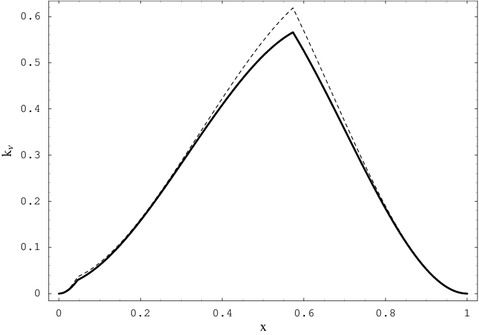
Presently there are various well developed codes - such as Pythia [25], SYBILL [27], QGSJET [35], DPMJET-III [28] - which implement different hadronic interaction models to study particle production in nucleon-nucleon or nucleon-nucleus collisions. It would be interesting to make a systematic comparison between the various codes, but this is beyond the scope of this work. In Ref.  [26], suitable parametrizations of the pion and kaon differential cross section in $pp$ collisions from the Pythia code are given. Moreover, parametrizations of $\pi^{0}$ and $\eta$ productions in $pp$ collisions, according SYBILL and QGSJET code, are presented in Ref.  [29]. In the left panel of Fig. 2, we use these parametrizations to calculate the relevant $f_{i}$ factors for $\alpha=2-4$. We see that the quantities $f_{i}$ are marginally dependent on the assumed spectral index and we take the values obtained for $\alpha=2$:

	$\displaystyle f_{\pi^{+}}=1.08\;\;\;$		$\displaystyle\;\;\;f_{\pi^{-}}=0.79\;\;\;\;\;\;\;\;\;\;\;\;f_{\eta}=0.48$
	$\displaystyle f_{K^{+}}=0.13\;\;\;$		$\displaystyle\;\;\;f_{K^{-}}=0.09$		(29)

as reference values in our calculations. We remark that, using these values, we improve on our previous calculation [16] where we assumed “isospin invariance” (i.e., $f_{\pi^{+}}=f_{\pi^{-}}=1$) and we overestimated the rate of $K^{\pm}$ production ($f_{K^{+}}=f_{K^{-}}=0.2$).

In order to estimate uncertainties in our method, we should compare the $f_{\rm i}$ factors in Eq. (29) with those obtained by using different hadronic interaction models. For assumed spectral index $\alpha=2$, the results of [30], which describes the various possible contribution to $\gamma$-production in $p$-ISM collisions, can be used to estimate the $f_{i}$ factors predicted by DPMJET-III. In this case, in fact, the factor $Z_{i}=\langle E_{i}\rangle/E_{\rm p}$ coincides with the average fraction of the parent particle energy carried by particles of the type $i$. This quantity can be related to the energy fraction emitted in photons, by taking into account the branching ratios and the kinematic of the decay processes. By using this approach, we estimate (when possible) the values presented in Tab. 1, where we also show the predictions obtained from Pythia and SYBILL parametrizations. We remark the Pythia and SYBILL results are obtained by assuming $pp$ collision, while the DMPJET-III results refer to the collision of protons with ISM, which is assumed to be composed by 90% protons, 10% helium nuclei, 0.02% carbon and 0.04% oxygen. One sees from Tab. 1 that there is a reasonable agreement between the prediction of the different codes. In particular, the $f_{i}$ factors are practically unchanged in the various cases. This means that the neutrino-photon ratio is a rather solid prediction, which should not suffer from large uncertainties in hadronic models and/or in the modelization of the CR flux and the ambient medium in the SNR.

Finally, we discuss the other assumptions in our approach. Our calculation neglects the contribution of $K^{0}_{S}$ and $K^{0}_{L}$ (and more rare production channels) to photon and neutrino production. According to Tab. 1, these processes accounts for several percents increase of the photon and neutrino production rates with compensating effects in the neutrino-photon ratio, which is affected at the few percents level. Moreover, we assumed that the ratio between the production rates of the various mesons does not depend on energy, nor on the CR spectral shape. This assumption is motivated by the “quasi-scaling” behavior of hadronic cross sections and by the results presented in Fig. 2 and it is valid with few percents accuracy. In conclusion, by taking into account the approximations implicit in our method (e.g., constant $f_{i}$ factors, neglected production channels, etc.), the uncertainties in hadronic modeling and the uncertainty in neutrino oscillation parameters, we can safely estimate that the neutrino fluxes predicted by our approach are accurate at the level of about 20%.⁵⁵ 5 As recalled in the Introduction, a possible limit of our (and other) calculations is the possible presence of a relevant leptonic contamination (component) of the gamma radiation, that requires efforts in theoretical modeling of the sources and multi-wavelength observations to be precisely assessed. Such a possibility implies that, conservatively, we should speak of an upper bound on the neutrino signal within the present information.

By using the $f_{i}$ factors given in Eq. (29) and the oscillation probabilities given in Eq. (21), one can calculate the photon-neutrino kernels $K^{\rm osc}_{\nu_{\mu}}[x]$ and $K^{\rm osc}_{\overline{\nu}_{\mu}}[x]$ according to Eqs. (19,20). Considering the explicit form of the the various contributions (see Eqs. (10,11)), one obtains the following simple analytic expression:

$$\Phi_{\nu_{\mu}}[E]=0.380\,\Phi_{\gamma}[E/(1-r_{\pi})]+0.0130\,\Phi_{\gamma}[E/(1-r_{K})]+\int_{0}^{1}\frac{dx}{x}\;k_{\nu_{\mu}}[x]\,\Phi_{\gamma}[E/x]$$

(30)

where the first two terms describe neutrinos produced in pions (first term) and kaons (second) decays. The kernel $k_{\nu_{\mu}}[x]$, which takes into account neutrinos produced by muon decay, is shown in the right panel of Fig. 2 and it is given by:

	$\displaystyle k_{\nu_{\mu}}[x]$	$\displaystyle=$	$\displaystyle x^{2}(15.34-28.93\,x)\;\;\;\;\;\;\;\;\;\;\;\;\;\;\;\;\;\;\;\;\;\;\;\;\;\;\;\;\;\;\;\;\;\;\;\;\;x\leq r_{K}=0.0458$		(31)
		$\displaystyle=$	$\displaystyle 0.0165+0.1193x+3.747x^{2}-3.981x^{3}\;\;\;\;\;\;\;\;r_{K}<x<r_{\pi}$
		$\displaystyle=$	$\displaystyle(1-x)^{2}\,(-0.6698+6.588x)\;\;\;\;\;\;\;\;\;\;\;\;\;\;\;\;\;\;\;\;\;\;\;\;x\geq r_{\pi}=0.573$

A similar relation holds for muon antineutrino flux:

$$\Phi_{\overline{\nu}_{\mu}}[E]=0.278\,\Phi_{\gamma}[E/(1-r_{\pi})]+0.0090\,\Phi_{\gamma}[E/(1-r_{K})]+\int_{0}^{1}\frac{dx}{x}\;k_{\overline{\nu}_{\mu}}[x]\,\Phi_{\gamma}[E/x]$$

(32)

where

	$\displaystyle k_{\overline{\nu}_{\mu}}[x]$	$\displaystyle=$	$\displaystyle x^{2}(18.48-25.33\,x)\;\;\;\;\;\;\;\;\;\;\;\;\;\;\;\;\;\;\;\;\;\;\;\;\;\;\;\;\;\;\;\;\;\;\;\;\;x\leq r_{K}=0.0458$		(33)
		$\displaystyle=$	$\displaystyle 0.0251+0.0826x+3.697x^{2}-3.548x^{3}\;\;\;\;\;\;\;\;r_{K}<x<r_{\pi}$
		$\displaystyle=$	$\displaystyle(1-x)^{2}\,(0.0351+5.864x)\;\;\;\;\;\;\;\;\;\;\;\;\;\;\;\;\;\;\;\;\;\;\;\;\;\;x\geq r_{\pi}=0.573$

Eqs. (30) and (32) have a general validity and do not require any specific parametrization of the photon spectrum. They will be used in the following to derive the neutrino flux from the SNR RXJ1713.7-3946 directly from the observational $\gamma-$ray data. It is, anyhow, interesting to discuss the application of these relations for the functional forms most commonly used to parametrize the photon spectrum.

Charged-current interactions of $\nu_{\mu}$ and $\overline{\nu}_{\mu}$ produce muons and antimuons that can be observed in neutrino telescopes. The number of muons and antimuons reaching an area $A$ and in a time of observation $T$ is:

$$N_{\mu+\overline{\mu}}=f_{\rm liv}\cdot A\cdot T\cdot\int_{E_{\rm th}}^{\infty}dE\;\Phi_{\nu_{\mu}}[E]\times Y_{\mu}[E,E_{\rm th}](1-\overline{a}_{\nu_{\mu}}[E])+(\nu_{\mu}\rightarrow\overline{\nu}_{\mu})$$

(46)

where $E$ is the energy of the neutrino at the point of interaction and $E_{\rm th}$ is the energy threshold for muon detection. Following [14]: (1) we assume $A=1{\rm km}^{2}$ and $T=1$ solar year; (2) we consider that the SNR RX J1713.7-3946 is visible for $f_{\rm liv}=78\%$ of the sideral year, as in Antares location; (3) the neutrino absorption coefficient $\overline{a}_{\nu_{\mu}}(E)$, averaged over the daily location of the source, is calculated for standard rock; (4) the probability $Y_{\mu}(E,E_{\rm th})$ that a neutrino of energy $E$ produce a muon that reach the detector with an energy larger than $E_{\rm th}$ is calculated for water.

The above equation can be rewritten in the form:

$$N_{\mu+\overline{\mu}}=\int_{E_{\rm th}}^{\infty}\frac{dE_{\nu}}{E_{\nu}}\;n_{\nu_{\mu}}[E_{\nu},E_{\rm th}]\;\Phi_{\nu_{\mu}}[E_{\nu}]+(\nu_{\mu}\rightarrow\overline{\nu}_{\mu})$$

(47)

where the function:

$$n_{\nu_{\mu}}[E_{\nu},E_{\rm th}]=f_{\rm liv}\cdot A\cdot T\cdot Y_{\mu}[E_{\nu},E_{\rm th}]\cdot(1-\overline{a}_{\nu_{\mu}}[E_{\nu}])\cdot E_{\nu}\\$$

(48)

gives the relative contribution of neutrinos with energy $E_{\nu}$ to the total event rate above a detection threshold $E_{\rm th}$. In the left panel of Fig. 5 we show the function $n_{\nu_{\mu}}[E_{\nu},E_{\rm th}]E_{\nu}^{-2.5}$ as a function of $E_{\nu}$ for the selected values $E_{\rm th}=0.05,\;0.2,\;1,\;5,\;20$ TeV. One sees that the bulk of the signal is expected to arise from the spectral region $E_{\nu}\simeq 0.3-100$ TeV which is directly constrained by photon observational data, provided that the detection threshold is below few TeV.

References

- [1] The modern formulation of the conjecture is in V.L. Ginzburg, S.I. Syrovatskii, Origin of Cosmic Rays (1964) Moscow, where it is noted that the losses of the Milky Way can be compensated if a fraction of the kinetic energy is accelerated into cosmic ray. The first suggestion to associate cosmic rays and supernovae was made in W. Baade, F. Zwicky, Proc. Natl. Acad. Sci. U.S.A. 20 (1934) 259, Phys. Rev. 46 (1934) 76.
- [2] C. Distefano, D. Guetta, E. Waxman and A. Levinson, Astrophys. J. 575 (2002) 378 [arXiv:astro-ph/0202200].
- [3] F. Halzen and D. Hooper, Rept. Prog. Phys. 65 (2002) 1025 [arXiv:astro-ph/0204527].
- [4] The original proposal is in E. Fermi, Phys. Rev. 75 (1949) 1169 and Astroph. J. 119 (1954) 1. The developments and subsequent implementations have been summarized in L.O’C. Drury et al., Space Sci. Rev. 99 (2001) 329; M.A. Malkov, L.O’C. Drury, Rep. Prog. in Physics 64 (2001) 429; A.M. Hillas, J. Phys. G, Nucl. Part. Phys. 31 (2005) R95; P. Blasi, Nucl. Instrum. Meth. A 588 (2008) 166.
- [5] V.S Berezinsky, S.V. Bulanov, V.A. Dogiel, V.L. Ginzburg (ed.), V.S. Ptuskin, Astrophysics of cosmic rays, (1990, Russian edition 1984) North Holland; V.S. Ptuskin, Origin of galactic cosmic rays: sources, acceleration, and propagation, Rapporteur talk at 29th ICRC (2005) 10, 317.
- [6] http://www.mpi-hd.mpg.de/hfm/HESS/HESS.html.
- [7] F. A. Aharonian [HESS Collaboration], Astrophys. J. 661 (2007) 236.
- [8] F. Aharonian [HESS Collaboration], Astron. Astrophys. 464 (2007) 235.
- [9] F. Aharonian [HESS Collaboration], Astron. Astrophys. 449 (2006) 223; E.G. Berezhko and H.J. Voelk, Astron. Astrophys. 451 (2006) 981; K. Moraitis and A. Mastichiadis, Astron. Astrophys. 462 (2007) 173.
- [10] B. Katz and E. Waxman, arXiv:0706.3485 [astro-ph].
- [11]
BAIKAL,
http://baikalweb.jinr.ru/;
AMANDA http://amanda.berkeley.edu
and http://nuastro-zeuthen.desy.de/e13/e43/index_eng.html;
IceCUBE, http://icecube.wisc.edu/
and http://nuastro-zeuthen.desy.de/e13/e14/index_eng.html;
ANTARES, http://antares.in2p3.fr/;
NEMO, http://nemoweb.lns.infn.it/project.htm;
NESTOR, http://www.nestor.org.gr/;
Km3NET, http://www.km3net.org/. - [12] T.K Gaisser, Cosmic rays and particle physics, (1990) Cambridge Univ. Press.
- [13] J. Alvarez-Muniz and F. Halzen, Astrophys. J. 576 (2002) L33 [arXiv:astro-ph/0205408].
- [14] M. L. Costantini and F. Vissani, Astropart. Phys. 23, 477 (2005) [arXiv:astro-ph/0411761].
- [15] V. Cavasinni, D. Grasso and L. Maccione, Astropart. Phys. 26 (2006) 41 [arXiv:astro-ph/0604004].
- [16] F. Vissani, Astropart. Phys. 26, 310 (2006) [arXiv:astro-ph/0607249].
- [17] F. Vissani, Vulcano Workshop 2006: Frontier Objects in Astrophysics and Particle Physics, Vulcano, Italy, 22-27 May 2006. Published in Vol. 93 of SIF Conference Proceedings edited by F. Giovannelli and G. Mannocchi, page 599, arXiv:astro-ph/0609575.
- [18] A. Kappes, J. Hinton, C. Stegmann and F. A. Aharonian, Astrophys. J. 656 (2007) 870 [arXiv:astro-ph/0607286].
- [19] M. D. Kistler and J. F. Beacom, Phys. Rev. D 74 (2006) 063007 [arXiv:astro-ph/0607082].
- [20] L. A. Anchordoqui, J. F. Beacom, H. Goldberg, S. Palomares-Ruiz and T. J. Weiler, Phys. Rev. D 75 (2007) 063001 [arXiv:astro-ph/0611581].
- [21] F. Vissani and F. L. Villante, Nucl. Instrum. Meth. A 588 (2008) 123.
- [22] F. L. Villante and F. Vissani, Phys. Rev. D 76, 125019 (2007) [arXiv:0707.0471 [astro-ph]].
- [23] P. Lipari as quoted in the caption of tab. 7.2 of [12]. See also L.V. Volkova, Proceedings of Erice 1988 Cosmic -rays, neutrinos and related astrophysics page 139 and S.M. Barr, T.K. Gaisser, P. Lipari and S. Tilav, Phys. Lett. B214 (1988) 147.
- [24] A. Strumia and F. Vissani, arXiv:hep-ph/0606054.
- [25] http://home.thep.lu.se/torbjorn/Pythia.html.
- [26] H. B. J. Koers, A. Pe’er and R. A. M. Wijers, arXiv:hep-ph/0611219.
- [27] R. S. Fletcher, T. K. Gaisser, P. Lipari and T. Stanev, Phys. Rev. D 50 (1994) 5710.
- [28] http://sroesler.web.cern.ch/sroesler/dpmjet3.html.
- [29] S. R. Kelner, F. A. Aharonian and V. V. Bugayov, Phys. Rev. D 74, 034018 (2006) [arXiv:astro-ph/0606058].
- [30] C. Y. Huang, S. E. Park, M. Pohl and C. D. Daniels, Astropart. Phys. 27 (2007) 429 [arXiv:astro-ph/0611854].
- [31] S. M. Bilenky and B. Pontecorvo, Phys. Rept. 41 (1978) 225.
- [32] G. L. Fogli, E. Lisi, A. Marrone, A. Palazzo and A. M. Rotunno, arXiv:0806.2649 [hep-ph] and references quoted therein.
- [33] J. G. Learned and S. Pakvasa, Astropart. Phys. 3 (1995) 267.
- [34] C. Y. Huang and M. Pohl, Astropart. Phys. 29 (2008) 282 [arXiv:0711.2528 [astro-ph]].
- [35] For a review, see S. Ostapchenko, AIP Conf. Proc. 928 (2007) 118 [arXiv:0706.3784 [hep-ph]].
- [36] P. Lipari, Nucl. Phys. Proc. Suppl. 175-176, 96 (2008).
- [37] P. Lipari, “Perspectives of high energy neutrino astronomy,” Nucl. Instrum. Meth. A 567 (2006) 405 [arXiv:astro-ph/0605535].