IPPP/08/52
DCPT/08/104
August 24, 2026
Diffractive dissociation re-visited for predictions at the LHC
E.G.S. Lunaa, V.A. Khozea,b, A.D. Martina and M.G. Ryskina,b
a Institute for Particle Physics Phenomenology, University of Durham, Durham, DH1 3LE
b Petersburg Nuclear Physics Institute, Gatchina, St. Petersburg, 188300, Russia
We describe the formalism, and present the results, for a triple-Regge analysis of the available and high-energy data which explicitly accounts for absorptive corrections. In particular, we allow for the gap survival probability, , in single proton diffractive dissociation. Since for scattering the value of is rather small, the triple-Pomeron vertex obtained in this analysis is larger than that obtained in the old analyses where the suppression caused by the absorptive corrections was implicitly included in an effective vertex. We show that the bare triple-Pomeron coupling that we extract from the and data is consistent with that obtained in a description of the HERA data. The analyses of the data prefer a zero slope, corresponding to the small size of the bare vertex, giving the hope of a smooth matching to the perturbative QCD treatment of the triple-Pomeron coupling.
1 Motivation
The total and elastic proton-proton cross sections are usually described in terms of an eikonal model [1]. The advantage of using an eikonal framework is that it automatically satisfies -channel unitarity, which follows once we include the elastic rescattering of the interacting particles. Furthermore, the Good-Walker formalism [2] allows the possibility of excited proton states occurring in the intermediate state. In this way we include low-mass diffractive dissociation. It was demonstrated in [3] that a two-channel eikonal is sufficient to capture the main features of this dissociation (provided, of course, we are not interested in the production of a particular resonant state), see also [4].
On the other hand, high-mass () diffractive dissociation is described in terms of the triple-Regge formalism, where the differential cross section, , is driven by the triple-Regge couplings . The values of these couplings were determined from the data available in triple-Regge domain in the 1970s; see, for example [5, 6, 7]. However, these early analyses did not allow for absorptive corrections, which are sizeable in hadron-hadron collisions. Therefore, the old triple-Regge couplings must be regarded, not as the bare vertices, but as effective couplings embodying absorptive effects. It was pointed out in Ref. [8] that the original bare triple-Pomeron vertex may be about three times larger than the effective coupling which is obtained with the neglect of absorptive corrections. However, absorptive effects are very sensitive to the -slope of the triple-Reggeon vertices and in the 1970s it was “impossible to determine the exact values of the bare triple-Pomeron coupling” [8]; the accuracy and energy range covered by the data were insufficient. So the results of the triple-Regge analyses were presented in the form of effective couplings. This leads to a problem, since the absorptive effects are not constant factors, but depend on the energy and the type of diffractive process. Since the inelastic cross section expected at the LHC is more than twice as large as that observed at fixed target and CERN-ISR energies, we cannot use the results of the old triple-Regge analyses to predict the diffractive effects at the LHC11 1 Already, in order to describe data up to the Tevatron energy, Goulianos and Montanha [9] found it necessary to restore unitarity by renormalising the “Pomeron flux” [10]. This mimics to some extent the absorptive effects.. It is therefore necessary to perform a new triple-Regge analysis that includes the absorptive effects explicitly. Here we present the first analysis of the available diffractive (and elastic) data in the CERN-ISR – Tevatron region in which the absorptive corrections are systematically included. The absorptive corrections are calculated in terms of a two-channel eikonal model fitted to describe the total and elastic differential cross section data for and scattering.
At the moment, the energy behaviour of the scattering amplitude may be consistently described by two different scenarios for the asymptotic regime [11]. One is called the weak coupling of the Pomerons. In this case, at very high energy, the cross sections tend to the universal constant value
| (1) |
In order not to violate unitarity, the triple-Pomeron coupling must vanish with vanishing transverse momentum transferred through the Pomeron [12]
| (2) |
Another possibility is called the strong coupling scenario [13]. Here, at a very high energies, the cross sections grows as
| (3) |
and the bare vertex
| (4) |
The present data are usually described within the Froissart-like limit of the second scenario (with ). However to reach asymptotics we need very high energy – the energy at which the slope of the elastic amplitude, is dominated by the second term, that is when . This is far beyond the energies available at present. Another possibility, to distinguish between the weak and strong approaches, is to study the dependence of the bare triple-Pomeron vertex. Thus, it is important to extract the bare vertex before its behaviour is affected by absorptive corrections.
This paper is devoted to a detailed analysis of “soft” scattering data using, in turn, the strong and weak triple-Pomeron coupling behaviours. In Section 2 we recall the Good-Walker formalism for the two-channel eikonal model, in Section 3 we briefly describe the parametrisation used to calculate the absorptive corrections for the triple-Reggeon cross sections and demonstrate that this parametrisation is consistent with the available data on the differential elastic () and total cross sections. Next, in Section 4, we give the formulae for the inclusive cross section, , in the triple-Regge region which incorporates the screening corrections caused by the two-channel eikonal. The results of our triple-Regge analyses of and data are presented in Section 5. We perform fits using both the strong and weak triple-Pomeron coupling. We find that the data favour the former ansatz. In Section 6 we discuss the description of the data for inelastic diffractive photoproduction, , obtained at HERA. We find that the HERA data again favour the strong triple-Pomeron coupling scenario. In Section 7 we present our conclusions.
2 Résumé of the eikonal formalism
2.1 Single-channel eikonal model
First, we briefly recall the relevant features of the single-channel eikonal model. That is we focus on elastic unitarity. Then “disc ” is simply the discontinuity of the scattering amplitude across the two-particle -channel cut. At high energies we have a sizeable inelastic component. The -channel unitarity relation is diagonal in the impact parameter, , basis, and may be written
| (5) |
with
| (6) | |||||
| (7) | |||||
| (8) |
These equations are satisfied by
| (9) | |||||
| (10) | |||||
| (11) |
where is called the opacity (optical density) or eikonal22 2 Sometimes is called the eikonal; for simplicity we omit the real part of . At high energies, the ratio is small, and can be evaluated via a dispersion relation.. From (11), we see that is the probability that no inelastic scattering occurs.
The opacity corresponding to an individual Regge pole or takes the form
| (12) |
where , and where the contribution to the amplitude from Reggeon exchange is33 3 Note that, unlike [3, 14, 15], here we use the normalisation , rather than . That is, as compared to our previous papers, here all the coupling constants ( and ) are decreased by a factor .
| (13) |
where the behaviour of the Reggeon-proton vertex is taken to have the exponential form
| (14) |
Thus, for a linear trajectory
| (15) |
the -slope of the amplitude is given by
| (16) |
For Regge exchange with signature , the factor in eq. (13) is
| (17) |
Although we take exponential forms for the exchange of the secondary Reggeons, we choose, as in Ref. [14], a power-like form for the proton-Pomeron vertex
| (18) |
Also, to improve the description of the low region, we follow Anselm and Gribov [16] and include pion-loop insertions44 4 Note that, in (20) below, we have corrected the misprint which occurs in the published version of [16]. in Pomeron exchange which results in a non-linear form of the Pomeron trajectory
| (19) |
where
| (20) |
with and GeV. The coefficient specifies the total cross section, and is the form factor of the pion-Pomeron vertex. The coefficient in (19) is small55 5 We use the additive quark model relation ., but due to the tiny scale the dependence of is steep and non-linear. It has an important effect on the local slope, , of the elastic cross section. For the results that we obtain below for the Pomeron trajectory, , it is important to note that expression (20) for has been renormalised [16], such that
| (21) |
where denotes the full pion-loop contribution. Further discussion of the pion-loop contribution can be found in Ref. [14].
Finally, the total opacity is given by the sum of all the allowed Regge exchanges
| (22) |
In the present simplified analysis we neglect the real part of the amplitude, since our goal is to investigate the role of the absorptive effect which is caused essentially by the imaginary part of the amplitude, that is by the real part of the opacity. Therefore, the values of the couplings , that we quote in Table 1 below, are actually , where the are the signature factors of (17).
2.2 Inclusion of low-mass diffractive dissociation
So much for elastic diffraction. Now we turn to inelastic diffraction, which is a consequence of the internal structure of hadrons. This is simplest to describe at high energies, where the lifetime of the fluctuations of a fast hadron is large, , and during these time intervals the corresponding Fock states can be considered as ‘frozen’. Each hadronic constituent can undergo scattering and thus destroy the coherence of the fluctuations. As a consequence, the outgoing superposition of states will be different from the incident particle, and will most likely contain multiparticle states, so we will have inelastic, as well as elastic, diffraction.
To discuss inelastic diffraction, it is convenient to follow Good and Walker [2], and to introduce states which diagonalize the matrix. Such eigenstates only undergo elastic scattering. Since there are no off-diagonal transitions,
| (23) |
a state cannot diffractively dissociate into a state . We have noted that this is not, in general, true for hadronic states, which are not eigenstates of the -matrix, that is of . To account for the internal structure of the hadronic states, we have to enlarge the set of intermediate states, from just the single elastic channel, and to introduce a multichannel eikonal. We will consider such an example below, but first let us express the cross section in terms of the probability amplitudes of the hadronic process proceeding via the various diffractive eigenstates66 6 The exponent exp describes the probability that the diffractive eigenstate is not absorbed in the interaction. Later we will see that the rapidity gap survival factors, , can be described in terms of such eikonal exponents. .
Let us denote the orthogonal matrix which diagonalizes by , so that
| (24) |
Now consider the diffractive dissociation of an arbitrary incoming state
| (25) |
The elastic scattering amplitude for this state satisfies
| (26) |
where and where the brackets of mean that we take the average of over the initial probability distribution of diffractive eigenstates. After the diffractive scattering described by , the final state will, in general, be a different superposition of eigenstates from that of , which was shown in (25). At high energies we may neglect the real parts of the diffractive amplitudes. Then, for cross sections at a given impact parameter , we have
| (27) | |||||
It follows that the cross section for the single diffractive dissociation of a proton,
| (28) |
is given by the statistical dispersion in the absorption probabilities of the diffractive eigenstates. Here the average is taken over the components of the incoming proton which dissociates. If the averages are taken over the components of both of the incoming particles, then in (28) we must introduce a second index on , that is , and sum over and . In this case the sum is the cross section for single and double dissociation.
3 Description of the elastic data
In preparation for the triple-Regge analysis of the data for high-mass diffraction, we first perform a two-channel eikonal fit to all the high-energy and total cross section data above GeV and to the elastic differential scattering cross section for at , 53 and 62 GeV, and for at , 53, 62, 546 and 1800 GeV. We use total cross section data sets compiled by the Particle Data Group [17] and differential cross section data sets from the references [18] (ISR), [19] () and [20] (Tevatron), see the review in Ref. [21]. The statistic and systematic errors of all scattering quantities have been added in quadrature.
We introduce a parameter to define the two diffractive eigenstates of the eikonal model, such that their couplings to the Pomeron are
| (29) |
where the proton wave function , see Ref. [14]. The CERN-ISR measurements of the excitations into particular channels ( etc.) with GeV [22] correspond to a cross section for low-mass diffraction of77 7 Here, and in what follows, the value of accounts for dissociation of both colliding particles.
| (30) |
This value corresponds to , which we take in this analysis.
We describe the and total and elastic cross section data in terms of Pomeron, and positive () and negative () signature Regge exchange. The positive signature secondary Reggeons, and , are taken to lie on an exchange-degenerate linear trajectory with intercept and coupling88 8 If we assume the additive-quark-model relation, , then the coupling . to the proton of parametric form
| (31) |
see (14). Similarly, the exchange-degenerate negative signature pair () are described by parameters and . The slopes, , of the secondary Reggeon linear trajectories are fixed at 0.9 . On the other hand, the Pomeron coupling and trajectory are taken to have parametric forms given by (18) and (19), respectively.
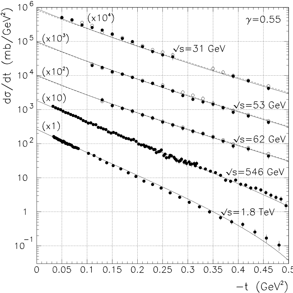
The values of the Regge parameters determined by the global fit are listed in Table 1. The fit has . The description of and is displayed in Fig. 1, where the solid (dashed) curves correspond to () scattering. The total cross section at LHC is predicted99 9 As expected, the inclusion of absorption reduces the value of the cross section predicted at the LHC energy. Indeed, if the high-mass diffractive absorptive effects were also included then the total cross section would be further reduced to about 90 mb [3, 23], see also [24, 4]. The present model also predicts an elastic differential cross section at the LHC energy with a diffractive dip at . However, for this prediction to be reliable we must await the inclusion of the high-mass absorptive effects in the elastic analysis [23]. An earlier analysis [3], which included high-mass diffraction phenomenologically, showed that, at the LHC energy, the dip occurred at larger and that the elastic cross section was smooth in the region shown in Fig. 1. to be mb.

4 High-mass diffraction: triple-Regge formalism
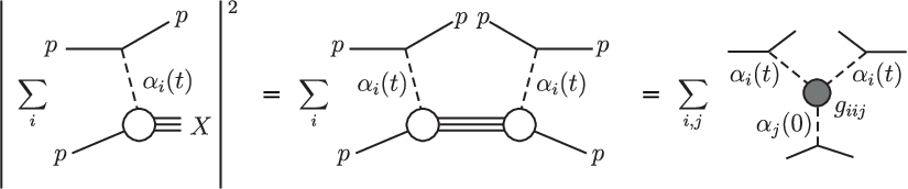
The multichannel eikonal is unable to account for diffraction into high mass states. These processes, with large , are usually described in terms of a triple-Regge formalism, where
| (32) |
where is the momentum fraction of the ingoing proton carried by the outgoing proton. The approach is sketched in Fig. 2. Since we have large we no longer have . Rather, we must allow for non-vanishing
| (33) |
To the best of our knowledge, the screening corrections have not been explicitly included in the triple-Regge formalism. Therefore we present the formalism below, first using a single-channel eikonal and then generalising it to the two-channel case. Finally we treat the corrections to the diagram as a special case.
4.1 Screening corrections in the triple-Regge formalism

If we first neglect the screening correction, then the triple-Regge diagram of Fig. 2 gives the contribution
| (34) |
We use a simple exponential parametrisation of the triple-Regge vertices
| (35) |
where the momenta are defined in Fig. 3, and where .
Screening effects are best included by working in impact parameter space and using suppression factors of the form exp(). To determine the or dependence we take the Fourier transforms with respect to the impact parameters specified in Fig. 3. We obtain1010 10 Note that as .
| (36) |
where
| (37) |
| (38) |
and where the -independent factors are collected in
| (39) |
These equations assume that we have a strong triple-Pomeron scenario, see (4). For the weak triple-Pomeron coupling ansatz, (2), we must include a factor in the integrand of the expression (37) for when , and also in the analogous formula for .
To include the screening corrections, for a single-channel eikonal, we must include in the integrands on the right-hand side of (36) the factors
| (40) |
That is, we need to compute
| (41) |
where is given by
| (42) |
4.2 Generalisation to a two-channel eikonal
Recall that in the two-channel eikonal, we take the Pomeron couplings to each diffractive eigen component to be1111 11 Following [14], we assume the same structure, that is the same shape and size for each component, apart, of course, from the cross section.
| (43) |
On the other hand, for the secondary Reggeons, , which are believed to dominantly couple to valence quarks, we take
| (44) |
that is, the same for each component. Thus for the , and couplings (with ) we make the replacement
| (45) |
in (41), whereas for the and (with ) we let
| (46) |
The subscripts are used to denote the eigen components respectively. In addition for we replace , with , in (42) by
| (47) |
and for
| (48) |
These replacements of are for the and contributions. For the and contributions, with or , we have
| (49) |
| (50) |
4.3 The screening of the contribution
We treat the contribution as a special case due to the presence of the spin-flip amplitude. First, neglecting screening, we have
| (51) |
where [25]. Since the pion is almost on-mass-shell, we expect , according to the additive quark model. In other words
| (52) |
The factor in (51) is given by
| (53) |
where the term is of proton spin-flip (sf) origin, and the remaining two terms are spin non-flip. Here, is the Pauli matrix associated with the spin of the incoming proton. The non-flip interaction, is screened in the usual way, see (45), (49) and (50). However, the spin-flip amplitude is now a vector directed along . Thus the integrals in (37) and (42) should be written in vector form, with
| (54) |
and in (39) replaced by . This leads to
| (55) |
and
| (56) |
with directed along . After the azimuthal integration, it means that the Bessel function , that arises in (37), should be replaced by .
5 Triple-Regge analysis of and data
The main objective of this paper is to perform a triple-Regge analysis of the available data for and (where ), allowing for screening (that is absorptive) effects. In this way we obtain a more reliable estimate of the bare triple-Pomeron coupling, , which is a vital ingredient in the description of diffractive processes at high energy, see Ref. [12, 13, 26]. As can be seen from the triple-Regge formalism of the previous section, it is necessary to work in impact parameter space in order to include screening corrections. However, it is computationally time-consuming to evaluate the required Fourier transforms inside a fit. To facilitate the fit to the data, we therefore first prepare grids of the integral in (41) for a range of fixed values of the slopes of the triple-Regge vertices for each and data point. A MINUIT fit to the data is then performed using Chebyshev polynomial interpolation in .
In fact, we performed three triple-Regge fits to the data with different assumptions for the form of the triple-Pomeron vertex. The first two assume either a strong or weak coupling triple-Pomeron vertex, that is they correspond to
| (57) |
respectively, see (4) and (2); recall that we use GeV units. The third fit considers a combination of the two couplings with both and as free parameters.
We fit to CERN-ISR1212 12 We choose a subset of the ISR data which is sufficient to fully describe their and dependence. [27], FNAL fixed-target [28] and Tevatron [29] data for and . The differential distributions for the FNAL fixed target and Tevatron experiments can be found in Ref. [9]. The relative normalisations of the data sets are not very well known. In Ref. [9] it was claimed that the normalisation uncertainties of the FNAL data are about 10. We fix the normalisation of the ISR data and introduce normalisation factors for the FNAL data with a 10 error. However, we find that the Tevatron data prefer to be normalised up by the strong coupling fit, and down for the weak coupling fit, by factors of about 25. We restrict this freedom and limit the normalisation factors to and for and 1800 GeV data respectively, where the and signs refer to the strong and weak coupling fits respectively. The remaining normalisations coming from the fits are for the GeV data [28].
All three fits to the data prefer very small, or even negative, slopes, , of the triple-Regge vertices. To avoid unphysical negative slopes, we impose the condition that . In fact, the optimum for each fit has, within error bars, all . Therefore, for the couplings quoted in Table 2, we have set all the slopes . The only exceptions to this are the slopes of the and vertices for the weak coupling fit, which are found to be positive, as shown in Table 2. We fixed the triple coupling at the additive quark model value, . Actually the data prefer a smaller value, but with a large error. However the fixed value of only enlarges by less than 0.5. The couplings of the Reggeons to the proton are taken from the “elastic” analysis of Section 3. The values of the remaining parameters, corresponding to the optimum triple-Regge fits, are given in Table 2.
| strong | weak | combination | |
| - | |||
| - | |||
| - | - | ||
| - | - | ||
| /DoF | 0.83 | 1.40 | 0.83 |
We see from the per degree of freedom (DoF) that the data clearly prefer the strong, rather than the weak, triple-Pomeron coupling ansatz. This is also clear from the ‘‘weak+strong combination’’ fit, which is dominated by the strong coupling component, and is little changed from the pure strong coupling fit1313 13 The normalisations of the data that are found in the “combination” fit are the same as those of the strong coupling fit.. The preference for the strong triple-Pomeron coupling is also evident from Fig. 4. This compares the “strong” and “weak” descriptions of a sample of the data that are fitted, including especially the high energy FNAL data at 546 and 1800 GeV. The FNAL data are most relevant since the triple-Pomeron contribution dominates for . We see that the weak coupling description of the shape of these data is disfavoured.

The -dependence of the single diffractive cross section, , is shown, for example, in Fig. 5 for at GeV, and in Fig. 6 for at the much lower energy corresponding to . We also show the individual triple-Regge contributions in these plots, together with the data available at these kinematic values. Note that, after accounting for the absorptive effects, the triple-Pomeron contribution does not vanish in the forward direction even in the weak coupling fit. Therefore to choose between the weak and strong coupling scenarios we have had to perform a full fit of the data. It is not enough just to study the low behaviour of the cross section. The first indication of the weak coupling characteristics is seen in Fig. 5 for and at the Tevatron energy. In this domain the data favour the strong coupling scenario. For larger values of the dip produced by the term in the weak coupling case is filled in by the peak due to the term. At the lower energy, corresponding to 550 , we see, from Fig. 6, that it is difficult to distinguish between the two scenarios. However, at the higher energy of the LHC the weak coupling scenario will reveal itself by a well pronounced dip at after which increases with up to , see Fig. 7. It is clear from Fig. 7 that single diffractive dissociation data obtained at the LHC for should be able to readily distinguish between the strong and weak triple-Pomeron coupling scenarios.


In the remainder of this Section, we discuss only the favoured strong triple-Pomeron coupling fit, for which the triple-Regge couplings are the first set listed in Table 2. The values of these couplings are rather stable. They never go outside the quoted errors when we change the renormalisation parameters of the data, or allow to be a free parameter. The quality of the fit is excellent, with a minimum . The 8 parameters are the 4 couplings, , and the 4 data renormalisations. The quality of the description can been seen from the plots of samples of the data that are fitted, Fig. 8 and Fig. 9, which also show the various triple-Regge contributions to the cross section.


In comparison with the old triple-Regge analysis of Ref. [6], we now obtain a more than twice larger relative contribution of the term. This is mainly due to the inclusion in our analysis of the higher energy Tevatron data. The inclusive cross sections measured in the interval of at the Tevatron energies turn out to be about twice smaller than that measured at the low CERN-ISR energies.
The “strong coupling” parameters of Table 2 are much closer to the bare triple-Reggeon couplings than those coming from the old fits [5, 6, 7] which did not allow for the screening corrections. In particular the value1414 14 Note that this result is in reasonable agreement with the parametrisation of the renormalised triple-Pomeron amplitude of Ref. [9] which leads to .
| (58) |
is consistent with the reasonable extrapolation of the perturbative BFKL Pomeron vertex to the low scale region [30]. However, these are still not the true bare vertices. For these sizeable values of the effect of “enhanced” screening, shown in Fig. 10, is not

negligible. Moreover, it is not enough to just take one iteration, that is, to repeat the ‘‘elastic’’ analysis, but now including the effects of the triple-Regge high-mass absorption, obtain new Regge-proton parameters and then repeat the triple-Regge analysis1515 15 Note that an eikonal-type model for absorption will still violate -channel unitarity [31]. At large , on the periphery, where the opacity is small, the effect of eikonal screening is not effective. For these (large ) partial waves the contribution coming from diffractive dissociation becomes larger than the total inelastic contribution. To satisfy unitarity more complicated (enhanced) multi-Pomeron diagrams must be included.. Rather, it is necessary to sum up the series of multi-Reggeon diagrams. We have considered such a model [23], that is an extension of an earlier model [3] but now including non-zero as a free parameter, as well as more -channel exchanges. The tuning of this model shows that it is possible to obtain a good description of the data provided that the triple-Pomeron coupling is a bit larger
| (59) |
6 Inelastic photoproduction
In Ref. [26] it was pointed out that the observation of the process at large values of offers, in principle, an opportunity to determine the triple-Pomeron coupling where the screening corrections are smaller than in the pure hadronic reactions, see also [32]. Unfortunately, the distribution has not been measured yet. However there exists a comparison of the HERA data for the “elastic” photoproduction process, with the proton dissociation data. The ratio, at the photon-proton centre-of-mass energy GeV and , is [33]-[37].
| (60) |
where the “inelastic” cross section has been integrated over the mass region GeV. Since only the Pomeron couples to charm quarks, the ratio is described by the and contributions. The cross section for absorption is rather small. So we may neglect the screening factor, and obtain
| (61) |

Note that the Pomeron trajectories and in (61), that is in the triple-Pomeron diagram in Fig. 11, are not the same. The lower Pomeron in Fig. 11 is the usual ‘soft’ Pomeron; whereas the upper ones, with , include DGLAP evolution from a low initial scale up to a rather large scale at the production vertex. The summation of the double logarithms leads to a steeper -dependence and hence to a larger effective intercept for the trajectory of the upper ‘hard’ Pomeron. Thus to evaluate the ratio of (61) we take , which corresponds to the dependence observed in the HERA data [34]-[37]. Taking the other parameters from Table 1 and the strong coupling fit of Table 2, we obtain for the two terms in (61)
| (62) |
This is consistent with the HERA data, within the uncertainties.
We also use the weak triple-Pomeron coupling fit of Table 2 to evaluate the ratio at . This is the lowest value for which is measured. The experimental value is1616 16 The measured ratio at is larger than that of (60) at , since the cross section of the elastic process, , has a larger -slope than that for . [33]
| (63) |
When we evaluate the weak coupling and contributions to , we find
| (64) |
a value about a factor two smaller than that observed. So again the strong triple-Pomeron coupling is favoured over the weak.
Originally, the strong triple-Pomeron coupling was supported by an analysis [26] of the HERA photoproduction data. The problem is that, at present, the dependence of the cross section has not been measured; only the value integrated over an interval is given. The large value of the triple-Pomeron coupling that was extracted in [26] assumed that the whole cross section originates from Pomeron exchange, and neglected the secondary Reggeon contribution. Here we have included the secondary Reggeon contribution. However, if the distribution were to be observed, it would then be possible to separate these contributions using just the photoproduction data, and to give an independent check of the results of our triple-Regge analysis. Clearly a dedicated measurement of the process , including especially the and dependence, would be extremely informative.
7 Conclusions
We have performed a triple-Regge analysis of the available and data, in which we account for absorptive effects. Thus, the couplings of the triple-Reggeon vertices extracted in this analysis will be much closer to the couplings of the original bare vertices than those obtained in the old analyses, where the screening corrections were implicitly included in the values of effective couplings.
The triple-Pomeron vertex turns out to be rather large, . This indicates that, in a more precise description of “soft” interactions, we must include more complicated ’enhanced’ diagrams and diagrams with the multi-Pomeron vertices (that is with a larger number of Pomerons in a vertex).
Due to the inclusion of the high-energy Tevatron data in the analysis, we now obtain a twice larger relative contribution of the term in comparison with the results of the old analyses.
We considered two possible parametrisations of the small behaviour of the triple-Pomeron vertex:
| (65) |
in GeV units. We found that the data prefer the first, the so-called strong Pomeron coupling scenario. In the second, the so-called weak coupling, case, we obtained a much poorer description of the high-energy Tevatron (CDF) data at small and low GeV2, where the triple-Pomeron contribution dominates. It will be important to measure the inclusive cross section for single diffraction, , at the LHC to confirm this conclusion. This could be done when the forward detectors are operating at the LHC, even at moderate integrated luminosity [38]. Another possibility is to study in more detail diffractive production with dissociation of the target proton. That is, to measure the and dependence of the reaction. The HERA experiments have so far only presented the cross section integrated over up to GeV. However, already these data support the strong coupling solution.
Finally, we note that our analysis of the data prefers zero slopes, corresponding to small size of the bare triple-Reggeon vertices. Together with the larger values of the and vertices, this gives hope that there is a smooth matching to the perturbative QCD treatment of the Pomeron.
Acknowledgements
We thank Aliosha Kaidalov, Alessia Bruni and Risto Orava for useful discussions. MGR and EGSL thank the IPPP at the University of Durham for hospitality. The work was supported by INTAS grant 05-103-7515, by grant RFBR 07-02-00023, by the Russian State grant RSGSS-3628.2008.2 and by the CNPq (Brazil) under contract 210242/2006-0.
References
- [1] for a recent review see M. M. Block, Phys. Rept. 436, 71 (2006).
- [2]
M.L. Good and W.D. Walker, Phys. Rev. 120 (1960) 1857;
E.L. Feinberg and I.Ya. Pomeranchuk, Doklady Akad. Nauk SSSR 93 (1953) 439; Suppl. Nuovo Cimento v. III, serie X, (1956) 652. - [3] M.G. Ryskin, A.D. Martin and V.A. Khoze, Eur. Phys. J. C54 (2008) 199.
- [4] E. Gotsman, E. Levin, U. Maor and J. S. Miller, arXiv:0805.2799 [hep-ph] and references therein.
- [5]
A.B. Kaidalov, V.A. Khoze, Yu.F. Pirogov and N.L. Ter-Isaakyan, Phys.
Lett. B45 (1973) 493;
A.B. Kaidalov and K.A. Ter-Martirosyan, Nucl. Phys. B75 (1974) 471. - [6] R.D. Field and G.C. Fox, Nucl. Phys. B80 (1974) 367.
- [7] for a review see A.B. Kaidalov, Phys. Rep. 50 (1979) 157.
- [8] A. Capella, J. Kaplan and J. Tran Thanh Van, Nucl. Phys. B105 (1976) 333.
- [9] K. Goulianos and J. Montanha, Phys. Rev. D59 (1999) 114017.
- [10] K. Goulianos, Phys. Lett. B358 (1995) 379; arXiv:hep-ph/9502356.
- [11] M.G. Ryskin, A.D. Martin and V.A. Khoze, in Proc. of Gribov Memorial Workshop (Budapest, May 2005), p. 115, arXiv:hep-ph/0506272.
- [12]
V.N. Gribov and A.A. Migdal, Sov. J. Nucl. Phys. 8 (1969) 583;
V.N. Gribov, Sov. J. Nucl. Phys. 17 (1973) 313. - [13] V.N. Gribov and A.A. Migdal, Sov. Phys. JETP 28 (1969) 784.
- [14] V.A. Khoze, A.D. Martin and M.G. Ryskin, Eur. Phys. J. C18 (2000) 167.
- [15] A.B. Kaidalov, V.A. Khoze, A.D. Martin and M.G. Ryskin, Eur. Phys. J. C21 (2001) 521.
- [16] A.A. Anselm and V.N. Gribov, Phys. Lett. B40 (1972) 487.
- [17] W.-M. Yao et al., J. Phys. G33, 1 (2006).
- [18] A. Breakstone et al., Nucl. Phys. B248, 253 (1984).
- [19] M. Bozzo et al., Phys. Lett. B147, 385 (1984).
- [20] N.A. Amos et al., Phys. Lett. B247, 127 (1990).
- [21] K. Goulianos, Phys. Rept. 101 (1983) 169.
- [22]
L. Baksay et al., Phys. Lett. B53 (1975) 484;
R. Webb et al., Phys. Lett. B55 (1975) 331;
L. Baksay et al., Phys. Lett. B61 (1976) 405;
H. de Kerret et al., Phys. Lett. B63 (1976) 477;
G.C. Mantovani et al., Phys. Lett. B64 (1976) 471. - [23] V.A. Khoze, A.D. Martin and M.G. Ryskin, in preparation.
- [24] S. Sapeta and K.J. Golec-Biernat, Phys. Lett. B613 (2005) 154.
- [25]
V. Stoks, R. Timmermans and J.J. de Swart, Phys. Rev.
C47 (1993) 512;
R.A. Arndt, I.I. Strakovsky, R.L. Workman and M.M. Pavan, Phys. Rev. C52 (1995) 2120. - [26] V.A. Khoze, A.D. Martin and M.G. Ryskin, Phys. Lett. B643 (2006) 93.
- [27] J.C.M. Armitage et al., Nucl. Phys. B194 (1982) 365.
- [28] R.L. Cool et al., Phys. Rev. Lett. 47 (1981) 701.
- [29] F. Abe et al., Phys. Rev. D50 (1994) 5535.
- [30] J. Bartels, M.G. Ryskin and G.P. Vacca, Eur. Phys. J. C27 (2003) 101.
- [31] E.S. Martynov and V.S. Struminsky, Phys. Atom. Nucl 59 (1996) 1755.
- [32] E. Gotsman, A. Kormilitzin, E. Levin and U. Maor, Eur. Phys. J. C52, 295 (2007).
- [33] ZEUS collaboration: Abstract 549, Int. Europhysics Conf. on HEP, Aachen, July 2003.
- [34] ZEUS collaboration: S. Chekanov et al., Nucl. Phys. B695 (2004) 3.
- [35] H1 collaboration: C. Adloff et al., Eur. Phys. J. C10 (1999) 373.
- [36] ZEUS collaboration: S. Chekanov et al., Eur. Phys. J. C24 (2002) 345.
- [37] H1 collaboration: A. Aktas et. al., Eur. Phys. J. C46 (2006) 585.
- [38] V.A. Khoze, A.D. Martin and M.G. Ryskin, Eur. Phys. J. C55 (2008) 363.