Exclusive ${\bf b\rightarrow s(d)\ell\ell}$ Decays

The flavor-changing neutral-current (FCNC) processes, $b\rightarrow s(d)\ell\ell$, provide an interesting hunting ground to look for new-physics phenomena. In the Standard Model (SM), FCNC transitions are forbidden at tree level, but they are allowed to proceed via electroweak-loop and weak-box diagrams. Lowest-order processes are depicted in Figure 1. The electroweak loops consist of a W-boson and a $t,~c$ or $u$-quark, where the $t$-quark contribution dominates. One of the loop particles radiates a photon or Z-boson to conserve momentum. In the weak-box diagram the $b$ to $s(d)$ transition occurs via the emission of two $W$ bosons. The emitted lepton pair is $e^{+}e^{-}$, $\mu^{+}\mu^{-}$, $\tau^{+}\tau^{-}$, or $\nu\bar{\nu}$. Final states with a $\tau^{+}\tau^{-}$ pair, however, are difficult to measure because of the missing neutrinos and are not discussed further.

In chapter 2, we discuss properties of the exclusive decays $B\rightarrow K^{(*)}\ell^{+}\ell^{-}$ where $\ell^{+}\ell^{-}$ is either $e^{+}e^{-}$ or $\mu^{+}\mu^{-}$ and introduce the observables we measure. In chapter 3, we focus on BABAR measurements of $B\rightarrow K^{(*)}\ell^{+}\ell^{-}$ branching fractions, isospin asymmetries, direct $C\!P$ violation and lepton flavor universality after discussing the analysis strategy. In chapter 4, we discuss the BABAR angular analysis of $B\rightarrow K^{*}\ell^{+}\ell^{-}$ decays. In chapter 5, we present the latest branching fraction upper limits of $B\rightarrow\pi\ell^{+}\ell^{-}$ decays. In chapter 6, we show results of recent searches for $B\rightarrow K\nu\bar{\nu}$ and $B\rightarrow K^{*}\nu\bar{\nu}$ before concluding in chapter 7.

The SM calculations are based on a low-energy effective Hamiltonian [1] that factorizes perturbatively-calculable short-distance contributions expressed by Wilson coefficients, $C_{i}$, from the non-perturbative long-distance contributions of the $b\rightarrow s$ transition operators, ${\cal O}_{i}$. In lowest order, dominant contributions result from the magnetic dipole operator ${\cal O}_{7}$, the vector-current operator ${\cal O}_{9}$ and the axial-vector-current operator ${\cal O}_{10}$. While ${\cal O}_{7}$ represents the photon penguin diagram, ${\cal O}_{9}$ and ${\cal O}_{10}$ result from linear combinations of the weak penguin and weak box diagrams. Thus, the relevant Wilson coefficients for these modes are $C_{7}$, $C_{9}$ and $C_{10}$. QCD effects, however, introduce operator mixing. Besides $\alpha_{s}$ corrections, the Wilson coefficients also receive contributions from other operators [2, 3, 4]. It is customary to absorb these by defining effective Wilson coefficients $\widetilde{C}_{i}$. The Wilson coefficients are functions of the renormalization scale $\mu$ and the squared dilepton mass, $q^{2}$. For low values of $q^{2}$, $\rm\mu=4.6~GeV$ and a top quark mass $\widehat{m}_{t}(\widehat{m}_{t})=167~\rm GeV/c^{2}$ in the $\overline{MS}$ renormalization scheme, the SM predictions at next-to-next-to-leading order (NNLO) yield $\widetilde{C}_{7}=-0.31$, $\widetilde{C}_{9}=4.21$ and $\widetilde{C}_{10}=-4.31$ [5, 2, 3]. The magnitude of $\widetilde{C}_{7}$ is constrained experimentally by ${\cal B}(B\rightarrow X_{s}\gamma)$ [6].

Since FCNC transitions are suppressed in the SM, loops and box diagrams from processes beyond the SM may yield non-negligible contributions. For example, new contributions may arise from loops containing a charged Higgs boson or supersymmetric (SUSY) particles [7, 8, 9]. Examples are shown in Figure 2. New physics contributions will modify the effective Wilson coefficients from their SM expectations. In addition, scalar and pseudoscalar couplings that are absent in the SM may modify the decay rate [4]. In order to have the ability for uncovering new physics phenomena, the SM predictions need to have sufficient precision. Most recent calculations use QCD factorization to separate the short-distance physics from the long-distance effects [5, 10]. The effective Wilson coefficients entering the short-distance part are calculated in the NNLO approximation. The long-distance effects including the hadronization process are expressed in terms of hadronic matrix elements of the $b\rightarrow s$ transition operators between the initial $B$ and the $K^{(*)}$ final states. Since the hadronic matrix elements cannot be calculated from first principles, they are parameterized in terms of form factors [11] that are calculated with the help of light-cone sum rules (LCSR) [12] or in soft-collinear effective theory (SCET) [13]. Though the form-factor calculations include next-to-leading order (NLO) QCD corrections they bear large theoretical uncertainties that are presently the dominant uncertainties in the SM predictions for exclusive decays. Thus, it is important to measure many different observables in different inclusive and exclusive electroweak penguin processes in order to extract meaningful results for moduli and arguments of the effective Wilson coefficients.

Figure 3 shows the $q^{2}$ dependence of the $B\rightarrow K^{*}\ell^{+}\ell^{-}$ branching fraction in the SM [11]. The overall shape is determined by the $q^{2}$ dependence of $\widetilde{C}_{9}(q^{2})$ except for the low $q^{2}$ region that is dominated by the $1/q^{2}$ term originating from $B\rightarrow K^{*}\gamma$. The singularity at $q^{2}=0$, which is not present in $B\rightarrow K\ell^{+}\ell^{-}$, is cut off by the finite $m_{\ell}$ masses. Thus, ${\cal B}(B\rightarrow K^{*}e^{+}e^{-})$ is expected to be $\sim 25\%$ larger in the SM than ${\cal B}(B\rightarrow K^{*}\mu^{+}\mu^{-})$, where the increase in branching fraction comes just from the extended $q^{2}<4m_{\mu}^{2}$ region. In addition, the hadronic decays $B\rightarrow J/\psi K^{*}$ and $B\rightarrow\psi(2S)K^{*}$ with $J/\psi,\psi(2S)\rightarrow\ell^{+}\ell^{-}$ interfere with signal modes. Since the branching fractions of the charmonium modes are more than two orders of magnitude larger than those of signal modes, we need to exclude sufficiently large $q^{2}$ regions in the vicinity of the charmonium resonances to remove them (see section III).

Besides partial and total branching fractions, asymmetries are of great interest in testing the SM, in particular for exclusive decays since many uncertainties in both predictions and measurements cancel [14]. For $B\rightarrow K\ell^{+}\ell^{-}$ and $B\rightarrow K^{*}\ell^{+}\ell^{-}$ we have performed new measurements of the isospin asymmetries, direct $C\!P$ violation and lepton flavor universality.

The $C\!P$-averaged isospin asymmetry is defined as

Besides $q^{2}$, the $B\rightarrow K^{*}\ell^{+}\ell^{-}$ differential decay rate also depends on three angles, $\theta_{K},\theta_{\ell}$, and $\chi$, where $\theta_{K}$ is the angle between the $K$ and the $B$ momenta in the $K^{*}$ rest frame, $\theta_{\ell}$ is the angle between the $\ell^{+}(\ell^{-})$ and the $B(\bar{B})$ momentum in the $\ell^{+}\ell^{-}$ rest frame, and $\chi$ is the angle between the $K^{*}$ and $\ell^{+}\ell^{-}$ decay planes. The present data sample is not large enough to perform a full three-dimensional angular analysis. Thus, we fit the one-dimensional angular distributions [16]

The parameter ${\cal F}_{L}$ is the $K^{*}$ longitudinal polarization. The second parameter, ${\cal A}_{FB}$, is the lepton forward-backward asymmetry. Both parameters are functions of $q^{2}$. Figures 5 shows the $q^{2}$ dependence of the $K^{*}$ longitudinal polarization. In addition to the SM prediction, the distribution for the flipped-sign $\widetilde{C}_{7}$ model is shown for which the sign of $\widetilde{C}_{7}$ is opposite to that in the SM.

The $q^{2}$ dependence of lepton forward-backward asymmetry is given by

The functions $A_{1}(q^{2}),V(q^{2}),T_{1}(q^{2})$ and $T_{2}(q^{2})$ are $q^{2}$-dependent form factors. The shape of the lepton forward-backward asymmetry results from different $q^{2}$ dependences of the interference terms $-\widetilde{C}_{9}(q^{2})\widetilde{C}_{10}(q^{2})$ and $-\widetilde{C}_{7}(q^{2})\widetilde{C}_{10}(q^{2})/q^{2}$. In the SM, the first (second) term is positive (negative) and increases (decreases) with $q^{2}$. Thus, ${\cal A}_{FB}$ is negative at low $q^{2}$, crosses zero and remains positive for large values of $q^{2}$ [11, 16, 18]. For $B\rightarrow K^{*}\ell^{+}\ell^{-}$ the zero crossing is predicted in NLO at $q^{2}_{0}=4.2\pm 0.6$. Figure 6 shows the low $q^{2}$ region for $B\rightarrow K^{*}\ell^{+}\ell^{-}$ [8]. The uncertainty of $q^{2}_{0}$ is dominated by uncertainties in the form-factor calculations. This is different for inclusive modes. Recent calculations of ${\cal A}_{FB}$ in $B\rightarrow X_{s}\ell^{+}\ell^{-}$ at order ${\cal O}(\alpha^{2}_{s})$ (NNLO) that include in addition electromagnetic corrections predict a $q^{2}$ dependence shown in Figure 7 [19]. The zero crossing is expected at $q^{2}_{0}=3.5\pm 0.12$.

Figure 8 shows the SM prediction of ${\cal A}_{FB}(q^{2})$ in the entire $q^{2}$ region. New physics may change both magnitude and phase of the Wilson coefficients [20] yielding shapes that differ from those in the SM. We consider three simple examples, also shown in Figure 8, in which the signs of the two interference terms are reversed ($i.e.$ a phase change by $\pi$) [11, 14, 16, 22, 21, 23, 24]. Changing the sign in $\widetilde{C}_{7}$, yields a positive ${\cal A}_{FB}$ for all values of $q^{2}$, whereas a reversed sign in $\widetilde{C}_{9}(q^{2})\widetilde{C}_{10}(q^{2})$ yields a negative ${\cal A}_{FB}$ in the entire $q^{2}$ region. If the sign of both interference terms is flipped, the resulting distribution has the negative mirror image of the SM distribution.

We have studied the exclusive decays $B\rightarrow K\ell^{+}\ell^{-}$ and $B\rightarrow K^{*}\ell^{+}\ell^{-}$ using $384$ million $B\kern 1.79993pt\overline{\kern-1.79993ptB}{}$ pairs collected at the $\mathchar 28935\relax{(4S)}$ resonance with the BABAR detector [25] at the PEP-II asymmetric-energy $e^{+}e^{-}$ collider. We reconstruct ten individual final states, in which a $\rm K^{+}$, $\rm K^{0}_{S}(\rightarrow\pi^{+}\pi^{-})$, $\rm K^{*0}(892)(\rightarrow K^{+}\pi^{-})$ or a $\rm K^{*+}(892)(\rightarrow K^{+}\pi^{0}~or~K^{0}_{s}\pi^{+})$ recoils against an $e^{+}e^{-}$ or a $\mu^{+}\mu^{-}$ pair. We require good particle identification (PID) for $e^{\pm},\mu^{\pm},K^{\pm}$ and $\pi^{\pm}$. We select electrons (muons) with momenta $p>0.3~(0.7){\mathrm{\,Ge\kern-1.00006ptV\!/}c}$ in the laboratory frame. We merge photons consistent with $e^{\pm}$ decay radiation or bremsstrahlung with the corresponding $e^{\pm}$ and veto events in which the $e^{+}e^{-}$ pair is consistent with a photon conversion. We select $K^{0}_{S}$ candidates from $\pi^{+}\pi^{-}$ final states for which the invariant mass is consistent with the nominal $K^{0}$ mass and the flight distance from the interaction point is larger than three times its uncertainty. We form $\pi^{0}$ candidates from two photons with energies larger than $50\mathrm{\,Me\kern-1.00006ptV}$ having an invariant mass of $115{\mathrm{\,Me\kern-1.00006ptV\!/}c^{2}}<m_{\gamma\gamma}<155{\mathrm{\,Me\kern-1.00006ptV\!/}c^{2}}$. We require $K^{*}(892)$ candidates to have an invariant mass $0.82<m_{K\pi}<0.97{\mathrm{\,Ge\kern-1.00006ptV\!/}c^{2}}$. Note that we imply charge conjugation throughout this article unless otherwise noted.

We split the data set into two $q^{2}$ regions, low $q^{2}$ ($0.1<q^{2}<7.02~\rm GeV^{2}/c^{4}$) and high $q^{2}$ ($\rm 10.24<q^{2}<12.96~GeV^{2}/c^{4}$ and $q^{2}>14.06~GeV^{2}/c^{4}$). For the $K^{*}\ell^{+}\ell^{-}$ mode, we also report results that include the region of $\rm q^{2}<0.1~GeV^{2}/c^{4}$. We use two kinematic variables to select signal events, $\mbox{$m_{\rm ES}$}=\sqrt{s/4-p^{*2}_{B}}$ and $\Delta E=E_{B}^{*}-\sqrt{s}/2$, where $p^{*}_{B}$ and $E_{B}^{*}$ are the $B$ momentum and energy in the $\mathchar 28935\relax(4S)$ center-of-mass (CM) frame, and $\sqrt{s}$ is the total CM energy. We extract signal yields from a one-dimensional fit to the $m_{\rm ES}$ distribution for $\mbox{$m_{\rm ES}$}>5.2{\mathrm{\,Ge\kern-1.00006ptV\!/}c^{2}}$, after a selection on $\Delta E$: $-0.07<\Delta E<0.04$ ($-0.04<\Delta E<0.04$) $\mathrm{\,Ge\kern-1.00006ptV}$ for $e^{+}e^{-}$ ($\mu^{+}\mu^{-}$) events in the low $q^{2}$ region, and $-0.08<\Delta E<0.05$ ($-0.05<\Delta E<0.05$) $\mathrm{\,Ge\kern-1.00006ptV}$ for $e^{+}e^{-}$ ($\mu^{+}\mu^{-}$) events in the high $q^{2}$ region.

The main backgrounds arise from combinations of leptons from two semileptonic decays ($B\rightarrow X_{1}\ell^{+}\nu_{\ell}$ and $\bar{B}\rightarrow X_{2}\ell^{-}\bar{\nu}_{\ell}$ or $B\rightarrow X\ell^{+}\nu_{\ell}$ and $X\rightarrow X^{\prime}\ell^{-}\bar{\nu}_{\ell}$). We suppress these combinatorial backgrounds by using neural networks (NN). For each final state four separate NN are optimized to suppress either continuum or $B\kern 1.79993pt\overline{\kern-1.79993ptB}{}$ backgrounds in each of the two $q^{2}$ regions. Inputs to these NN include event shape variables, vertexing information and missing energy, where for each of the ten final states the NN selections are optimized to yield the highest statistical signal significance in the $m_{\rm ES}$ signal region ($\mbox{$m_{\rm ES}$}>5.27{\mathrm{\,Ge\kern-1.00006ptV\!/}c^{2}}$). A potential background contribution arises from $B\rightarrow D(K^{(*)}\pi)\pi$ decays, where both pions are misidentified as muons. Therefore, we require the $K^{(*)}\pi$ invariant mass to lie outside the $1.84-1.90{\mathrm{\,Ge\kern-1.00006ptV\!/}c^{2}}$ region to veto this background. The final signal selection efficiencies vary from 3.5% for $K^{+}\pi^{0}\mu^{+}\mu^{-}$at low values of $q^{2}$ to 22% for $K^{+}\pi^{-}e^{+}e^{-}$ in the high $q^{2}$ region.

We use the vetoed $J/\psi$ ($7.02<q^{2}<10.24~\rm GeV^{2}/c^{4}$) and $\psi(2S)$ events ($12.96<q^{2}<14.06~\rm GeV^{2}/c^{4}$) as control samples to validate our fit methodology, determine the probability density functions (pdf) for the $m_{\rm ES}$ signal shapes and validate efficiencies. Figure 9 shows the $J/\psi$ and $\psi(2S)$ branching fractions we measure for the ten final states in comparison to the world averages [26]. Our measurements agree well with the world averages. For all $J/\psi$ branching fractions and $\psi(2S)$ branching fractions measured in the $e^{+}e^{-}$ mode, the uncertainties are smaller than those of the world averages.

We consider systematic uncertainties associated with reconstruction efficiencies, hadronic background parameterization in $\mu^{+}\mu^{-}$ final states, peaking background contributions obtained from simulations, as well as possible isospin, $C\!P$, and lepton flavor asymmetries in the background pdfs. We quantify the efficiency systematic using the vetoed $J/\psi K^{(*)}$ data samples. These include charged track, $\pi^{0}$ and $K^{0}_{S}$ reconstructions, PID, NN event selection, and $\Delta E$ and $K^{*}$ mass selection. The largest individual systematic errors come from hadronic PID, the characterization of the hadronic background and signal $m_{\rm ES}$ pdf shape. In the rate asymmetries most of these errors cancel at least partially. In general, the systematic uncertainties are very small compared to statistical uncertainties.

The data selection for the angular analysis is performed in a similar way as that for the decay rates, except that some selection criteria are tightened to minimize backgrounds [36]. Using 384 million $B\bar{B}$ events we select the same six $K^{*}\ell^{+}\ell^{-}$ final states as in section III. We measure ${\cal F}_{L}$ and ${\cal A}_{FB}$ in the low $q^{2}$ and the high $q^{2}$ regions, where the low $q^{2}$ region is reduced to $0.1<q^{2}<6.25~\rm GeV^{2}/c^{4}$ to ascertain that leakage from $J/\psi K^{*}$ background into the final data sample is rather small. The final reconstruction efficiencies for signal events vary from $1.5\%$ for $K^{+}\pi^{0}\mu^{+}\mu^{-}$ in the low $q^{2}$ region to $12.6\%$ for $K^{+}\pi^{-}e^{+}e^{-}$ in the high $q^{2}$ region.

Due to the small event samples, we fit the data to the one-dimensional angular distributions in Eq 4. Note, that ${\cal F}_{L}$ is constrained by $W(\cos\theta_{K})$ and for fixed ${\cal F}_{L}$, ${\cal A}_{FB}$ is constrained by $W(\cos\theta_{\ell})$. For each $q^{2}$ region, we combine events from all six final states and perform three successive unbinned maximum likelihood fits. First, we fit the $m_{ES}$ distributions in the region $m_{ES}>5.2~\rm GeV/c^{2}$ to obtain the number of signal ($N_{S}$) and background ($N_{B}$) yields using a Gaussian pdf for signal with mean and width determined from the vetoed charmonium sample and an Argus shape for the combinatorial background. We account for a small contribution from hadrons misidentified as muons, for misreconstructed signal events and for charmonium events that escape the veto.

In the second fit to the $\cos\theta_{K}$ distribution for events with $m_{ES}>5.27~\rm GeV/c^{2}$ we extract ${\cal F}_{L}$, where the normalization for signal and background events is taken from the first fit to $m_{ES}$. In the third fit to the $\cos\theta_{\ell}$ distribution for events with $m_{ES}>5.27~GeV/c^{2}$ we extract ${\cal A}_{FB}$ for ${\cal F}_{L}$ fixed to the result from the previous fit and the normalization determined from the fit to $m_{ES}$. We model the $\cos\theta_{K}$ and $\cos\theta_{\ell}$ shapes of the combinatorial background using $e^{+}e^{-}$ and $\mu^{+}\mu^{-}$ events, as well as lepton flavor violating $e^{\pm}\mu^{\mp}$ events in the $5.20<m_{ES}<5.27~\rm GeV/c^{2}$ sideband. The signal distribution is convolved with the detector acceptance as a function of $\cos\theta_{K}$ and $\cos\theta_{\ell}$, respectively. The correlated leptons from $B\rightarrow D^{(*)}\ell\nu$, $D\rightarrow K^{(*)}\ell\nu$ give rise to a peak in the combinatorial background at $\cos\theta_{\ell}>0.7$ which varies as a function of $m_{ES}$. We consider this variation in our study of systematic errors.

We test our fit methodology by using the large samples of vetoed charmonium events. Figure 20 shows the $\cos\theta_{K}$ and $\cos\theta_{\ell}$ distributions for all $B\rightarrow J/\psi K^{*}$ events. We extract ${\cal F}_{L}=0.569\pm 0.010$ and ${\cal A}_{FB}=-0.001\pm 0.011$. While ${\cal A}_{FB}$ is consistent with zero as expected in the SM, ${\cal F}_{L}$ agrees with a recent BABAR measurement yielding ${\cal F}_{L}=0.56\pm 0.01$ [37]. The ${\cal F}_{L}$ and ${\cal A}_{FB}$ results for the individual $J/\psi K^{*}$ submodes are shown in Figures 21 and 22. We also fit the $m_{ES}$ and $\cos\theta_{\ell}$ distributions of the $K^{+}\ell^{+}\ell^{-}$ decays and find ${\cal A}_{FB}$ consistent with zero as expected. We have performed fits using signal events generated with different values of the Wilson coefficients covering the allowed ranges of ${\cal F}_{L}$ and ${\cal A}_{FB}$. We find no bias in extracting ${\cal F}_{L}$ and ${\cal A}_{FB}$ from the fits.

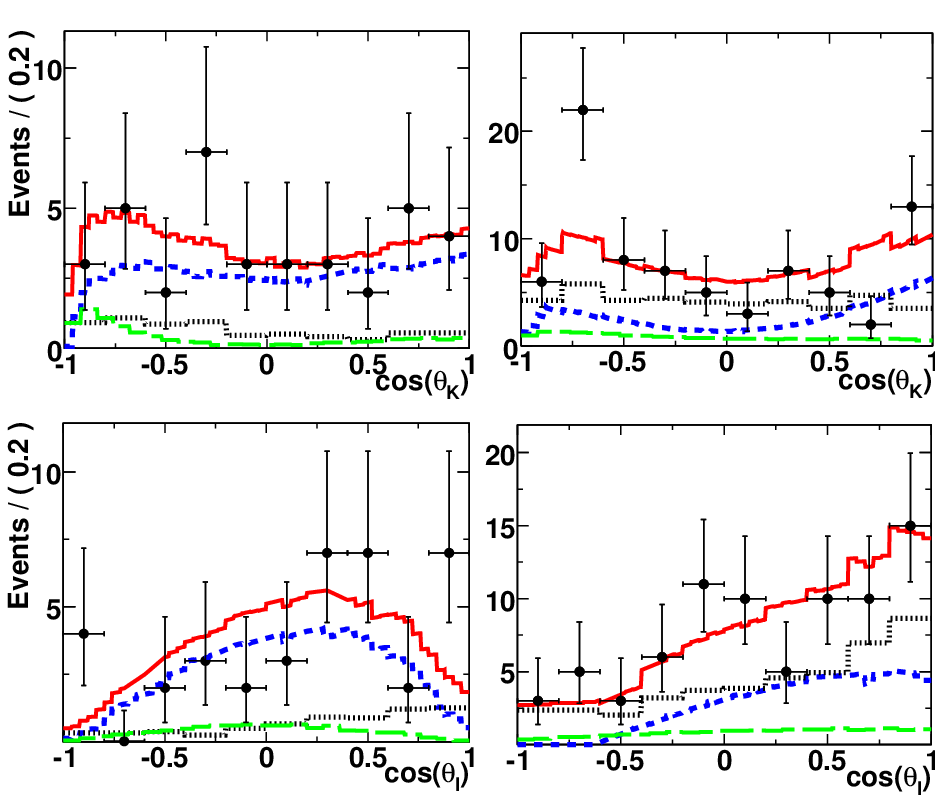
Figure 23 shows the $\cos\theta_{K}$ and $\cos\theta_{\ell}$ distributions for the six $K^{*}\ell^{+}\ell^{-}$ modes combined in the low $q^{2}$ and high $q^{2}$ regions. The fits include pdf shapes of the signal, combinatorial background, peaking backgrounds, and backgrounds from misidentified muons. In the low $q^{2}$ and high $q^{2}$ regions we measure

and

Figures 24 show these results in comparison to the SM prediction and expectations of the three other models introduced in chapter II. Though consistent with the SM prediction, the results for ${\cal F}_{L}$ and ${\cal A}_{FB}$ favor the flipped-sign $\widetilde{C}_{7}$ model [22]. Figure 25 shows our ${\cal A}_{FB}$ results in comparison to the present Belle results [38]. In the Belle analysis the low $q^{2}$ region is divided into two bins where the high bin extends to $8.7~\rm GeV^{2}/c^{4}$. The high $q^{2}$ region is divided into a bin between the $J/\psi$ and $\psi(2S)$ resonances and two bins above the $\psi(2S)$. The results of both experiments are in good agreement and the Belle results also favor the flipped-sign $\widetilde{C}_{7}$ model. The large values of ${\cal A}_{FB}$ in the high $q^{2}$-region disfavor the wrong-sign $\widetilde{C}_{9}\widetilde{C}_{10}$ model at the $>3\sigma$ level. Obviously, we need to perform a model-independent global fit to measurements of ${\cal A}_{FB}$, ${\cal F}_{L}$ and other observables using data from BABAR and Belle to look for significant discrepancies to the SM predictions and to extract non-SM contributions in the effective Wilson coefficients $\widetilde{C}_{7}$, $\widetilde{C}_{9}$ and $\widetilde{C}_{10}$. This, however, may require more precise results than are presently available. In addition, it would be useful to include measurements of other electroweak penguin decays such as $B\rightarrow X_{s}\ell^{+}\ell^{-}$ in the fit.