Gauge fields and curvature in graphene
Abstract
The low energy excitations of graphene can be described by a massless Dirac equation in two spacial dimensions. Curved graphene is proposed to be described by coupling the Dirac equation to the corresponding curved space. This covariant formalism gives rise to an effective hamiltonian with various extra terms. Some of them can be put in direct correspondence with more standard tight binding or elasticity models while others are more difficult to grasp in standard condensed matter approaches. We discuss this issue, propose models for singular and regular curvature and describe the physical consequences of the various proposals.
pacs
75.10.Jm, 75.10.Lp, 75.30.DsI Introduction
Since its experimental realization graphene has been a focus of intense research activity both theoretical and experimentally as can be seen in the recent reviews [1, 2, 3, 4]. The origin of this interest lies partially on the experimental capability to tailoring the samples into special geometries leading to graphene based electronics but it is its unusual electronic properties and the breakdown of the standard Fermi liquid description what has lead the main activity in the field. Despite the intense research three aspects of the electronic properties remain to be fully understood: that of the minimal conductivity [5, 6, 7], the observed charge inhomogeneities at low densities [8], and the exceptionally high mobility at room temperature with an associated mean free path of the order of the size of the samples [9, 10]. A key point to understand all the three problems is a better knowledge of the nature and effect of disorder in graphene.
One of the most intriguing properties of the suspended graphene samples is the observation of mesoscopic corrugations in both suspended [11, 12] and deposited on a substrate [13, 14] samples whose possible influence on the electronic properties only now starts to be realized [11, 15, 16, 17, 18, 19]. Although the observed ripples were invoked from the very beginning to explain the absence of weak localization in the samples [20, 21], there have been so far few attempts to model the corrugations. The two main approaches are based either on the presence of disclinations and other topological defects in the graphene lattice [22, 23] or on the theory of elasticity [11, 15, 16]. The concrete realization of both models in the continuum gives rise to the appearance of gauge fields coupled to the electronic degrees of freedom [24]. In this work we will describe two different approaches to model curvature in graphene and study its influence on the physical properties of the material.
II A summary of graphene features
Under a theoretical point of view the synthesis of graphene has opened a new world where ideas from different branches of physics can be confronted and tested in the laboratory. On the electronic point of view it can be shown that the low energy excitations of the neutral system obey a massless Dirac equation in two dimensions. This special behavior originates on the geometry and topology of the honeycomb lattice and has profound implications to the transport and optical properties. Although the Fermi velocity is approximately a hundredth of the speed of light, the masslessness of the quasiparticles brings the physics to the domain of relativistic quantum mechanics where phenomena like the Klein paradox or the Zitterbewegung [2] can be explored. None of these questions arise within the quantum field theory approach but its full applicability to the condensed matter system is questionable.


Monolayer graphite - graphene- consists of a planar honeycomb lattice of carbon atoms shown at the left hand side of Fig. 1. In the graphene structure the in-plane bonds are formed from 2, 2 and 2 orbitals hybridized in a configuration, while the 2 orbital, perpendicular to the layer, builds up covalent bonds, similar to the ones in the benzene molecule. The bonds give rigidity to the structure and the bonds give rise to the valence and conduction bands. A usual tight binding analysis of the system [25, 26] leads to a special band structure shown at the right hand side of Fig. 1. The Fermi surface of the neutral system consists of six Fermi points (only two are independent). A continuum model for the low energy excitations around the Fermi points (i=1,2) can be defined governed by the Hamiltonian
| (1) |
where are the Pauli matrices, , and is the distance between nearest carbon atoms. The components of the two-dimensional wavefunction:
| (2) |
correspond to the amplitude of the wave function in each of the two sublattices (A and B) which build up the honeycomb structure and the subindex refers to the two Fermi points. It can be shown that the wave function (2) transforms as a bispinor in k-space and it acquires a phase of under a rotation. This Berry phase together with the helicity conservation has important physical consequences as the absence of backward scattering in the electronic transport what implies the absence of weak localization.
The spinor structures around each of the two Fermi points remain degenerate and independent in the absence of short range interactions of disorder. As we will see, topological disorder mixes the two Fermi points and in the modelling of them it will be useful to combine the two bispinors into a four dimensional object described by the effective Hamiltonian
| (3) |
where and matrices are Pauli matrices acting on the sublattice and valley degree of freedom respectively.
III Modelling curvature in graphene
When trying to take into account the curvature of the graphene samples and its physical implications there are two aspects to consider: The first and of the most interesting questions is the physical origin of the ripples and their dynamics. The present experimental situation seems to indicate that there is little dependence of the corrugations with temperature –although systematic studies have not been performed yet –. On the other hand, bilayer structures also present corrugations but less pronounced [15]. These aspects concern the sigma bonds of graphene and their elastic properties and involve energies of the order of tens of eV. Although the elastic and mechanical properties of carbon nanotubes have been extensively explored [27], very little can yet be found on the elastic properties of plain graphene [28].
A second aspect is that of the influence of the ripples on the electronic properties of the samples. A possible approach to this problem is to assume that the samples are corrugated for whatever reason and devise a model to study the implications of the corrugations on the electronic properties. This is a sensible procedure considering that the electronic properties of graphene are attached to the bonds and the associated processes involve energies several orders of magnitude smaller than those related to the elasticity of the bonds.
Since the low energy excitations of graphene are well described by the massless Dirac equation, a natural way to incorporate the effect of the observed corrugations at low energies is couple the Dirac equation to the given curved background. The main assumption of this approach is that the elastic properties of the samples –determined by the sigma bonds – are decoupled from the (pi) electron dynamics. The ripples can then be modelled by a fixed metric space defined phenomenologically from the observed corrugations and the electronic properties of the system will be found from the computation the Green’s function in the curved space following the standard formalism set in gravitational physics [29, 30].
Although the physical origin of the ripples is unknown, we could distinguish two possibilities: those coming from the curvature in the substrate [14] that can be modelled by a smooth curved space and those observed in the free standing samples. The last class needs to be modelled by including topological defects [31]: disclinations and disclination dipoles (dislocations). In what follows we will summarize the general formalism to include a curved background and to extract the physical implications.
The dynamics of a massless Dirac spinor in a curved spacetime is governed by the modified Dirac equation:
| (4) |
The curved space matrices depend on the point of the space and can be computed from the anticommutation relations
The covariant derivative operator is defined as
where is the spin connection of the spinor field that can be calculated using the tetrad formalism[29].
Once the metric of the curved space is known there is a standard procedure to get the geometric factors that enter into the Dirac equation. In the modelling of the graphene ripples, the metric can be treated as a smooth perturbation of the flat surface and physical results are obtained by a kind of perturbation theory. Very often, the final result can be cast in the form of the flat Dirac problem in the presence of an effective potential induced by the curvature.
The electronic properties of the curved sample can be extracted from the two point Green’s function. The equation for the exact propagator in the curved space-time is:
| (5) |
where is the spin connection and is the determinant of the metric. From the propagator one can compute the local density of states:
| (6) |
and other one-particle properties of the system as the electron lifetime.
The described formalism can in principle be worked out for any curved background. The practical difficulties to implement this scheme are related with the choice of a realistic metric parametrizing the graphene sheet and to the ability to perform a ”weak field” expansion of the metric around the flat case. In the next sections we will see the mechanism at work in two quite general examples.
IV Smooth ripples from the substrate
The case of smooth curvature was studied in reference [17] where a general metric was considered that was non-singular over the surface and asymptotically flat. The embedding of a two-dimensional surface with polar symmetry –for simplicity– in three-dimensional space is described in cylindrical coordinates by a function giving the height with respect to the flat surface z=0, and parametrized by the polar coordinates of its projection onto the z=0 plane. The metric for this surface is readily obtained by computing
| (7) |
and substituting for the line element:
| (8) |
where is a smooth function with the appropriate asymptotic behavior and the parameter controls the deviations from flat space. The advantage of this approach is that it provides already the perturbative parameter needed to compute the electron propagator.
A concrete example is provided by the gaussian shape shown at the left hand side of fig. 2. It models a smooth protuberance fitting without singularities in the average flat graphene sheet.
| (9) |
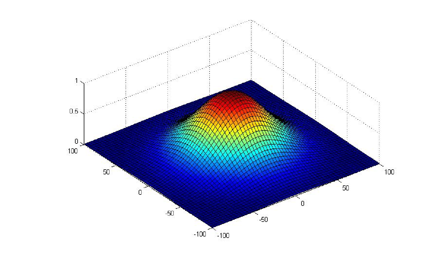
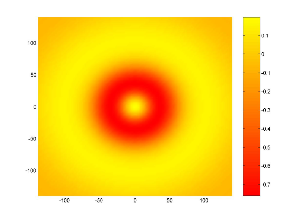
This example was worked out in full detail in ref. [17]. A comparison of the Dirac Hamiltonian in the plane (flat) in polar coordinates
| (10) |
with the corresponding curved hamiltonian
| (11) |
| (12) |
allows to extract the two main features of the model. First we can see that the curved bump produces an effective Fermi velocity in the radial direction given by
| (13) |
The effective Fermi velocity will always be smaller in magnitude than the flat one. For a general curved surface described in polar coordinates by an arbitrary function it will be
| (14) |
In a more general case we will have the two components of the velocity changed but always to a smaller value irrespective of the sign of the curvature at the given point.
The second feature that arises is an effective magnetic field perpendicular to the graphene sheet given by
| (15) |
The electronic properties of the curved sample were computed from the electron propagator to first order in the small parameter that measures the deviation from flat space. In our example, is the (squared) height to length ratio of the gaussian, so for typical ripples in graphene , since this ratio is of the order of 0.1 [11]. They are shown in the right hand side of Fig. 2. As a general feature the curvature induces inhomogeneities in the electronic density of states that could be related to the observations reported in [8]. It is worth noticing that the contribution of the effective gauge field coming from the spin connection to first order in perturbation theory vanishes and all the corrections come from the determinant of the metric and the curved gamma matrices. This is important when trying to compare the present formalism with the tight binding modelling of curvature where only the gauge field arises from the modulation of the hopping parameter.
V Topological defects
In the absence of a substrate or strain fields the only way to have intrinsic curvature in the samples is by the presence of topological defects [31]. In the case of the hexagonal lattice of graphene disclinations form by replacing a hexagon of the lattice by a n–sided polygon with . The most common disclination in graphene is the pentagon that plays an important role in the formation of fullerenes [32]. Dislocations are made of pentagon–heptagon pairs and they have been widely studied in connection with the properties of carbon nanotubes [27] and, more recently, in graphene [33, 34, 35, 36]. Observation of topological defects in graphene have been reported in [37, 38, 39].
Following the discovery of the fullerenes and nanotubes topological defects have been modelled in the hexagonal lattice in different ways. A very interesting approach related with the theory of elasticity is the gauge theory of the defects described in refs. [40, 41, 42, 43] or the metric formulation of the theory of defects in solids set in [44]. Most of these approaches model the topological defects focussing on their ”holonomy” [45, 46, 47, 48, 49]and very little effort has been devoted to the specific issue of the curvature in these cases. The curvature of the graphene surface in the presence of a disclination in the continuum limit has a delta-function singularity at the position of the defective ring. In modelling spherical [45, 46] and quasi-spherical [50, 51] fullerenes curvature effects are included but the curvature is averaged along the spherical surface. The more difficult task of modelling several topological defects located at arbitrary positions was undertaken in refs. [22, 23]. An equal number of pentagon and heptagon defects was considered to keep the samples flat in average. The proposed metric was taken from the cosmic string scenario:
| (16) |
where
and
This metric describes the space-time around N parallel cosmic strings, located at the points . The parameters are related to the angle defect or surplus by the relation in such manner that if then . Within the formalism described earlier it can be seen that the Green’s function is modified by the potential
| (17) |
The computation of the corrections to the local density of states for different positions of the defects showed that pentagonal (heptagonal) rings enhance (depress) the electron density, a result that was obtained previously [52] with numerical simulations. Numerical ab initio calculations show sharp resonant peaks in the LDOS at the tip apex of nanocones [52, 53] that have been proposed for electronic applications in field emission devices. Similar results have also been obtained analytically in [54]. A recent calculation of the minimal conductivity in graphene with a random distribution of heptagon and pentagon rings bases on this model has been performed in [55].
VI Conclusions and future
From the present and similar analyses we can conclude that the morphology of the graphene samples is correlated with the electronic properties. In particular the presence of ripples, irrespective of their origin, induces corrections to the density of states and affects the transport properties. The spatial variation of the Fermi velocity is a distinctive prediction of the given geometric formalism. We note that the effective Fermi velocity is the fitting parameter used in most experiments [8] whose interpretation might change if the possibility of a space-dependent velocity is considered.
Gauge fields are abundant in graphene and arise in many different contexts. This is partially a proof of the robustness of the Dirac formulation where only minimal coupling in the form of electronic current-vector field are marginal interactions to be considered at low energies [56]. They arise in various contexts and it would be interesting to have a complete classification. In the present context it is interesting to note the work of [57] where it was shown that, around each Fermi point, static strains can mimic the effects of external electric and magnetic fields.
Future work should address a better understanding of the mechanisms leading to ripple formation and elastic properties of graphene. There is also little work done on transport and localization properties of graphene in the presence of topological defects, a very important issue.
Acknowledgments
This work is support by MEC (Spain) through grant FIS2005-05478-C02-01 and by the European Union Contract 12881 (NEST) Ferrocarbon.
References
- [1] A. K. Geim and K. S. Novoselov, Nature 6, 183 (2007).
- [2] M. I. Katsnelson and K. Novoselov, Solid State Communications 143, 3 (2007).
- [3] V. Gusynin, S. Sharapov, and J. Carbotte, International Journal of Modern Physics B 21, 4611 (2007).
- [4] A. H. C. Neto, F. Guinea, N. M. R. Peres, K. S. Novoselov, and A. K. Geim, Reviews of Modern Physics (2008).
- [5] K. S. Novoselov, A. K. Geim, S. V. Morozov, D. Jiang, M. I. Katsnelson, I. V. Grigorieva, S. V. Dubonos, and A. A. Firsov, Nature 438, 197 (2005).
- [6] Y. Zhang, Y.-W. Tan, H. L. Stormer, and P. Kim, Nature 438, 201 (2005).
- [7] J. H. Chen, C. Jang, M. S. Fuhrer, E. D. Williams, and M. Ishigami (2008), eprint arxiv0708.2408.
- [8] J. Martin, N. Akerman, G. Ulbricht, T. Lohmann, J. H. Smet, K. von Klitzing, and A. Yacoby, Nature Physics 4, 144 (2008).
- [9] K. I. Bolotin, K. J. Sikes, Z. Jiang, G. Fudenberg, J. Hone, P. Kim, and H. L. Stormer (2008), eprint arXiv:0802.2389.
- [10] X. Du, I. Skachko, A. Barker, and E. Y. Andrei (2008), eprint arXiv:0802.2933.
- [11] J. C. Meyer, A. K. Geim, M. I. Katsnelson, K. S. Novoselov, T. J. Booth, and S. Roth, Nature 446, 60 (2007a).
- [12] T. J. Booth, P. Blake, R. R. Nair, D. Jiang, E. W. Hill, U. Bangert, A. Bleloch, M. Gass, K. S. Novoselov, M. I. Katsnelson, et al. (2008), eprint 0805.1884.
- [13] E. Stolyarova, K. T. Rim, S. Ryu, J. Maultzsch, P. Kim, L. E. Brus, T. F. Heinz, M. S. Hybertsen, and G. W. Flynn, PNAS 104, 9209 (2007).
- [14] M. Ishigami, J. H. Chen, W. G. Cullen, M. S. Fuhrer, and E. D. Williams, Nano Letters 7, 1643 (2007).
- [15] J. C. Meyer, A. K. Geim, M. I. Katsnelson, K. S. Novoselov, D. Obergfell, S. Roth, C. Girit, and A. Zettl, Solid State Communication 143, 101 (2007b).
- [16] A. Castro-Neto and E. Kim (2007), eprint cond-mat/0702562.
- [17] F. de Juan, A. Cortijo, and M. A. H. Vozmediano, Phys. Rev. B 76, 165409 (2007).
- [18] F. Guinea, M. Katsnelson, and M. A. H. Vozmediano, Phys. Rev. B 77, 075422 (2008a).
- [19] L. Brey and J. J. Palacios, Phys. Rev. B 77, 041403(R) (2008).
- [20] S. V. Morozov, K. S. Novoselov, M. I. Katsnelson, F. Schedin, L. A. Ponomarenko, D. Jiang, and A. K. Geim, Phys. Rev. Lett. 97, 016801 (2006).
- [21] A. F. Morpurgo and F. Guinea, Phys. Rev. Lett. 97, 196804 (2006).
- [22] A. Cortijo and M. A. H. Vozmediano, Eur. Phys. Lett. 77, 47002 (2007a).
- [23] A. Cortijo and M. A. H. Vozmediano, Nucl. Phys. B 763, 293 (2007b).
- [24] F. Guinea, B. Horovitz, and P. L. Doussal, Phys. Rev. B 77, 205421 (2008b).
- [25] P. R. Wallace, Phys. Rev. 71, 622 (1947).
- [26] J. C. Slonczewski and P. R. Weiss, Phys. Rev. 109, 272 (1958).
- [27] R. Saito, G. Dresselhaus, and M. S. Dresselhaus, Physical Properties of Carbon Nanotubes (World Scientific, 1998).
- [28] J. Atalaya, A. Isacsson, and J. M. Kinaret (2008), eprint arXiv:0806.2576.
- [29] N. D. Birrell and P. C. W. Davis, Quantum fields in curved space (Cambridge University Press, 1982).
- [30] S. Weinberg, The quantum theory of fields (Cambridge University Press, 1996).
- [31] D. R. Nelson, Defects and geometry in condensed matter physics (Cambridge University Pres, 2002).
- [32] H. W. Kroto, J. R. Heath, S. C. OBrien, R. F. Curl, and R. E. Smalley, Nature 318, 162 (1985).
- [33] A. Anokhin, M. N. Gal’perin, Y. N. Gornostyrev, and M. I. Katsnelson, JETP Lett. 59, 369 (1994).
- [34] A. Carpio and L. L. Bonilla (2008), eprint arXiv:0805.1220.
- [35] A. Carpio, L. L. Bonilla, F. de Juan, and M. A. H. Vozmediano, New J. Phys. 10, 053021 (2008).
- [36] M. P. López-Sancho, F. de Juan, and M. A. H. Vozmediano (2008), eprint arXiv:0806.3000.
- [37] B. An, S. Fukuyama, K. Yokogawaa, M. Yoshimura, M. Egashira, Y. Korai, and I. Mochida, Appl. Phys. Lett. 23 (2001).
- [38] A. Hashimoto, K. Suenaga, A. Gloter, K. Urita, and S. Iijima, Nature 430, 870 (2004).
- [39] E. J. Duplock, M. Scheffler, and P. J. D. Lindan, Phys. Rev. Lett. 92 (2004).
- [40] H. Kleinert, Gauge fields in condensed matter, vol. 2 (World Scientific, Singapore, 1989).
- [41] E. A. Kochetov and V. A. Osipov, J. Phys. A 32, 1961 (1999).
- [42] V. A. Osipov, E. A. Kochetov, and M. Pudlak, JETP 73, 562 (2003).
- [43] C. Furtado, A. M. de M. Carvalho, and C. A. de Lima Ribeiro, Mod. Phys. Lett. A 21, 1393 (2006a).
- [44] M. O. Katanaev and I. V. Volovich, Annals of Physics 216, 1 (1992).
- [45] J. González, F. Guinea, and M. A. H. Vozmediano, Phys. Rev. Lett. 69, 172 (1992).
- [46] J. González, F. Guinea, and M. A. H. Vozmediano, Nucl. Phys. B 406 [FS], 771 (1993).
- [47] P. E. Lammert and V. H. Crespi, Phys. Rev. Lett. 85, 5190 (2000).
- [48] V. A. Osipov and E. A. Kochetov, JETP Lett. 73, 562 (2001).
- [49] C. Furtado, F. Moraes, and A. M. de M. Carvalho (2006b), eprint cond-mat/0601391.
- [50] D. Kolesnikov and V. A. Osipov, European Physical Journal B 49, 465 (2006).
- [51] M. Pudlak, R. Pincak, and V. A. Osipov, Phys. Rev. B 74, 235435 (2006).
- [52] R. Tamura and M. Tsukada, Phys. Rev. B. 49, 7697 (1994).
- [53] J. C. Charlier and G. M. Rignanese, Phys. Rev. Lett. 86, 5970 (2001).
- [54] Y. Sitenko and N. Vlasii, Nucl. Phys. B 787, 241 (2007).
- [55] A. Cortijo and M. A. H. Vozmediano (2007c), eprint arXiv:0709.2698.
- [56] J. González, F. Guinea, and M. A. H. Vozmediano, Nucl. Phys. B 424 [FS], 595 (1994).
- [57] J. L. Mañes, Phys. Rev. B 76, 045430 (2007).