Measurement of beam-recoil observables $O_{x}$ , $O_{z}$ and target asymmetry for the reaction $\gamma p\rightarrow K^{+}\Lambda$

For the present results, the charged decay of the $\Lambda$ ($\Lambda\rightarrow p\pi^{-}$, BR=63.9%) was considered and the same selection method used in our previous publication on $K\Lambda$ photoproduction [5] was applied. Only the main points will be recalled in the following.

Only events with three tracks and no neutral cluster detected in the BGO calorimeter were retained. In the absence of a direct measurement of energy and/or momentum of the charged particles, the measured angles ($\theta$, $\varphi$) of the three tracks were combined with kinematical constraints to calculate momenta. Particle identification was then obtained from the association of the calculated momenta with dE/dx and/or ToF measurements.

The main source of background is the $\gamma p\rightarrow p\pi^{+}\pi^{-}$ reaction, a channel with a similar final state and a cross section hundred times larger. Selection of the $K\Lambda$ final state was achieved by applying narrow cuts on the following set of experimental quantities:

• .

  Energy balance.

• .

  Effective masses of the three particles extracted from the combination of measured dE/dx and ToF (only at forward angles) with calculated momenta.

• .

  Missing mass $m_{\gamma p-K^{+}}$ evaluated from $E_{\gamma}$, $\theta_{K}$ (measured) and $p_{K}$ (calculated).

For each of these variables, the width $\sigma$ of the corresponding distribution (Gaussian-like shape) were extracted from a Monte-Carlo simulation of the apparatus response based on the GEANT3 package of the CERN library.

To check the quality of the event selection, the distribution of the $\Lambda$ decay length was used due to its high sensitivity to background contamination.

Event by event, track information and $\Lambda$ momentum were combined to obtain the distance $d$ between the reaction and decay vertices. The $\Lambda$ decay length was then calculated with the usual formula $ct_{\Lambda}=d/(\beta_{\Lambda}*\gamma_{\Lambda})$. Fig. 2 shows the resulting distributions for events selected with all cuts at $\pm$2$\sigma$ (closed circles) compared with events without cuts (open circles). These spectra were corrected for detection efficiency losses estimated from the Monte-Carlo simulation (significant only for ct$\geq$5 cm). It should be noted that the deficit in the first bins is attributed to finite resolution effects not fully taken into account in the simulation.

The first spectrum was fitted for ct$\geq$1 cm by an exponential function $\alpha*exp(-ct/c\tau)$ with $\alpha$ and $c\tau$ as free parameters. The fitted $c\tau$ value (8.17$\pm$0.31 cm) is in good agreement with the PDG expectation for the $\Lambda$ mean free path ($c\tau_{\Lambda}$=7.89 cm) [9].

By contrast, the spectrum without cuts is dominated by $p\pi^{+}\pi^{-}$ background events. As expected, they contribute mostly to small ct values ($\leq$2-3 cm), making the shape of this distribution highly sensitive to background contamination. For instance, a pronounced peak already shows up when opening selection cuts at $\pm$3$\sigma$.

A remaining source of background, which cannot be seen in the ct plot presented above, originates from the contamination by the reaction $\gamma p\rightarrow K^{+}\Sigma^{0}$. Indeed, events where the decay photon is not detected are retained by the first selection step. Since these events are kinematically analyzed as $K\Lambda$ ones, most of them are nevertheless rejected by the selection cuts. From the simulation, this contamination was found to be of the order of 2%.

As a further check of the quality of the data sample, the missing mass spectrum was calculated. One should remember that the missing mass is not directly measured and is not used as a criterion for the channel identification. The spectrum presented in fig. 3 (closed circles) is in fair agreement with the simulated distribution (solid line). Some slight discrepancies can nevertheless be seen in the high energy tail of the spectra. The simulated missing mass distribution of the contamination from the $\gamma p\rightarrow K^{+}\Sigma^{0}$ reaction, also displayed in fig. 3, clearly indicates that such a background cannot account for the observed differences. Rather, these are attributed to the summation of a large number of data taking periods with various experimental configurations (target length, wire chambers, green vs UV laser line, …). Although these configurations were implemented in corresponding simulations, small imperfections (misalignments in particular) could not be taken into account.

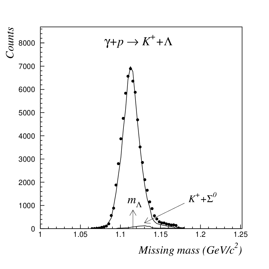
To summarize, thanks to these experimental checks, we are confident that the level of background in our selected sample is limited. This is corroborated by the simulation from which the estimated background contamination (multi-pions and $K^{+}\Sigma^{0}$ contributions) never exceeds 5% whatever the incident photon energy or the meson recoil angle.

As will be shown below, the beam-recoil observables $O_{x}$ and $O_{z}$, as well as the target asymmetry $T$, can be extracted from the angular distribution of the $\Lambda$ decay proton.

In pseudoscalar meson photoproduction, one can extract experimentally 16 different quantities: the unpolarized differential cross section $(d\sigma/d\Omega)_{0}$, 3 single polarization observables ($P$, $T$, $\Sigma$), 4 beam-target polarizations ($E$, $F$, $G$, $H$), 4 beam-recoil polarizations ($C_{x}$, $C_{z}$, $O_{x}$, $O_{z}$) and 4 target-recoil polarizations ($T_{x}$, $T_{z}$, $L_{x}$, $L_{z}$). The various spin observables are not independent but are constrained by non-linear identities and various inequalites [10], [11], [14], [15]. In particular, of the seven single and beam-recoil polarization observables, only five are independent being related by the two equations:

These different identities and inequalities can be used to test the consistency of our present and previous measurements. They can also be used to check the compatibility of our data with the results on $C_{x}$ and $C_{z}$ recently published by the CLAS collaboration [7].

Our measured values for $\Sigma$, $P$, $T$, $O_{x}$ and $O_{z}$ were combined to test the above inequalities. Equation 31 was used to calculate the quantity $C_{x}^{2}+C_{z}^{2}$ appearing in expressions 36 and 37. The results for the two combinations $|T\pm P|\mp\Sigma$ of the three single polarizations are presented in fig. 12. The results for the quantities:

• .

  $(P^{2}+O_{x}^{2}+O_{z}^{2})^{1/2}$,

• .

  $(\Sigma^{2}+O_{x}^{2}+O_{z}^{2})^{1/2}$,

• .

  $(1+T^{2}-P^{2}-O_{x}^{2}-O_{z}^{2})^{1/2}=(\Sigma^{2}+C_{x}^{2}+C_{z}^{2})^{1/2}$,

• .

  $(1+T^{2}-\Sigma^{2}-O_{x}^{2}-O_{z}^{2})^{1/2}=(P^{2}+C_{x}^{2}+C_{z}^{2})^{1/2}$,

Since all observables entering in eqs. 31 and 32 were measured either by GRAAL ($\Sigma$, $P$, $T$, $O_{x}$, $O_{z}$) or by CLAS ($P$, $C_{x}$, $C_{z}$ - their $P$ data were confirmed by our measurements [5]), the two sets of data can be therefore compared and combined. Within the error bars, the agreement between the two sets of equal combinations $(1+T^{2}-\Sigma^{2}-O_{x}^{2}-O_{z}^{2})^{1/2}$ (GRAAL) and $(P^{2}+C_{x}^{2}+C_{z}^{2})^{1/2}$ (CLAS) is fair (fig. 14) and tends to confirm the previously observed saturation to the value 1 of $R=(P^{2}+C_{x}^{2}+C_{z}^{2})^{1/2}$, whatever the energy or angle. Fig. 15 displays the values for the combined GRAAL-CLAS quantity $C_{z}O_{x}-C_{x}O_{z}-T+P\Sigma$. Within the uncertainties, the expected value (1) is obtained, confirming again the overall consistency of the GRAAL and CLAS data.

It has been demonstrated [14] that the knowledge of the unpolarized cross section, the three single-spin observables and at least four double-spin observables - provided they have not all the same type - is sufficient to determine uniquely the four complex reaction amplitudes. Therefore, only one additional double polarization observable measured using a polarized target will suffice to extract unambiguously these amplitudes.

We have compared our results with two models: the Ghent isobar RPR (Regge-plus-resonance) model [16]-[19] and the coupled-channel partial wave analysis developed by the Bonn-Gatchina collaboration [20]-[24]. In the following, these models will be refered as RPR and BG, respectively. The comparison is shown in figs. 9 to 11.

The RPR model is an isobar model for $K\Lambda$ photo- and electroproduction. In addition to the Born and kaonic contributions, it includes a Reggeized t-channel background which is fixed to high-energy data. The fitted database includes differential cross section, beam asymmetry and recoil polarization photoproduction results. The model variant presented here contains, besides the known $N^{*}$ resonances ($S_{11}$(1650), $P_{11}$(1710), $P_{13}$(1720)), the $P_{13}$(1900) state (** in the PDG [9]) and a missing $D_{13}$(1900) resonance. This solution was found to provide the best overall agreement with the combined photo- and electroproduction database. As one can see in figs. 9 to 11, the RPR prediction (dashed line) qualitatively reproduces all observed structures. Interestingly enough, the model best reproduces the data at high energy (1400-1500 MeV), where the $P_{13}$(1900) and $D_{13}$(1900) contributions are maximal.

The BG model is a combined analysis of experiments with $\pi N$, $\eta N$, $K\Lambda$ and $K\Sigma$ final states. As compared to the other models, this partial-wave analysis takes into account a much larger database which includes most of the available results (differential cross sections and polarization observables). For the $\gamma p\rightarrow K^{+}\Lambda$ reaction, the main resonant contributions come from the $S_{11}$(1535), $S_{11}$(1650), $P_{13}$(1720), $P_{13}$(1900) and $P_{11}$(1840) resonances. To achieve a good description of the recent $C_{x}$ and $C_{z}$ CLAS measurements, the ** $P_{13}$(1900) had to be introduced. It should be noted that, at this stage of the analysis, the contribution of the missing $D_{13}$(1900) is significantly reduced as compared to previous versions of the model. As shown in figs. 9-11, this last version (solid line) provides a good overall agreement. On the contrary, the solution without the $P_{13}$(1900) (not shown) fails to reproduce the data.

More refined analyses with the RPR and BG models are in progress and will be published later on. Comparison with the dynamical coupled-channel model of Saclay-Argonne-Pittsburgh [25]-[27] has also started.

References

- (1) R.K.Bradford et al., Phys. Rev. C 73, 035202 (2006).
- (2) K.-H. Glander et al., Eur. Phys. J. A 19, 251 (2004).
- (3) J.W.C. McNabb et al., Phys. Rev. C 69, 042201(R) (2004).
- (4) M. Sumihama et al., Phys. Rev. C 73, 035214 (2006).
- (5) A. Lleres et al., Eur. Phys. J. A 31, 79 (2007).
- (6) R.G.T. Zegers et al., Phys. Rev. Lett. 91, 092001 (2003).
- (7) R.K.Bradford et al., Phys. Rev. C 75, 035205 (2007).
- (8) O. Bartalini et al., Eur. Phys. J. A 26, 399 (2005).
- (9) Review of Particle Physics 2004, Phys. Lett. B 592, 1 (2004).
- (10) R.A. Adelseck and B. Saghai, Phys. Rev. C 42, 108 (1990).
- (11) I.S. Barker, A. Donnachie and J.K. Storrow, Nucl. Phys. B 95, 347 (1975).
- (12) P. Calvat, Thesis, Université J. Fourier Grenoble, 1997, unpublished.
- (13) T.D. Lee and C.N. Yang, Phys. Rev. 108, 1645 (1957).
- (14) W.T. Chiang and F. Tabakin, Phys. Rev. C 55, 2054 (1997).
- (15) X. Artru, J.M. Richard and J. Soffer, Phys. Rev. C 75, 024002 (2007).
- (16) T. Corthals, J. Ryckebusch and T. Van Cauteren, Phys. Rev. C 73, 045207 (2006).
- (17) T. Corthals, Thesis, Universiteit Gent, 2007, unpublished.
- (18) T. Corthals et al., Phys. Lett. B 656, 186 (2007).
- (19) T. Corthals, J. Ryckebusch and P. Vancraeyveld, private communication.
- (20) A.V. Anisovich et al., Eur. Phys. J. A. 25, 427 (2005).
- (21) A.V. Sarantsev et al., Eur. Phys. J. A. 25, 441 (2005).
- (22) A.V. Anisovich et al., Eur. Phys. J A 34, 243 (2007).
- (23) V.A. Nikonov et al., arXiv:hep-ph/0707.3600 (2007).
- (24) A. Sarantsev, private communication.
- (25) B. Juliá-Díaz, B. Saghai, T.-S.H. Lee and F. Tabakin, Phys. Rev. C 73, 055204 (2006).
- (26) B. Saghai, J.C. David, B. Juliá-Díaz and T.-S.H. Lee, Eur. Phys. J. A 31, 512 (2007).
- (27) B. Saghai, private communication.