Exclusive $\rho^{0}$ electroproduction on the proton at CLAS

The electron is identified as a negative track, determined from the DC, having produced a signal in the CC and the EC. Pions, potentially misidentified as electrons, were rejected by cutting on the CC amplitude ($>$ 2 photoelectrons), imposing a minimum energy deposition in the EC (60 MeV) and correlating the measurements of the momentum from the DC and of the energy from the EC. In order to minimize radiative corrections and residual pion contamination, a further cut E${}^{\prime}\geq$ 0.8 GeV was also applied, where E^′ is the scattered electron energy. Finally, vertex and geometric fiducial cuts, which select only regions of well understood acceptance, were included.

The efficiencies of the CC and EC cuts, respectively $\eta_{CC}$ and $\eta_{EC}$, were determined from data samples, selecting unambiguous electrons with very tight CC or EC cuts. The CC-cut efficiencies range from 86 to 99% and the EC-cut efficiencies from 90 to 95%, depending on the electron kinematics. The efficiencies of the geometric fiducial cuts were derived from CLAS GEANT-based Monte-Carlo simulations.

Pions and protons are identified by the correlation between the momentum measured by the DC and the velocity measured by the SC. This identification procedure is unambiguous for particles with momenta up to 2 GeV. Particles with momenta higher than 2 GeV were therefore discarded. The efficiencies of the cuts imposed for this momentum-velocity correlation and of the geometric fiducial cuts were determined from CLAS GEANT-based Monte-Carlo simulations.

Once the electron, the proton and the positive pion are identified, the $ep\rightarrow e^{\prime}p\pi^{+}\pi^{-}$ final state is identified through the missing mass technique. Fig. 2 shows the square of the missing mass for the system $e^{\prime}p\pi^{+}$ (i.e. $M_{X}^{2}[e^{\prime}p\pi^{+}X]$) as a function of the missing mass for the system $ep$ (i.e. $M_{X}[e^{\prime}pX]$). One distinguishes the $\rho^{0}$ and $\omega$ loci quite clearly. A cut on the $M_{X}^{2}[e^{\prime}p\pi^{+}X]$ variable is required in order to separate the $\rho^{0}$ and the associated $\pi^{+}\pi^{-}$ continuum from the $\omega$ and the three–pion continuum background. The optimum value of this cut:

was determined from a study whereby we estimated the number of $\rho^{0}$ events, from fits to the $M_{X}^{2}[e^{\prime}pX]$ distribution, as a function of the cut values. The cuts were chosen in the region where the number of $\rho^{0}$ events began to vary only very weakly with these cut values.The simulation used to calculate acceptances reproduces the features of fig. 3. The position of this cut relative to $M_{X}^{2}[e^{\prime}p\pi^{+}X]$ is shown in fig. 3.

The missing mass distribution for the system $ep$, obtained after this cut, is shown in fig. 4. The $\rho^{0}$ peak is very broad : $\Gamma_{\rho^{0}}^{th}\approx$ 150 MeV from ref. [23]. and sits on top of a background of a non-resonant two pion continuum, which originates from other processes leading to the $e^{\prime}p\pi^{+}\pi^{-}$ final state, such as $ep\rightarrow e^{\prime}\Delta^{++}\pi^{-}\rightarrow e^{\prime}p\pi^{+}\pi^{-}$. In fig. 4, one can additionnally distinguish two bumps at masses around 950 MeV and 1250 MeV corresponding respectively to the scalar $f_{0}(980)$ and tensor $f_{2}(1270)$ mesons. These will be even more evident when we look at the differential spectra later on.

The acceptance of the CLAS detector for the $e^{\prime}p\pi^{+}X$ process has been determined with the standard GEANT-based code developed for CLAS. Our event generator [24] contains the three main channels leading to the $e^{\prime}p\pi^{+}\pi^{-}$ final state: $ep\rightarrow e^{\prime}p\rho^{0}\hookrightarrow\pi^{+}\pi^{-}$, $ep\rightarrow e^{\prime}\pi^{-}\Delta^{++}\hookrightarrow p\pi^{+}$, and the non-resonant (phase space) $ep\rightarrow e^{\prime}p\pi^{+}\pi^{-}$. This event generator is based on tables of total and differential cross sections of double pion photoproduction data that have been extrapolated to electroproduction. This has been done by multiplying these tables by a virtual photon flux factor and a dipole form factor in order to obtain a relatively realistic $Q^{2}$ dependence of the cross section. We also have tuned the relative weight of all the aforementioned channels in order to reproduce the main kinematical distributions of our experimental data.

Eight independent kinematical variables are necessary to describe a reaction with four particles in the final state. However, in unpolarized electroproduction, the cross section does not depend on the azimuthal angle of the scattered electron. The following seven variables are then chosen: $Q^{2}$, $x_{B}$, $t$, $M_{\pi^{+}\pi^{-}}$, $\Phi$, $\cos(\theta_{HS})$ and $\phi_{HS}$. Here $Q^{2}$ and $x_{B}$ are respectively the absolute value of the squared electron four-momentum transfer and the Bjorken variable, which describe the kinematics of the virtual photon $\gamma^{*}$. At some stages, $W$, the $\gamma^{*}-p$ center-of-mass energy will equivalently be used. Then $t$ is the squared four-momentum transferred to the $\rho^{0}$, $\Phi$ is the azimuthal angle between the electron scattering plane and the hadronic production plane, and $M_{\pi^{+}\pi^{-}}$ is the invariant mass of the $\pi^{+}\pi^{-}$ system. Finally, $\cos(\theta_{HS})$ and $\phi_{HS}$ describe the decay of the $\rho^{0}$ into two pions and are respectively the polar and azimuthal angles of the $\pi^{+}$ in the so-called Helicity Frame (HS) where the $\rho^{0}$ is at rest and the $z$-axis is given by the $\rho^{0}$ direction in the $\gamma^{*}-p$ center-of-mass system. All these variables are illustrated in fig. 5.

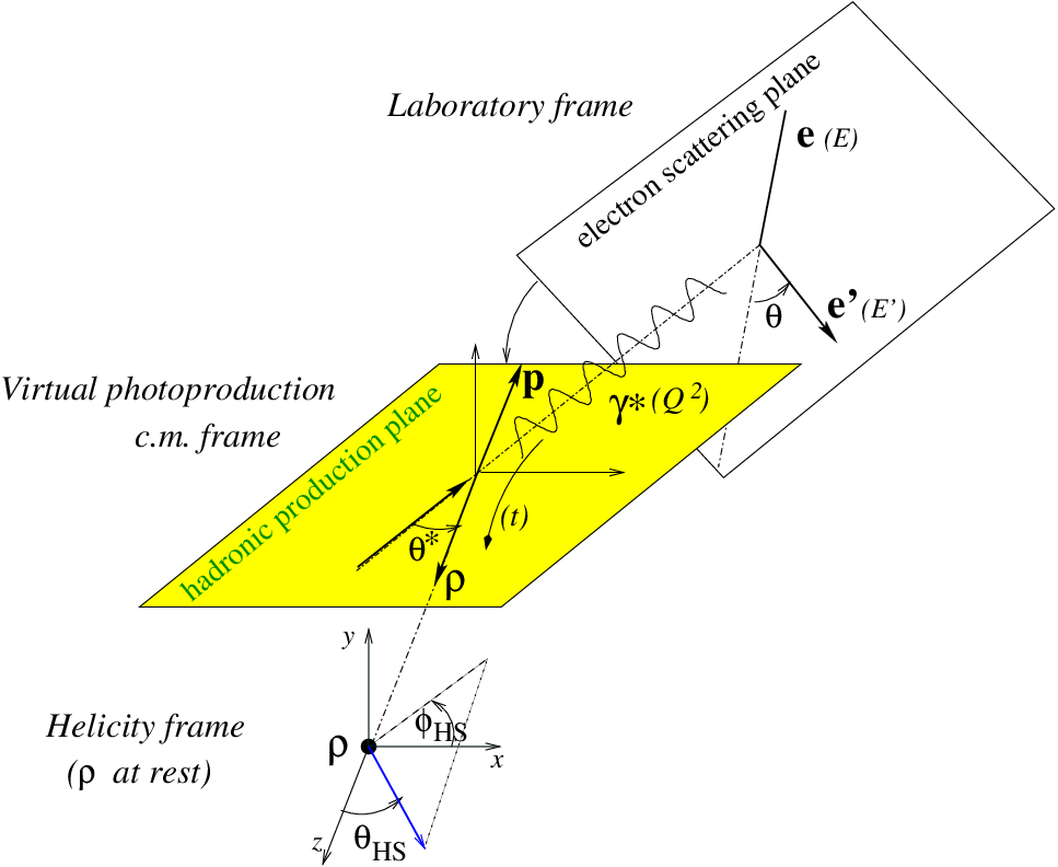
The procedure we have followed has been to calculate an acceptance for each of the 7-dimensional bins. In the limit of small bin-size and unlimited statistics, this procedure is independent of the model used to generate events. Our event generator has nonetheless been tuned to reproduce the experimental data. The binning in the 7 independent variables is defined in table 1 and its 2-dimensional ($Q^{2}$, $x_{B}$) projection is shown in fig. 6.

More than 200 million Monte-Carlo (MC) events were generated using CLAS GEANT to calculate the acceptance in each of the individual 7-dimensional bins. Each “real data” event was then weighted by the ratio of the number of MC generated to accepted events for each 7-dimensional bin. The acceptances are at most a few percent. Bins that have a very small acceptance ($<$ 0.16%) have a very high weight, which produces an unphysically high and narrow peak in the weighted event distributions, and have to be cut away. The efficiency of this cut is evaluated by MC computation of the ratio of weighted accepted events to generated events mapped onto 1-dimensional distributions. This correction factor $\eta_{w}$ is therefore model dependent since it is 1-dimensional and thus integrated over the remaining variables. It is on average 15%.

Radiative corrections were part of our event generator and were calculated according to ref. [25]. The MC acceptance calculation presented above therefore took into account the effects of the radiation of hard photons and the corresponding losses due to the application of the cut of eq. 1. The contribution of soft photons and virtual corrections were determined by turning on and off the radiative effects in our event generator, defining an $F_{rad}$ factor for each ($Q^{2}$, $x_{B}$) bin for the integrated cross sections, or for each ($Q^{2}$, $x_{B}$, $X$) bin for the differential cross sections, $X$ being one of $t$, $\Phi$, $\cos(\theta_{HS})$ or $\phi_{HS}$.

The total reduced cross section for the $ep\rightarrow e^{\prime}p\pi^{+}\pi^{-}$ reaction can then be obtained from:

We adopted the Hand convention [26] for the definition of the virtual photon flux $\Gamma_{V}$:

with

Fig. 7 shows the total reduced cross section $\sigma_{\gamma^{*}p\rightarrow p\pi^{+}\pi^{-}}$ as a function of $Q^{2}$ for constant $W$ bins compared with the world’s data [18, 19, 27].

Relatively good agreement between the various experiments can be seen. It is important to realize that what is plotted is the unseparated cross section, i.e. a linear combination of the transverse ($\sigma_{T}$) and longitudinal ($\sigma_{L}$) cross sections : $\sigma=\sigma_{T}+\epsilon\sigma_{L}$. This means that, due to $\epsilon$ (eq. 5), there is a dependence on the beam energy in this observable. Since the CORNELL data have been taken with an 11.5 GeV electron beam energy [19], the DESY data with a 7.2 GeV electron beam energy [18] and the previous CLAS data with a 4.2 GeV beam [27], the data sets, although at approximatively equivalent $Q^{2}$ and $W$ values, are not directly comparable and are not expected to fully match each other. We will come back to this issue in section 2.5 when we are comparing the $\rho^{0}$ cross sections.

The next step is to extract the $\gamma^{*}p\rightarrow p\rho^{0}$ cross section from the $\gamma^{*}p\rightarrow p\pi^{+}\pi^{-}$ cross section, which requires a dedicated fitting procedure.

Fig. 8 shows the acceptance-weighted $M_{\pi^{+}\pi^{-}}$ spectra for all our ($Q^{2}$,$x_{B}$) bins. The $\rho^{0}$ peak (along with the $f_{0}(980)$ and $f_{2}(1270)$ peaks clearly visible in some ($Q^{2}$,$x_{B}$) bins) sits on top of a $\pi^{+}\pi^{-}$ continuum background (see also fig. 4 where all data have been integrated).

This background can be decomposed, in a first approximation, into the non-resonant $ep\rightarrow e^{\prime}p\pi^{+}\pi^{-}$ phase space and the exclusive electroproduction of a pion and a nucleon resonance, the latter decaying into a pion and a nucleon, such as $ep\rightarrow e^{\prime}\pi^{-}\Delta^{++}\hookrightarrow p\pi^{+}$. Evidence for this can be seen in figs. 9 and 10, which show for all our ($Q^{2}$, $x_{B}$) bins the acceptance-corrected $p\pi^{-}$ and $p\pi^{+}$ invariant-mass spectra where structures are clearly seen. Most of these nucleon resonances ($N^{*}$) are rather well known, the most prominent being the $\Delta^{0,++}$(1232), the D₁₃(1520) and the F₁₅(1680). However, their production amplitudes with an associated pion (i.e. $ep\rightarrow e^{\prime}\pi N^{*}\hookrightarrow p\pi$) are mostly unknown.

At low energies ($W<$1.8 GeV) where very few $N^{*}$ can be produced, a phenomenological model has been developed [28, 27] based on an effective Lagrangian where a few $N^{*}$’s are superposed along with the production of the $\rho^{0}$. Such a model could be a strong constraint and guide to extract the $\rho^{0}$ cross section from all the other mechanisms. However, at the present higher energies, numerous new higher mass $N^{*}$’s appear as shown by the spectra of figs. 9 and 10. For theoretical calculations, interference effects between all these channels are virtually impossible to control and drastically complicate the analysis. Therefore this approach cannot be pursued in our case.

At present, it is unrealistic to describe simultaneously the $\pi^{+}\pi^{-}$, $p\pi^{-}$ and $p\pi^{+}$ invariant mass spectra over our entire phase space because there are too many structures varying independently with ($Q^{2}$, $x_{B}$) in each invariant mass distribution.

Therefore, since a complete description of the di-pion mass spectra is not available, we have adopted an empirical description of the data using non-interfering contributions that, together with a model for the $\rho^{0}$ shape, reproduce the $\pi^{+}\pi^{-}$ invariant mass spectrum.

The $\rho^{0}$ peak is broad and the strength of the non-resonant $\pi^{+}\pi^{-}$ background under it is quite significant, and, even more importantly, its nature is unknown. Therefore we must carry out a non-trivial and model-dependent fitting procedure in order to extract the $\gamma^{*}p\rightarrow p\rho^{0}$ cross section.

The procedure we have followed consisted of fitting only the $M_{\pi^{+}\pi^{-}}$ distributions for each ($Q^{2}$, $x_{B}$) bin in the case of the integrated cross sections and for each ($Q^{2}$, $x_{B}$, $X$) bin, where $X$ can be $t$, $\Phi$, $\cos(\theta_{HS})$ or $\phi_{HS}$, in the case of the differential cross sections. It was possible to fit the $M_{\pi^{+}\pi^{-}}$ spectra with five contributions: three Breit-Wigner shapes to describe the three evident mesonic $\pi^{+}\pi^{-}$ resonant structures of the $\rho^{0}(770)$, $f_{0}(980)$ and $f_{2}(1270)$, where the masses in MeV indicated in parentheses are the values given by the Particle Data Group (PDG) [23], and two smoothed histograms that are the $M_{\pi^{+}\pi^{-}}$ projections of the reactions $ep\rightarrow e^{\prime}\pi^{-}\Delta^{++}\hookrightarrow p\pi^{+}$ and of the non-resonant continuum $ep\rightarrow e^{\prime}p\pi^{+}\pi^{-}$. These two latter spectra are calculated by our aforementioned event generator [24]. We now detail these five contributions and explain why they are necessary (and sufficient).

We first discuss the contribution of the $\rho^{0}(770)$ and the way to model it. It is well known that simple symmetric Breit-Wigner line shapes which are, to first order, used to describe resonances, are too naive to reproduce the $\rho$ shape, because of, among other aspects, interference effects with the non-resonant $\pi^{+}\pi^{-}$ continuum. Several methods can be found in the literature for treating the $\rho^{0}$ shape (see for instance ref. [29] for such a discussion). The procedure we adopted was the following:

• •

  Introduction of an energy-dependent width in order to take into account that the $\rho^{0}$ is an unstable spin-1 particle that decays into two spin-0 particles; it is also called a p-wave Breit-Wigner [30]. This modified Breit-Wigner reads:

  $$BW_{\rho}(M_{\pi^{+}\pi^{-}})=\frac{M_{\rho}\Gamma(M_{\pi^{+}\pi^{-}})}{(M_{\rho}^{2}-M_{\pi^{+}\pi^{-}}^{2})^{2}+M_{\rho}^{2}\Gamma_{\rho}^{2}(M_{\pi^{+}\pi^{-}})}$$

  (6)

  with the energy-dependent width:

  $\displaystyle\Gamma^{\rho}(M_{\pi^{+}\pi^{-}})=\Gamma_{\rho}\left(\frac{q}{q_{\rho}}\right)^{2l+1}\frac{M_{\rho}}{M_{\pi^{+}\pi^{-}}},$

  (7)

  where $l=1$ for a p-wave Breit-Wigner, $q$ is the momentum of the decay pion in the $\rho^{0}$ center-of-mass frame and $q_{\rho}$ is equal to $q$ for $M_{\pi^{+}\pi^{-}}=M_{\rho}$:

  $\displaystyle q=\frac{\sqrt{M_{\pi^{+}\pi^{-}}^{2}-4M_{\pi}^{2}}}{2},\,q_{\rho}=\frac{\sqrt{M_{\rho}^{2}-4M_{\pi}^{2}}}{2}.$

  (8)

• •

  Ross and Stodolsky [31] and Söding [32] have shown that the interferences between the broad $\rho^{0}$ peak and the important non-resonant $\pi^{+}\pi^{-}$ contribution underneath leads to a skewing of the Breit-Wigner. According to Ross-Stodolsky, one way to take account of this effect is to introduce a correction term that consists of multiplying the Breit-Wigner formula by an empirical factor that shifts the centroid of the $M_{\pi^{+}\pi^{-}}$ distribution:

  $\displaystyle BW_{\rho}^{sk.}(M_{\pi^{+}\pi^{-}})=BW_{\rho}(M_{\pi^{+}\pi^{-}})\left(\frac{M_{\rho}}{M_{\pi^{+}\pi^{-}}}\right)^{n_{skew}}.$

  (9)

  where $n_{skew}$ is the “skewing” parameter. Although Ross-Stodolsky have predicted the value of $n_{skew}$ to be 4, it is often a parameter that is fitted to the data since so little is known concerning the interference between the $\rho^{0}$ signal and the $\pi^{+}\pi^{-}$ continuum.

As is evident in fig. 8, in addition to the $\rho^{0}(770)$, there are two well-known resonant structures in the $\pi^{+}\pi^{-}$ system: the $f_{0}(980)$ and $f_{2}(1270)$. Due to the large widths of these mesonic resonances (40 to 100 MeV [23] for the $f_{0}(980)$ and $\approx$ 180 MeV [23] for the $f_{2}(1270)$), it is clearly necessary to include them in our $M_{\pi^{+}\pi^{-}}$ fit because their contribution can extend into the $\rho^{0}$ region, which is itself also broad. We also used the formulas of eqs. 6-9 for these two other mesonic resonant states $f_{0}(980)$ and $f_{2}(1270)$ with appropriate parameters $M_{f_{0}}$, $\Gamma_{f_{0}}$, $M_{f_{2}}$, $\Gamma_{f_{2}}$ and took into account their $l=0$ and $l=2$ nature.

In principle, the only free parameter to vary in eq. 9 should be $n_{skew}$. However, we have also allowed the central masses and widths of the three mesons to vary in a very limited range of at most 20 MeV from their nominal values (see table 2). The motivation for this is that, besides the largely unknown interference effects between the meson and the $\pi^{+}\pi^{-}$ continuum, several other effects can shift or distort the meson shapes: radiative corrections, binning, acceptance corrections, imprecise values for the central masses and widths of some of these mesons, etc.

Finally, besides the $\rho^{0}$, $f_{0}(980)$ and $f_{2}(1270)$ mesons, the two other contributions entering our fit are: the $M_{\pi^{+}\pi^{-}}$ projections of the reactions $ep\rightarrow e^{\prime}\pi^{-}\Delta^{++}\hookrightarrow p\pi^{+}$ and the non-resonant continuum (phase space) $ep\rightarrow e^{\prime}p\pi^{+}\pi^{-}$. The shapes of these distributions are given by our event generator. In particular, the $\Delta^{++}$ has the shape of a standard Breit-Wigner in the $p\pi^{+}$ distribution with a centroid at 1.232 GeV and a width of 111 MeV [23]. As is obvious from fig. 9, the $\Delta^{0}$ contribution can be neglected.

In principle, of course, other processes contribute to the $M_{\pi^{+}\pi^{-}}$ continuum, for instance all of the $ep\rightarrow e\pi^{-}N^{*}\hookrightarrow p\pi^{+}$ reactions, as already mentioned. As a test, we modeled the $p\pi^{-}$ and $p\pi^{+}$ invariant mass distributions of figs. 9 and 10 by adding, at the cross section level, several Breit-Wigners matching the structures seen in these figures and identifying them with known $N^{*}$ masses (and widths) that can be found in the PDG. Like for the $\Delta^{++}$, we introduced their contribution into our fit of the $M_{\pi^{+}\pi^{-}}$ distribution using our event generator. The conclusion we reached was twofold. Firstly, this procedure introduced a large number of additional free parameters: for each of the extra $N^{*}$’s, two parameters for the central mass and width to vary in the approximate ranges given by the PDG and one more for the weight/normalization. Secondly, we found that the $M_{\pi^{+}\pi^{-}}$ projected shape of these high mass $N^{*}$’s was very similar to the phase-space $M_{\pi^{+}\pi^{-}}$ distribution. In other words, in a first approximation, the phase-space contribution can reflect and absorb the high mass $N^{*}$’s. However, the $\Delta^{++}$ contribution to the $M_{\pi^{+}\pi^{-}}$ distribution was found to be sufficiently different from the phase space distribution to be kept as an individual contribution.

To summarize, each ($Q^{2}$, $x_{B}$) bin of fig. 8 was fit with the following formula:

Fourteen parameters might appear a lot to fit only a 1-dimensional distribution. However, on the one hand, six of these (the central mass and width of the $\rho^{0}$, $f_{0}(980)$ and $f_{2}(1270)$ mesons) are quite constrained and are allowed to vary in a very limited range. On the other hand this simply reflects the complexity and our lack of knowledge of the $ep\rightarrow e^{\prime}p\pi^{+}\pi^{-}$ reaction, to which many unknown, independent though interfering processes contribute; namely: meson production $ep\rightarrow e^{\prime}pM^{0}\hookrightarrow\pi^{+}\pi^{-}$, $N^{*}$ production $ep\rightarrow e^{\prime}\pi^{-}N^{*++}\hookrightarrow p\pi^{+}$, $ep\rightarrow e^{\prime}\pi^{+}N^{*0}\hookrightarrow p\pi^{-}$, non-resonant $ep\rightarrow e^{\prime}p\pi^{+}\pi^{-}$, etc.

Fig. 11 shows the result of our fits to the $M_{\pi^{+}\pi^{-}}$ distributions, normalized in terms of the reduced cross sections of eq. 3 for all of our ($Q^{2}$, $x_{B}$) bins. In a few cases, the fits do not fully describe the data. For instance, for 0.46 $<x_{B}<$ 0.52, 3.10 $<x_{B}<$ 3.60, the data tend to show a “structure” around $M_{\pi^{+}\pi^{-}}$=0.9 GeV, i.e. between the known $\rho^{0}$ and $f_{0}$ resonances, which cannot be reproduced by our fit formula of eq. . We attribute this discrepancy to interference effects not taken into account by our simple fit procedure. As discussed in more detail in the next subsections, a systematic uncertainty of 25% is assigned to this whole fit procedure which is meant to account, among other aspects, for the inadequacies in the model. On all the figures that are going to be presented from now on, unless explicitely stated otherwise, all the error bars associated to our data points will represent the quadratic sum of the statistical and systematic errors.

We use the $\rho^{0}$ strength (green line) extracted from the distributions shown in fig. 11 to calculate the cross section. Fig. 12 shows the resulting reduced cross section $\sigma_{\gamma^{*}p\rightarrow p\rho^{0}}$ compared with the world’s data presented as a function of $W$ for constant $Q^{2}$ bins. Fig. 13 shows the reduced cross section $\sigma_{\gamma^{*}p\rightarrow p\rho^{0}}$ compared with the world’s data presented as a function of $Q^{2}$ for constant $W$ bins.

With respect to the $\gamma^{*}p\rightarrow p\pi^{+}\pi^{-}$ cross section that we extracted in the previous section, there is an additional source of systematic uncertainty for the $\sigma_{\gamma^{*}p\rightarrow p\rho^{0}}$ cross section that arises from the subtraction procedure described in the previous section. This contribution is quite difficult to evaluate. It is not so much the quality of the fit in fig. 11 that matters; we have varied the minimum and maximum limits imposed on the parameters in table 2 and found that the results of the fits are very stable. The uncertainty arises more from the reliability and confidence we can assign to the modeling that we have adopted for the $\rho^{0}$, $f_{0}(980)$ and $f_{2}(1270)$ mesons with the skewed Breit-Wigners and for the non-resonant continuum $\pi^{+}\pi^{-}$ distribution. We have tried several shapes for this latter continuum. As mentioned in the previous subsection, we introduced $N^{*}$ states other than the $\Delta^{++}$. Ultimately, we ended up finding the fits to be stable at the $\approx$ 20 % level on average. Overall, we cannot take account of any interference effects between the $\rho^{0}$ peak and the non-resonant $\pi^{+}\pi^{-}$ continuum. This uncertainty is of a theoretical nature, and in the absence of sufficient guidance at present, we have decided to assign a relatively conservative 25% systematic uncertainty to our extracted $\rho^{0}$ yields. We will find some relative justification for this estimation in the next section when we study the differential distributions, in particular those of $t$ and $\cos\theta_{HS}$.

Recently, a partial wave analysis of data of exclusive $\pi^{+}\pi^{-}$ photoproduction on the proton from CLAS, has been carried out [34]. This study showed that the $\rho^{0}$ cross sections resulting from this sophisticated method were consistent with those resulting from simple fits of the two-pion invariant mass as we have just described, to a level much lower than 25%. Although no such partial wave analysis has been done to the present electroproduction data, this photoproduction comparison gives relative confidence that the 25% systematic uncertainty that we presently assign, is rather conservative.

Coming back to fig. 12, we find that our data are in general agreement with the other world’s data in regions of overlap. In the upper left plot of fig. 12 (1.60$<Q^{2}<$1.90 GeV²), our CLAS (5.754 GeV) data seem to overestimate the CLAS (4.2 GeV) results, but this can certainly be attributed to a kinematic effect due to the different beam energies of the two data sets. Indeed, we are comparing the total reduced cross sections : $\sigma=\sigma_{T}+\epsilon\sigma_{L}$. However, at $W$=2.1 GeV and $Q^{2}$=1.7 GeV², $\epsilon$=0.53 for a 4.2 GeV beam energy but $\epsilon$=0.77 for a 5.754 GeV beam energy. This can readily explain the lower CLAS (4.2 GeV) data with respect to the CLAS (5.754 GeV) data.

On this general account, we could have expected that the Cornell data stand to some extent above the CLAS (5.754 GeV) data since they have been obtained with an 11.5 GeV beam energy. This is not the case which might indicate a slight incompatibility between the Cornell and CLAS data. This point, as well as the compatibility of the CLAS (4.2 GeV) and CLAS (5.754 GeV) data, will be confirmed in section 3.3 where we compare the separated longitudinal and transverse cross sections for which this beam energy kinematical effect is removed.

After having obtained the total $\rho^{0}$ cross section, we now extract the differential cross sections in $t$, $\Phi$, $\cos(\theta_{HS})$ and $\phi_{HS}$.

Since the data are now binned in an additional variable, each bin has fewer statistics, not only for the real data but also for the MC data that are necessary to calculate the acceptance correction. Bins for which $\eta_{w}$ is less than 0.6 were rejected, where, we recall, $\eta_{w}$ is the correction factor in the acceptance calculation that was introduced in section 2.2. This explains why some holes occur at several instances, in particular in the $\Phi$ and $\cos(\theta_{HS})$ distributions.

We start by extracting the $d\sigma/dt$ cross section. Defining $t^{\prime}$ as $t-t_{0}$, where $t_{0}$ is the maximum $t$ value kinematically allowed for a given ($Q^{2}$, $x_{B}$) bin, we divided the data into 6 bins for $0<-t^{\prime}<1.5\ \hbox{ GeV}^{2}$ and 3 bins for $1.5<-t^{\prime}<3.9\ \hbox{ GeV}^{2}$. For each of the ($t$, $Q^{2}$, $x_{B}$) bins, we extracted the $\rho^{0}$ signal from the $(\pi^{+},\pi^{-})$ invariant mass spectra using the fitting procedure previously described.

Fig. 14 shows $d\sigma/dt$ for all our ($Q^{2}$,$x_{B}$) bins as a function of $t$. The general feature of these distributions is that they are of a diffractive type, i.e. proportional to $e^{bt}$. The values of the slope $b$ are between 0 and 3 GeV^-2. They are plotted as a function of $W$ in fig. 15 along with the world’s data. For the sake of clarity, only the world’s data for $Q^{2}>$ 1.5 GeV² are displayed. For $Q^{2}<$ 1.5 GeV², the data show the same trend but with more dispersion. The data exhibit a rise with $W$ until they reach a plateau around $W$= 6 GeV at a $b$ value of $\approx$ 7 GeV^-2. The high-energy experiments (H1 and ZEUS) have shown that this saturating value tends to decrease with $Q^{2}$, which is illustrated by the H1 points in fig. 15 that correspond to different $Q^{2}$ values.

By integrating the $d\sigma/dt$ cross section, we are able to recover at the $\approx$ 20% level the integrated cross sections that were presented in section 2.5. The agreement is not perfect since for the integrated cross section one fits a single full statistics $M_{\pi^{+}\pi^{-}}$ spectrum, whereas for the differential cross section, one fits several lower statistics $M_{\pi^{+}\pi^{-}}$ spectra, that are then summed. This relatively good agreement serves, among other arguments, to justify the 25% systematic uncertainties that we have applied in the non-resonant $\pi^{+}\pi^{-}$ background subtraction procedure.

We note that the integrated cross sections that we have presented so far (and which will be presented in the remainder of this article) have been summed over only the domain where we had data and acceptance. We have not extrapolated our cross sections beyond the $t$ domain accessed in this experiment, which we deem unsafe and very model-dependent. Fig. 14 indicates that this might underestimate some integrated cross sections for a (very limited) number of ($Q^{2}$,$x_{B}$) bins at large $x_{B}$, where the $t$ dependence appears rather flat.

We proceeded in the same way to extract $d\sigma/d\Phi$. All of our ($Q^{2}$,$x_{B}$) bins are shown in fig. 16. Several of the bins near $\Phi$=180^o are empty or have large error bars because of very low acceptance in CLAS in this region.

These distributions were fitted with the expected $\Phi$ dependence for single meson electroproduction:

from which we could extract the interference terms $\sigma_{TT}$ and $\sigma_{TL}$. The curves in fig. 16 show the corresponding fits, and $\sigma_{T}+\epsilon\sigma_{L}$, $\sigma_{TT}$ and $\sigma_{TL}$ are displayed in fig. 17. If helicity is conserved in the $s$ channel (SCHC), the interference terms $\sigma_{TT}$ and $\sigma_{TL}$ would vanish. Most of our extracted values are consistent with 0 within (large) error bars, although one clearly cannot make strong claims about SCHC at this point.

Turning to the pion decay angles of the $\rho^{0}$, $\theta_{HS}$ and $\phi_{HS}$, they are expected to follow the general and model independent distribution [40]:

where:

with $R_{\rho}$ equal to the ratio $\sigma_{L}/\sigma_{T}$.

The parameters $\rho_{ij}^{\alpha}$ are bilinear combinations of the helicity amplitudes that describe the $\gamma^{*}p\to\rho^{0}p$ transition. They come from a decomposition of the $3\times 3$ spin density matrix of the $\rho^{0}$ in a basis of 9 hermitian matrices. The superscript $\alpha$ refers to the virtual photon polarization: $\alpha=0$-2 for transverse photons, $\alpha=4$ for longitudinal photons, and $\alpha=5$-6 for the interference between $L$ and $T$ terms. The subscript refers to the vector meson helicity: $i,j=0$ refers to a longitudinal polarization state and $i,j=-1,1$ to a transverse polarization state. For example, $\rho_{00}^{0}$ is related to the probability of the transition between a transverse photon ($\alpha=0$) and a longitudinal meson ($i,j=0$) and $\rho_{01}^{0}$ is an interference term between meson helicities 0 and 1 ($i=0,j=1$) produced by a transverse photon ($\alpha=0$).

If SCHC applies, then by definition, $\rho_{00}^{0}=0$ and $\rho_{00}^{4}=1$. Then eq. 13 leads to a direct relation between the measured $r_{00}^{04}$ and the ratio $R_{\rho}=\frac{\sigma_{L}}{\sigma_{T}}$. In that case, the longitudinal and transverse cross sections, $\sigma_{L}$ and $\sigma_{T}$, may be extracted from the $\cos\theta_{HS}$ distribution, without relying on a delicate Rosenbluth separation.

SCHC can be tested by studying the integrated distributions $W(\phi_{HS})$ and $W(\Psi)$ (where $\Psi=\phi_{HS}-\Phi$) over the other decay angles. Integrating $W(\Phi,\cos\theta_{HS},\phi_{HS})$ of eq. 12 over $\cos\theta_{HS}$ and $\Phi$ yields:

which isolates $r_{1-1}^{04}$, a density matrix element violating SCHC. Integrating $W(\Phi,\cos\theta_{HS},\phi_{HS})$ over $\cos\theta_{HS}$ yields:

Another consequence of SCHC is that the $W(\phi_{HS})$ distribution should be constant and the $W(\Psi)$ distribution should vary as $\cos 2\Psi$ if $r^{1}_{1-1}$ is not zero.

We extracted the $d\sigma/d\phi_{HS}$ and $d\sigma/d\Psi$ cross sections in the same way as previously mentioned, i.e. by fitting the $M_{X}[e^{\prime}pX]$ spectra and extracting the $\rho^{0}$ yield for each ($Q^{2}$,$x_{B}$,$\phi_{HS}$) and ($Q^{2}$,$x_{B}$,$\Psi$) bin, respectively. Fig. 18 shows the extracted values of $r^{04}_{1-1}$ and $r^{1}_{1-1}$, obtained by fitting $d\sigma/d\phi_{HS}$ and $d\sigma/d\Psi$ with the functions of eqs. 14 and 15, respectively. Basically all the SCHC violating matrix elements $r^{04}_{1-1}$ are compatible with 0 (though within large uncertainties), which gives some relative confidence in the validity of SCHC. In addition, $r^{1}_{1-1}$ is also found to be compatible with 0 for all kinematics, although this is not a necessary requirement for SCHC. This indicates that our $\Psi$ distributions are basically flat.

We finally extract the $r_{00}^{04}$ matrix element from the $\cos\theta_{HS}$ distributions, which result from the integration of $W(\Phi,\cos\theta_{HS},\phi_{HS})$ of eq. 12 over $\phi_{HS}$ and $\Phi$:

As an example, fig. 19 shows a $\cos\theta_{HS}$ distribution, before and after the non-resonant $\pi^{+}\pi^{-}$ background subtraction, for one of our typical ($Q^{2}$,$x_{B}$) bins. We note that the unsubtracted distribution is highly asymmetrical in $\cos\theta_{HS}$. This is mainly due to the presence of events from the $ep\rightarrow e^{\prime}\Delta^{++}\pi^{-}$ reaction, whose phase space is maximum around $\cos\theta_{HS}=1$.

References

- (1) T. Regge, Nuovo Cimento, 14 (1959) 951; Nuovo Cimento, 18 (1960) 947.
- (2) P. D. B. Collins, “An introduction to Regge theory and high energy physics”, Cambridge University Press, Cambridge (1977).
- (3) J. K. Storrow, Rep. Prog. Phys. 50 (1987) 1229.
- (4) D. Müller, D. Robaschik, B. Geyer, F.-M. Dittes, and J. Horejsi, Fortschr. Phys. 42 (1994) 101.
- (5) X. Ji, Phys. Rev. Lett. 78 (1997) 610; Phys. Rev. D 55 (1997) 7114.
- (6) A.V. Radyushkin, Phys. Lett. B 380 (1996) 417; Phys. Rev. D 56 (1997) 5524.
- (7) J.C. Collins, L. Frankfurt and M. Strikman, Phys. Rev. D 56 (1997) 2982.
- (8) K. Goeke, M. V. Polyakov and M. Vanderhaeghen, Prog. Part. Nucl. Phys. 47 (2001) 401.
- (9) M. Diehl, Phys. Rept. 388 (2003) 41.
- (10) A.V. Belitsky and A.V. Radyushkin, Phys. Rept. 418 (2005) 1.
- (11) J.-M. Laget, Phys. Lett. B 489 (2000) 313.
- (12) F. Cano and J.-M. Laget, Phys. Rev. D 65 (2002) 074022.
- (13) S. V. Goloskokov and P. Kroll, Eur. Phys. J. C 42 (2005) 281; Eur. Phys. J. C 50 (2007) 829.
- (14) M. Vanderhaeghen, P.A.M. Guichon, and M. Guidal, Phys. Rev. Lett. 80 (1998) 5064.
- (15) M. Vanderhaeghen, P.A.M. Guichon, and M. Guidal, Phys. Rev. D 60 (1999) 094017.
- (16) K. Goeke, M.V. Polyakov and M. Vanderhaeghen, Prog. Part. Nucl. Phys. 47 (2001) 401.
- (17) M. Guidal, M.V. Polyakov, A.V. Radyushkin and M. Vanderhaeghen, Phys. Rev. D72 (2005) 054013.
- (18) P. Joos et al., Nucl. Phys. B 113 (1976) 53.
- (19) D.G. Cassel et al., Phys. Rev. D 24 (1981) 2787.
- (20) A. Airapetian et al., Eur. Phys. J. C 17 (2000) 389.
- (21) C. Hadjidakis et al., Phys. Lett. B 605 (2005) 256.
- (22) B. Mecking et al., Nucl. Instrum. Meth. A 503 (2003) 513.
- (23) W.-M. Yao et al., J. Phys. Lett. G 33 (2006) 1.
- (24) M. Battaglieri, R. Devita and M. Ripani, INFN Genova, private communication.
- (25) L.W. Mo and Y.S. Tsai, Rev. of Mod. Phys. 41 (1969) 205.
- (26) L.N. Hand, Phys. Rev. 129 (1963) 1834.
- (27) M. Ripani et al., Phys. Rev. Lett. 91 (2003) 022002.
- (28) V. Mokeev et al., Phys. Atom. Nucl. 64 (2001) 1292.
- (29) T.H. Bauer, R.D. Spital and D.R. Yennie, Rev. of Mod. Phys. 50 (1978) 261.
- (30) J.D. Jackson, Nuovo Cimento 34 (1964) 1644.
- (31) M. Ross and L. Stodolsky, Phys.Rev. 149, (1966) 1172.
- (32) P. Söding, Phys. Lett. 19 (1966) 702.
- (33) M. R. Adams et al., Z. Phys. C 74 (1997) 237.
- (34) M. Battaglieri and A. P. Szczepaniak, private communication.
- (35) L. A. Ahrens et al., Phys.Rev.Lett. 42 (1979) 208.
- (36) P. Amaudruz et al., Z. Phys. C 54 (1992) 239.
- (37) W. R. Francis et al., Phys.Rev.Lett. 38 (1977) 633.
- (38) S. Aid, Nucl. Phys. B 468 (1996) 3, C. Adloff, Eur. Phys. J. C 13 (2000) 371.
- (39) J. Breitweg, Eur. Phys. J. C 6 (1999) 603.
- (40) K. Schilling and G. Wolf, Nucl. Phys. B 61 (1973) 381.
- (41) A. Ackerstaff et al., Eur. Phys. J. C 18 (2000) 303.
- (42) J. M. Laget, Phys. Rev. D 70 (2004) 054023.
- (43) F. Cano and J. M. Laget, Phys. Lett. B 551 (2003) 317.
- (44) E. Anciant et al., Phys. Rev. Lett. 85, 4682 (2000).
- (45) J. P. Santoro et al., arXiv:0803.1592 [nucl-ex].
- (46) A.V. Radyushkin, Phys. Rev. D 59 (1999) 014030; Phys. Lett. B 449 (1999) 81.
- (47) J. Botts and G. Sterman, Nucl. Phys. B 325 (1989) 62.
- (48) L. Frankfurt, W. Koepf and M. Strikman, Phys. Rev. D 54 (1996) 3194.
- (49) M. Guidal and S. Morrow, Proceeding of the International Workshop ”Exclusive reactions at high momentum transfer”, Jefferson Laboratory, Newport-News, Virginia, USA, May 21-24 2007, World Scientific, arXiv:0711.3743 (hep-ph).
- (50) M. Polyakov and C. Weiss, Phys. Rev. D 60 (1999) 114017.
- (51) D. S. Hwang and D. Müller, Phys. Lett. B 660 (2008) 350.
- (52) M. Diehl and W. Kugler, Phys. Lett. B 660 (2008) 202.
- (53) S. V. Goloskokov and P. Kroll, Eur. Phys. J. C 53 (2008) 367.