The role of the unstable equilibrium points in the transfer of matter in galactic potentials
Abstract
We study the role of the unstable equilibrium points in the transfer of matter in a galaxy using the potential of a rotating triaxial system. In particular, we study the neighbourhood of these points for energy levels and for main model parameters where the zero velocity curves just open and form a bottleneck in the region. For these energies, the transfer of matter from the inner to the outer parts and vice versa starts being possible. We study how the dynamics around the unstable equilibrium points is driven, by performing a partial normal form scheme and by computing the invariant manifolds of periodic orbits and quasi-periodic orbits using the reduced Hamiltonian. In particular, we compute some homoclinic and heteroclinic orbits playing a crucial role. Our results also show that in slow rotating and/or axisymmetric systems the hyperbolic character of the equilibrium points is cancelled, so that no transfer of matter is possible through the bottleneck.
Keywords:
Hamiltonian systems; Galactic triaxial potentials; Invariant manifolds; Transfer of matterPACS
05.45.a, 31.30.jy, 47.10.Fg, 64.60.F, 95.10.Fh1 Introduction
This paper focuses on the study of the dynamics around the hyperbolic equilibrium points, and , of a non-axisymmetric galactic potential, i.e. a potential whose principal axes on the plane are different. In particular, we analyse the role of the invariant manifolds associated with the unstable periodic orbits and with invariant tori around and in the large scale transfer of matter within the system. For this purpose, we use both semi-analytical and numerical techniques to compute the invariant manifolds and to study the role they play in the global morphology. This is a modern approach using dynamical systems which has successfully been applied in celestial mechanics and astrodynamics (e.g. [1, 2, 3, 4, 5]). A similar technique has already been used to explain the spiral arm and ring morphology in barred galaxies [6, 7, 8]. Previous theories believe that spiral arms are density waves in a disc galaxy [9]. The density waves propagate from the centre towards the principal resonances of the galaxy, where they damp down [10]. Other replenishment theories have been proposed, therefore, to obtain long-lived spirals (see [11] for a review). Using this innovative approach, we obtain outer rings and long-lived spirals. This paper is intended to explain the geometrical behaviour of such structures in a general manner.
Such studies have many applications in galactic dynamics. Elliptical galaxies can be triaxial, (i.e. their principal axes can be all different from each other) while disc galaxies can contain several triaxial components, rotating or non-rotating, and with widely varying degree of non-axisymmetry, such as haloes, bulges, bars, or oval discs. In this paper, we consider a galactic model that describes a triaxial system. By studying its dynamics within a wide range of parameters, we will explain the dynamics of all the components and make links with their morphology. The logarithmic potential is a very suitable model for our purposes, because it has a simple expression, it is analytic, its series expansion can be calculated up to a high order, and it admits both semi-analytical and numerical treatments.
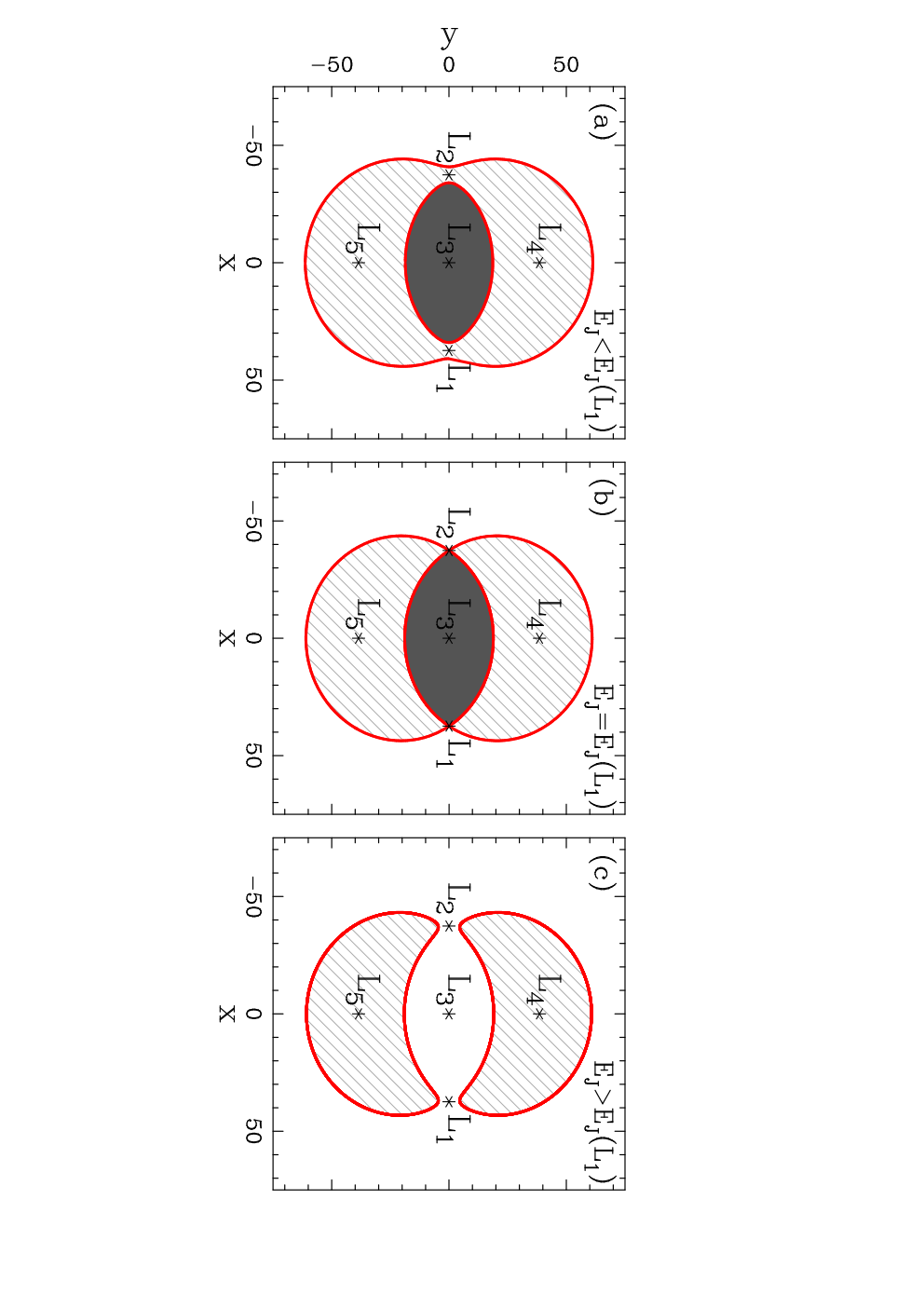
We choose a reference frame such that the origin of coordinates coincides with the centre of the galaxy and the triaxial system is fixed, i.e. a reference frame rotating with the system. The idea of the present analysis is based on the fact that if we consider a range of energies for which the particles are confined in the inner region defined by the zero velocity curve, in our case, for energies lower or equal to that of the unstable equilibrium points (), then there is no possible transfer of matter from the inner region of the galaxy to the outer region, or vice versa (see Fig. 1(a) and (b)). In this paper, we focus on energies slightly larger than that of the unstable equilibrium point, for which an opening in form of a bottleneck appears. We will hereafter refer to this aperture as bottleneck. Transfer of matter can be possible through this bottleneck (see Fig. 1(c)), and we study the objects that drive the motion in this region.
Therefore, our first goal is to study the neighbourhood of the unstable equilibrium points in the energy range where the bottleneck appears. This energy range is suitable to apply the normal form technique, which is known as the reduction to the centre manifold. As previously mentioned, it has been successfully applied to celestial mechanics problems, in particular to the Restricted Three Body Problem, e.g. [1, 3, 2]. The reduced Hamiltonian obtained from the reduction to the centre manifold process gives a good qualitative description of the phase space near the equilibrium points and uncouples the centre manifold from its hyperbolic behaviour. The procedure is similar to the Birkhoff normal form, usually used to study the stability properties around the central equilibrium point of the galaxy and to compute the families of periodic orbits around it, e.g. [12, 13, 14].
Our second goal is to study the behaviour of the hyperbolic invariant manifolds associated with the orbits contained in the centre manifold; these are essentially invariant manifolds of periodic orbits and invariant tori. As is well-known, stable and unstable invariant manifolds are dynamical features, that are responsible for the global dynamics in a dynamical system. In order to obtain the global picture of the transfer of mass, it is necessary to compute the invariant manifolds and to look for intersections between different parts, that is, obtaining the possible heteroclinic and homoclinic connections. These type of connections have been recently studied in the Restricted Three Body Problem and applied to obtaining transit and non-transit orbits in celestial mechanics [4, 5].
In Section 2, we describe the characteristics of the galactic model. In Section 3, we present the equations of motion and we study the effect of the main parameters on the linear behaviour of the equilibrium points. In Section 4, we explain in detail the reduction to the centre manifold in the particular case of the logarithmic potential and perform a study of the practical convergence of the reduced Hamiltonian. In Section 5, we compute the invariant manifolds associated with periodic orbits and quasi-periodic orbits and we study the role they play in the transfer of matter. We also perform an analysis on the variation of the free parameters of the potential. Finally, in Section 6 we conclude.
2 Galactic model
We consider a galactic model that fulfils the regularity requirements needed for the reduction to the centre manifold and that describes a triaxial system. We have selected the logarithmic potential [15], which is analytical and has the expression
| (1) |
The parameters and are non-dimensional constants that determine the shape of the potential, being the planar and the vertical axial ratios. Without loss of generality, we can consider the potential orientated such that . On the plane, higher values of represent more circular systems, independent of . Analogously, on the plane, higher values of represent more circular systems, independent of . For a standard triaxial figure, we choose and . The constants and simply set the scale for the velocity and length, respectively. The velocity corresponds to a circular asymptotic velocity at infinity and we consider , while when is different from zero, the singularity of the potential in the origin is avoided. We choose . The pattern speed is set to , characteristic for slow rotating systems [15]. The density associated with the potential is obtained via Poisson’s equation . The terms in the Laplacian equation associated with the and components are always positive, while the term associated with the -component can become negative for large values of . This introduces a restriction on the parameters and of the form . Throughout this paper we will use these standard values to fix the model and we will refer to it as “Model 1”. In the left panel of Fig 2, we show the isodensity contours of “Model 1”, and, in the right panel, the corresponding circular velocity curve, i.e. the velocity of a hypothetical star on a circular orbit. We note that we obtain elliptical isodensity contours and a flat rotation curve, these characteristics being appropriate for the study of triaxial systems.


3 Equations of motion and study of the linear stability of the unstable equilibrium points
As is usual in galactic models, we consider a Hamiltonian formulation that, in our case, has a Hamiltonian function given by:
where are the coordinate positions, are the associated conjugate momenta in a rotating reference frame, and is the angular velocity of the galaxy in the inertial system (for a more detailed explanation see Binney & Tremaine [15]). The equations of motion in Hamiltonian coordinates are
where , , and . The effective potential is defined as . The surface is called the zero velocity surface, and its cut with the plane is the zero velocity curve. All regions in which are forbidden to a star, so we call them forbidden regions (see Fig. 1).
As is well-known, the effective potential associated with the galactic model has five critical points, located in the -plane, where
Due to their similarity to the corresponding points in the Restricted Three Body Problem, they are often called Lagrangian points. and are located on the -axis symmetrically with respect to the centre, is placed at the origin of coordinates, and and are located on the -axis symmetrically with respect to the centre. The linearised motion around and is characterised by the superposition of a saddle behaviour in the -plane and two oscillations, one in-plane and one out-of-plane. Therefore, and are linearly unstable points and their behaviour is known as saddle centre centre. They are usually called the hyperbolic points. The linearised motion around , , and is characterised by the superposition of three oscillations, two in-plane and one out-of-plane. This behaviour is also known as a centre centre centre behaviour, so they are linearly stable and they are usually called the elliptic points.
3.1 Variation of the free parameters
As previously mentioned, we concentrate on energy levels slightly larger than the energies of the equilibrium points and . At these energies there is a bottleneck in the region between the two zero velocity curves and we want to know the type of orbits that transit through it.
The model parameters influence the global morphology, even for energy levels for which the bottleneck is open. Here we study the effect of the variation of the free parameters on the linear behaviour of the equilibrium points and . For this purpose, we fix the values of and , as in “model 1”, and study the influence of , , and , separately. We make families of models in which only one of the parameters is varied, while the others are kept fixed. For each of the models in the family, we study the linear behaviour of the equilibrium points . We expand the effective potential, , around one of these points and we retain only first order terms. For , the eigenvalues of the differential matrix corresponding to the planar motion are of the form: , , and those corresponding to the vertical motion of the form . Note that , and are positive in general non-equal real numbers. Therefore, is a linearly unstable saddle point, since the two real eigenvalues are related to the hyperbolic behaviour, while the purely imaginary are associated with the elliptic motion.
We first study the effect of the pattern speed, . We vary the value of within the range , the low values being characteristic for slow rotators and the large values, characteristic of fast rotators. In Fig. 3(a), we show how the modulus of the eigenvalues changes with the pattern speed. We observe that as the pattern speed decreases, the eigenvalues tend to zero, thus cancelling the hyperbolic character of and removing the possibility of having transit orbits. The pattern speed is, on the other hand, related to the position of the equilibrium points through the expression , where is the distance from the centre to and is the potential on the equatorial plane. As decreases, increases, so the equilibrium points move farther out from the centre. In Romero-Gómez et al. [6, 7], we consider a barred galaxy model, whose hyperbolic equilibrium points are in the vicinity of the bar ends, and we relate the spiral arms and rings in barred galaxies to the invariant manifolds of the periodic orbits around the hyperbolic equilibrium points. Elliptical galaxies, however, are considered to rotate very slowly or even not rotate [15, 16]. These triaxial systems have the equilibrium points too farther out and, according to our results, their hyperbolic character is cancelled. Thus, no transfer or escape of matter is possible, which is in agreement with observations because elliptical galaxies do not present spiral arms or rings.
In Fig. 3(b) we show the effect of the planar shape parameter, , on the eigenvalues of the differential matrix. We consider models where we vary in the range . We consider several models with different values of , limiting ourselves, for each value of , to models with a value satisfying the restriction , in order to avoid negative densities in the axis mentioned before. The value of is kept fixed as in “Model 1”. In all cases, as increases, the eigenvalues tend to decrease. In particular, the real eigenvalue, , tends to zero thus cancelling the hyperbolic character of the points. However, note that, as expected, for a fixed value of (vertical axial ratio), the corresponding vertical eigenvalue, , does not change as we vary (planar axial ratio). A similar behaviour can be observed in Fig. 3(c), where we study the effect of the vertical shape parameter, . The eigenvalues tend to decrease as the vertical axial ratio increases. However, for a fixed value of the planar axial ratio, , the values of and remain constant. Therefore, we can conclude that only the shape parameter has an influence on the planar structure of the galaxy, while the parameter will influence the vertical behaviour.


In conclusion, the hyperbolic character of and is, as expected, weaker for slowly rotating systems or for near-axisymmetric ones, e.g elliptical galaxies. The hyperbolic character is strong and the bottleneck is open to global structures, in the opposite cases, e.g. bars.
4 Reduction to the centre manifold
The reduction to the centre manifold is a suitable tool for studying the neighbourhood of the hyperbolic equilibrium points. It was first introduced in Gómez et al. [1] for the Restricted Three Body Problem and further detailed in Gómez et al. [3]. The procedure can be summarised in two steps. First, the Hamiltonian function is expanded in power series around the equilibrium point. Then, a partial normal form scheme is applied in order to uncouple (up to a high order) the hyperbolic directions from the elliptic ones. Now the truncated Hamiltonian has an invariant manifold tangent to the elliptic directions of the linear part. The restriction to the invariant manifold tangent to the elliptic directions leads to a Hamiltonian system with two degrees of freedom and an elliptic equilibrium point at the origin. This restriction to the manifold is the so-called reduction to the centre manifold and the study of the dynamics of the reduced Hamiltonian gives a qualitative description of the phase space near the equilibrium point.
We want to note here that we do not use the Birkhoff Normal Form (hereafter, BNF). We are interested in performing a local study of a hyperbolic equilibrium point in the largest region possible. In that sense, the reduction to the centre manifold can provide better results in a larger neighbourhood than BNF. Furthermore, as we will see in Section 5, we are interested in computing the invariant manifolds associated with periodic orbits and quasi-periodic orbits and the normal form described here provides as well initial conditions to compute both invariant objects.
We proceed by first obtaining the quadratic real normal form of the second order term of the Hamiltonian function. This is achieved by performing two changes of coordinates. The first one consists of a translation plus an homothecy in order to place the new origin of coordinates on the equilibrium point and to set the unit length equal to the distance from the equilibrium point to the origin. The second change of variables allows us to write the second order part of the Hamiltonian in its real normal form. We then perform a complexification of the variables, in order to obtain a Hamiltonian of diagonal form. Finally, the normal form of higher order terms is computed. In the following subsections, we describe in detail the steps performed and in the last subsection we study the practical convergence of the reduced Hamiltonian.
4.1 Translation and homothecy
As previously mentioned, the first change of coordinates consists of a translation plus an homothecy. The translation sets the new origin of coordinates on any of the symmetric hyperbolic equilibrium points and the homothecy sets the unit of distance as the distance from the origin of the old system to the position of the equilibrium point. Furthermore, the change has to be symplectic, i.e. it must preserve the Hamiltonian equations in the new variables.
If we write as the
Hamiltonian barycentric coordinates and
as the
Hamiltonian ones around the hyperbolic equilibrium point, the symplectic change can be
written as:
where are the coordinates of the hyperbolic equilibrium point and . Expanding the logarithmic potential up to second order, the expression for the Hamiltonian in the new coordinates around , is
where is a constant and .
4.2 The quadratic real normal form
The second change of coordinates will express the second order term of the Hamiltonian in its real normal form . This is accomplished via a linear and symplectic change performed around the hyperbolic equilibrium point . The analysis for is analogous and the results are symmetric.
For , we have
and .
We note that the planar motion is uncoupled from the vertical motion, so we perform the reduction to the real normal form in two steps, that is, first regarding the in-plane motion and then the out-of-plane motion. In the 2D case, the differential matrix around becomes
where
The matrix has two real, , and two purely imaginary, , eigenvalues. The eigenvectors associated with the real eigenvalues have the following expression
| (2) |
while the eigenvector associated with the imaginary eigenvalue is
Considering , where , we obtain the suitable scaling factors and that give the final symplectic change of variables regarding the in-plane motion:
Regarding the out-of-plane motion, the symplectic transformation is given by
where always. The final change of coordinates sets the Hamiltonian around the equilibrium point with coordinates that express the second order term in its real normal form. That is, after performing the second change of coordinates, the second order term of the Hamiltonian is:
| (3) |
For subsequent computational purposes, it is desirable to work with complex variables. Then, a third change of variables is needed in order to write the second order term of the Hamiltonian in the complex diagonal normal form.
4.3 Complexification
We are interested in writing the second order Hamiltonian in a diagonal form, in order to simplify the homologic equation that we encounter in the normal form process. We perform a complexification of the variables related to and . That is, we perform a symplectic change of coordinates from real coordinates to complex coordinates of the normal form complexifying the pairs and by means of:
In this way, the second order Hamiltonian has the form:
| (4) |
where , and are real positive numbers.
4.4 Normal form of higher order terms
We have now written the second order term of the Hamiltonian, , in its real and in its complex normal form. The final step to obtain the centre manifold consists of removing some monomials in the expansion of the Hamiltonian so that the final Hamiltonian has an invariant manifold tangent to the elliptic directions of . We apply the method known as the Lie Series method (see [2, 3] and references therein for a detailed description in the Restricted Three Body Problem). Until the end of this section, we use the following notation. If is a vector of complex numbers and is an integer vector, we denote the term and in this context we define as . We define as .
The initial Hamiltonian is expanded around the hyperbolic equilibrium point in the complex coordinates for which the second order term is in diagonal form (Eq. 4). Thus, the Hamiltonian11 1 Bold letters denote vector notation. has the form
where is given as in Eq. 4 and is a homogeneous polynomial of degree of the form , where denotes .
The Poisson bracket of two functions, and , of position and momenta is defined as
If and are homogeneous polynomials of degree and respectively, then is a homogeneous polynomial of degree . If a function is considered a Hamiltonian then, the function defined by
is the result of applying a time one map canonical transformation under the flow of to the Hamiltonian . The Hamiltonian is usually called the generating function. If we choose a homogeneous polynomial of degree 3, , as a generating function, then the homogeneous polynomials of degree , , such that are given by
In order to remove all the terms of order three in the new Hamiltonian, i.e. to have , we must choose a generating function, , such that it solves the homological equation . This procedure can be used recurrently trying to find homogeneous polynomials to remove non-resonant terms of the Hamiltonian.
In our case, we are interested in removing the instability associated with the hyperbolic character of the Hamiltonian . We note that the second order term of the Hamiltonian provides the linear part of the Hamiltonian equations. Therefore, the instability is associated with the term . For the linear approximation of the Hamiltonian equations, the centre part can be obtained by setting . If we want the trajectory to remain tangent to this space (i.e. to have for all ), then we need when adding the nonlinear terms. Due to the autonomous character of the Hamiltonian system, we will obtain for all . We remember that the Hamiltonian equations associated with a Hamiltonian are
In particular,
Therefore, we can obtain the required condition, when , if in the expansion of the Hamiltonian there are no monomials with exponents and . Different changes of variables can be used for such purpose, the most common being the ones cancelling the terms with [3] or cancelling only terms with . This second choice cancels the minimum number of terms in the Hamiltonian and is the one we have chosen in this paper.
Thus, after the final change of variables the Hamiltonian can be written in the form:
where is a polynomial of degree without terms of and is a remainder of order , which is very small near .
Finally, using the inverse change of variables of the complexification, the truncated Hamiltonian, can be expanded in real form and we obtain
where the second order term is as in Eq. 3.
4.5 Practical convergence
In order to check the practical convergence of the truncated series, we integrate the same initial condition on the centre manifold using both the reduced Hamiltonian up to order and the Hamiltonian in barycentric coordinates. At each time step, we compare the two position vectors by computing the norm of the difference. When this becomes greater than a given tolerance, we plot the initial condition and the time step it has reached. In Fig. 4, we show the practical convergence plots for four different energy levels and a tolerance of for “model 1”. In Fig. 5, we plot the energy levels for the same model but with a tolerance of . The energy of the equilibrium point is . In each panel, we consider an energy level higher than the previous one and initial conditions on the centre manifold. We note that, due to the energy confinement, the initial conditions valid for a given energy level lie inside the planar Lyapunov orbit. As the energy increases, the time, , at which the differences become greater than the tolerance, decreases. This is reflected in Figs. 4 and 5 by the colour palette. In all panels, the colour palette ranges from to , the green colour being associated with large times and the red colour, to small times. In Fig. 4, where we use as tolerance, we note that in the top left panel, the dominating colour is green, while as we increase the energy, the colours tend to yellow and red. We also observe that, as expected, as the tolerance decreases, the time also decreases, so in the bottom right panel of Fig. 5 the region is practically all orange and red.


Note that for a tolerance of , the practical convergence of the normal form is good for a wide range of energies, as all panels in Fig. 4 are basically green. Even for a more restrictive tolerance, , the normal form gives good results for a considerably range of energies, see top panels of Fig. 5. Also note that the numerical test we use here integrates initial conditions using both the reduced and the initial Hamiltonian. Since the initial Hamiltonian contains the instability, that grows exponentially in time, the time estimations we show here underestimate the real values of for which the reduced Hamiltonian gives accurate results.
5 Invariant objects around . Transfer of matter
In the following, we apply the methodology introduced in the previous section to compute the invariant manifolds associated with both periodic orbits and invariant tori. We fix the values of the potential and study the neighbourhood of the hyperbolic equilibrium point . We first compute the invariant curves around the equilibrium point on the section given by and within a range of energies. We then compute the invariant manifolds of the planar and vertical Lyapunov orbits and of the invariant tori. We also study the role invariant manifolds of periodic orbits have in the transfer of matter in the galaxy by computing the homoclinic and heteroclinic connections between the periodic orbits of a given energy level. Finally, we study the variation of the free parameters and check their influence on the presence of homoclinic and heteroclinic orbits, thus, on the global shape produced by the invariant manifolds.
5.1 Invariant manifolds of periodic orbits and quasi-periodic orbits
Throughout this section we fix the model parameters to those of the standard “model 1” and we compute the invariant objects using the Hamiltonian in the normal form up to order in the reduced coordinates. For clarity of the representation, however, at each step we perform the backwards change of variables to plot the results in the initial frame using barycentric coordinates.
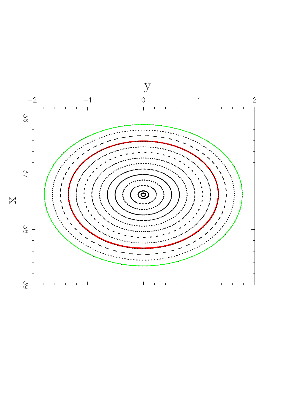
We compute the invariant curves on the section and the planar Lyapunov orbit surrounding the equilibrium point, see top panel of Fig. 6. To obtain the invariant curves, we take initial conditions on the galactic plane of the initial frame of reference and we plot the cuts with the section. Each invariant curve on the section represents an invariant torus, as is shown in the top and bottom left panels of Fig. 6. In the bottom left panel, we plot the invariant torus corresponding to the invariant curve on the section (red solid line) in the original coordinates, although the numerical integration is performed using the reduced Hamiltonian. Since the reduced Hamiltonian has the hyperbolic component decoupled from the elliptic one, we can perform long time integrations without the instability. For convenience, however, we use the normal form change of variables at each integration step to display the orbits in the original coordinates. In the bottom right panel, we plot the vertical Lyapunov orbit. We observe that for the range of energies for which the normal form of the Hamiltonian is accurate, the section of the invariant curves has always the same aspect, i.e., the only macroscopic objects we see are the Lyapunov orbits and invariant tori.


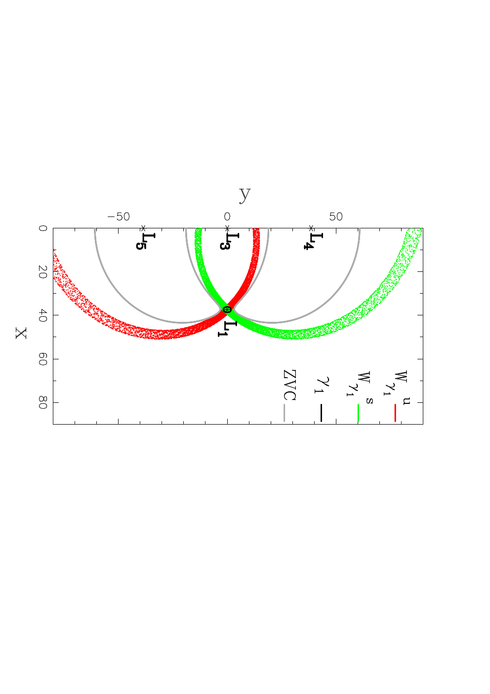
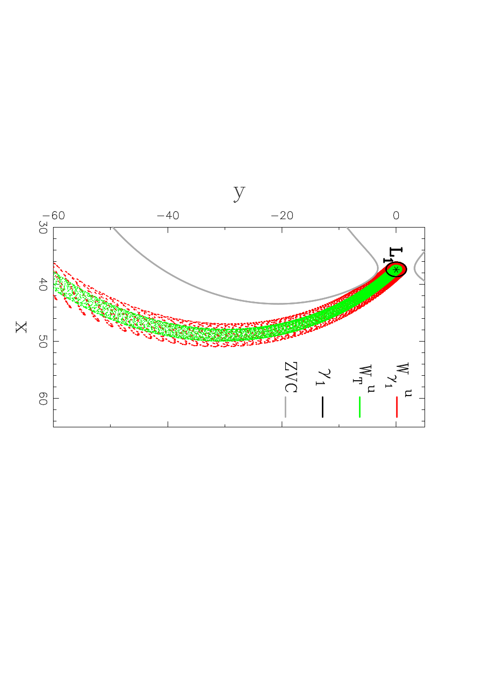
We can also compute the hyperbolic invariant manifolds associated with the planar and vertical Lyapunov orbits and with the invariant tori. We first compute the stable and unstable invariant manifolds associated with the planar Lyapunov periodic orbit around the equilibrium point , and respectively, using the truncated Hamiltonian up to order . According to the normal form scheme used, the initial conditions approximating the unstable invariant manifold of a planar Lyapunov orbit have the form and the initial conditions for the stable invariant manifold are . Note that invariant manifolds are sets of asymptotic orbits that tend to and depart from the periodic orbit. In the left panel of Fig. 7, we plot and for the energy level () and . We also plot the zero velocity curve defining the forbidden region. Here we observe the characteristic saddle behaviour of the invariant manifolds due to the hyperbolic behaviour of the periodic orbit. Also note that the invariant manifolds connect the inner region with the outer region, in the sense that the existence of invariant manifolds of periodic orbits implies also the existence of transit orbits between the two regions delimited by the zero velocity curves. In the right panel of Fig. 7, we plot the unstable invariant manifold of an invariant torus for the energy level . The initial conditions to compute the unstable and stable invariant manifolds of invariant tori are easily provided by the normal form we use. That is, for the unstable manifold, for the stable manifold and . We superimpose it to the unstable invariant manifold of the planar Lyapunov orbit of the same energy and we observe that they describe approximately the same loci in the -projection, the invariant manifold of the invariant torus being located inside the invariant manifold of the planar periodic orbit.
In Fig. 8, we plot the unstable invariant manifolds of both the planar, , and vertical, , Lyapunov orbits of the same energy level (). The initial conditions used to compute the unstable invariant manifold of the vertical Lyapunov orbit have the form and the initial conditions for the stable invariant manifold are , with . In the left panel, we plot the invariant manifolds on the projected galactic plane. We observe that they both describe essentially the same loci, the invariant manifold of the vertical Lyapunov orbit being located inside the invariant manifold of the planar Lyapunov orbit in the configuration space. In the right panel, we show the three dimensional view of the same manifolds. We observe that the invariant manifolds of the planar Lyapunov orbits drive the motion dominating over the invariant manifolds of the vertical Lyapunov orbits. This is due to the fact that the unstable component lies within the plane, since the two real eigenvalues are associated with the in-plane motion. We can, therefore, conclude that the motion in the neighbourhood of and is basically dominated by the invariant manifolds of planar periodic orbits.


5.2 The role of invariant manifolds in the transfer of matter
As we have seen, the motion in a neighbourhood of a hyperbolic point is mainly driven by the invariant manifolds of planar periodic orbits, so in this section we restrict ourselves to the plane. The next step is to study the global behaviour of the invariant manifolds associated with planar periodic orbits and determine their role in global structures. In particular, we are interested in knowing whether the invariant manifolds can drive particles from the neighbourhood of to the neighbourhood of or even connect the neighbourhood of with itself using long-time trajectories. For clarity, as we did in previous sections, we plot the Poincaré maps and the orbits in the initial frame using barycentric coordinates.
A particle will be transferred from the vicinity of one Lagrangian point to the vicinity of the symmetric point if it is “trapped” first by and then by . To study these type of transitions, we use Poincaré surfaces of section, that is, we draw the crossings of trajectories through a particular plane or surface in phase space. Depending on the purposes of our study, some surfaces will be more suitable than others, but the methodology is the same. Let us take as an example the surface of section defined by with ; that is, we consider the orbits when they cut the plane having a positive value for the coordinate. Let us consider this surface of section for the stable and unstable invariant manifolds of a Lyapunov orbit around (located in the side). Taking initial conditions on the manifold and integrating forward in time (resp. backwards in time) until the first encounter with , we obtain the simple closed curves (resp. ) that can be seen in Fig. 9a. Although the simple closed curves and are obtained as the natural result of intersecting the manifold tubes with a plane, it should be mentioned that further crossings (i.e. and with ) may well not have this simple structure, as can be seen in the Restricted Three Body Problem example provided by Gidea and Masdemont [17].
In the selected example, and are represented in coordinates. It is important to note that a pair in defines an orbit in a unique way, since and is obtained from the energy level under study and in the sense of crossing . By definition of invariant manifold, a point in (black dots in Fig. 9a) represents a trajectory asymptotic to the Lyapunov orbit around both forward and backward in time and this trajectory is called a homoclinic orbit. In general, homoclinic orbits correspond to asymptotic trajectories, , such that . Thus, a homoclinic orbit departs asymptotically from the unstable Lyapunov periodic orbit around and returns asymptotically to it, as can be seen in Fig. 9b.

Heteroclinic orbits, on the other hand, are defined as asymptotic trajectories, , such that . Thus, a heteroclinic orbit departs asymptotically from the periodic orbit around and asymptotically approaches the corresponding Lyapunov periodic orbit of the same energy around the Lagrangian point at the opposite end of the bar region , ; a suitable surface of section, , for this computation can be the plane with . We hereafter refer to interior region as the elliptical-like shape defined by the iso-effective potential curves encircling the centre and roughly passing through and . In Fig. 10a, we plot the closed curves and on the surface . Note that there are two intersection points, therefore this model presents two heteroclinic orbits that will connect asymptotically one side of the interior region with the opposite, as can be seen in Fig. 10b.

The existence of these type of connections determines the way matter is transferred within the galaxy. By definition, if there are heteroclinic connections, they create a tube, where particles can be trapped and travel from one side of the interior region to the opposite. The intersection of the tube with the section can be seen in Fig. 10a as the hatched area obtained from intersecting the curves and . The global morphology in such models is reminiscent of that of rings [18, 6, 7]. rings are outer rings in barred galaxies whose semi-major axis is perpendicular to the one of the bar. They have a characteristic or -shape (see Fig. 11a). If the model presents homoclinic connections, particles can be trapped in tubes travelling from one end of the interior region to itself. The global morphology in this case is reminiscent of that of rings [18, 7] (see Fig. 11c). ringed galaxies present two outer rings, namely the ring previously mentioned and an ring, whose semi-major axis is parallel to the bar semi-major axis (see Fig. 11b). Note that if neither heteroclinic nor homoclinic connections exist, particles are not able to return to the vicinity of the interior region in an early stage. Thus the particles follow an escaping trajectory forming spiral arms [7] (see Fig.11d).


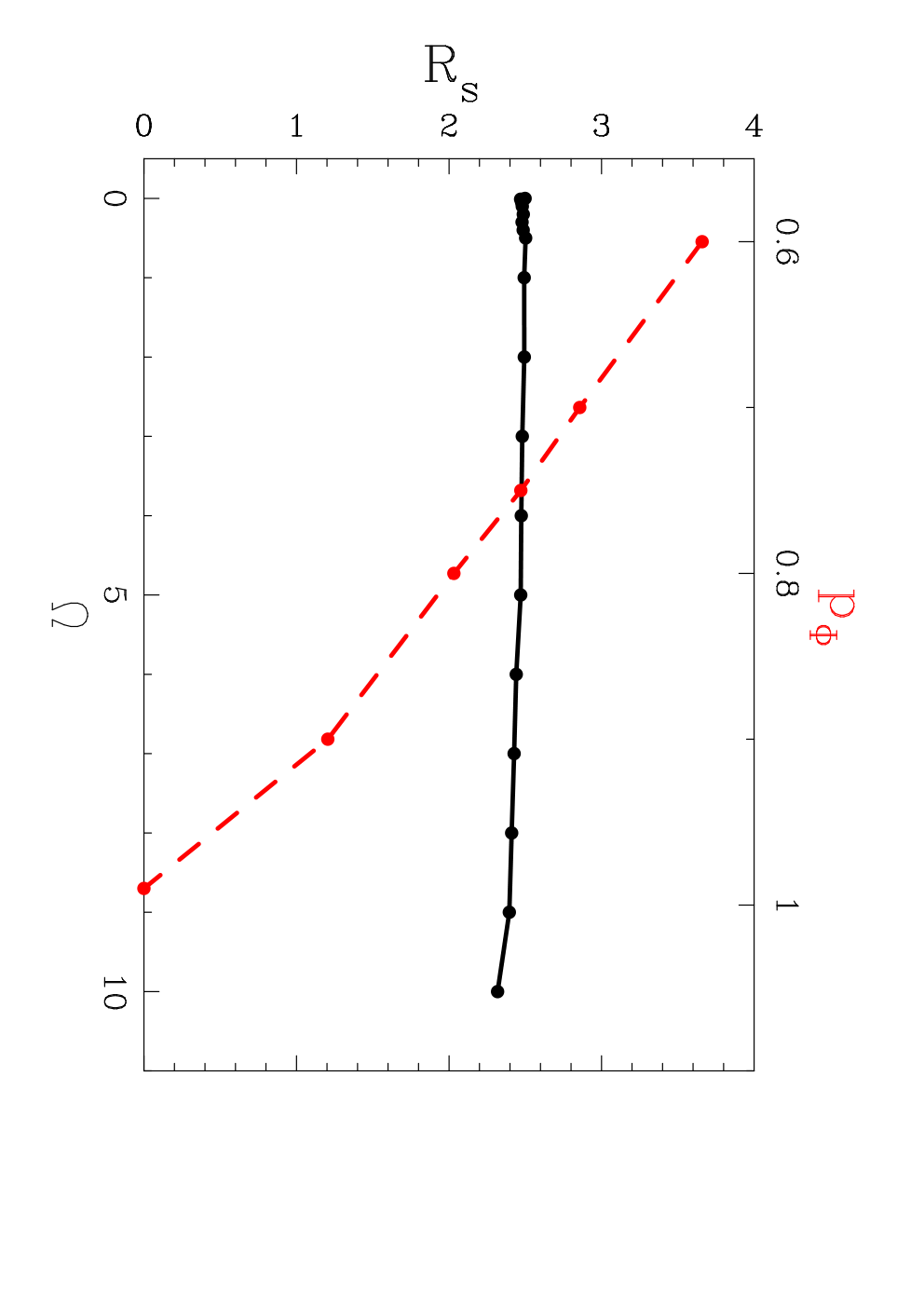
In Sect. 5.1 we show that motion is mainly driven by the invariant manifolds of the planar Lyapunov orbits. Here we follow the study in Sect. 3.1 and we compute the invariant manifolds of families of models where we vary the pattern speed, , and the planar axial ratio, , i.e. the two dynamical parameters that have an effect on the potential in the galactic plane. The rest of the parameters are fixed as in “model 1”. For each model, we compute the family of planar Lyapunov orbits in a range of energies for which they are unstable and the bottleneck through the zero velocity curve is opened. We compute the invariant manifolds associated with the planar periodic orbits and we study the existence of possible heteroclinic and homoclinic connections. In each panel of Fig. 12, we plot the corresponding global morphology. In the left column we increase from top to bottom the value of the pattern speed. In all cases the global shape of the invariant manifolds is two spiral arms and the degree of openness is essentially independent of the value of the pattern speed. This can be seen in Fig. 13, where we plot a measure of the openness of the spiral, namely the ratio, , between the -coordinate of the outer branch of the unstable invariant manifold at the first cut with the axis and the absolute value of -coordinate of the equilibrium point. In the right column of Fig. 12, we plot the invariant manifolds for models with different values of . When the system is strongly non-axisymmetric, no homoclinic or heteroclinic connections are present and the global structure is that of two spiral arms. When , the model presents homoclinic connections with both ends of the interior region. As previously mentioned, the global morphology reminds that of rings. As approaches to , that is, the system becomes prolate, the invariant manifolds tend to close, heteroclinic connections are present and the structure forms an ring. We stress the similarity of these patterns with the schematic prototypes of outer rings described by Buta & Crocker [18]. In Fig. 13, we also plot the degree of openness as the shape parameter varies. As is illustrated in the right column of Fig. 12, the value of the ratio decreases as the value of approaches to .

6 Conclusions
In this paper we use a suitable galactic potential (the logarithmic potential) to perform a semi-analytic study of the neighbourhood of the unstable equilibrium points and . For a detailed study of their neighbourhood, we use a partial normal form scheme and we find that the main objects are the planar and vertical families of Lyapunov orbits and invariant tori. We compute the invariant manifolds associated with both periodic orbits and quasi-periodic orbits using the reduced Hamiltonian and we find that the motion around and is mainly driven by the invariant manifolds of the planar Lyapunov orbits. However, we are also interested in the global structure of the galaxy. Thus, we study the possible homoclinic and heteroclinic connections between the planar periodic orbits. For such a purpose, we use suitable Poincaré surfaces of section. We note that this approach has successfully been used in celestial mechanics and in this paper we apply it to a galactic dynamics problem, namely the formation of spiral arms and rings in barred galaxies, in comparison to other theories given so far.
Here we are interested in the hyperbolic behaviour of and and, particularly, in determining the role the invariant manifolds play in the transfer of matter for energy levels where the zero velocity curves are open (i.e. a range of energies somewhat larger than the energy of and ) and a bottleneck appears around and . For such purpose, we also study the influence of the main model parameters, namely the pattern speed, , and the shape parameters, and . The logarithmic models are suitable for describing triaxial systems such as haloes, bars, bulges in disc galaxies or elliptical galaxies. The structures we have constructed using the invariant manifolds, however, are not globally dependent on the model characteristics [6, 7]. This implies, for example, that if a system had some degree of rotation, these kind of structures should be present. Elliptical galaxies are triaxial systems that do not present any external feature, i.e. they are an ellipsoidal distribution of matter with different degrees of ellipticity and they present neither spiral arms nor rings. Observations show that elliptical galaxies barely rotate or do not rotate at all as a figure [15, 16]. Our results are in agreement with this statement. We have shown that models that rotate slowly or do not rotate cancel the hyperbolic behaviour of the equilibrium points and, thus, no transfer or escape of matter is possible. On the other hand, bars in disc galaxies are non-axisymmetric components usually characterised in the literature by elliptical distributions of density [19] although both observations and simulations show they might have more rectangular endings [20, 21]. It is well-known that bars rotate and observations show that spiral arms or rings emanate from the ends of the bar. This characteristic is also consistent with our results which show that if the system rotates at a given angular velocity, the hyperbolic equilibrium points are present, so that the invariant manifolds drive the motion, and therefore, set the global morphology to the galaxy. We have seen that, depending on the rotation velocity and the shape of the bar, the morphology will be that of a barred spiral galaxy or that of a barred ringed galaxy.
Acknowledgements
This work partially supported by the Spanish grants MCyT-FEDER MTM2006-00478 and AYA2007-60366 and the French grant ANR-06-BLAN-0172. MRG acknowledges her “Becario MAE-AECI” and the Marie Curie Research Training Network Astronet.
References
- (1) Gómez, G., Jorba, A., Masdemont, J.J., & Simó, C., Study refinement of semianalytical halo orbit theory, ESOC Contract 8625/89/D/MD(SC), Final Report, 1991.
- (2) Jorba, A., & Masdemont, J., Dynamics in the centre manifold of the collinear points of the restricted three-body problem, Physica D 132 (1999) 189-220.
- (3) Gómez, G., Jorba, A., Masdemont, J.J., & Simó, C., Dynamics and Mission Design near Libration Points. Advanced Methods for Collinear Points, Volume 3, World scientific, Singapore, 2001
- (4) Koon, W.S., Lo, M.W., Marsden, J.E., & Ross, S.D., Heteroclinic connections between periodic orbits and resonance transitions in celestial mechanics, Chaos 10, No.2 (2000) 427-461.
- (5) Gómez, G., Koon, W.S., Lo, M.L., Marsden, J.E., Masdemont, J.J., & Ross, S.D., Connecting orbits and invariant manifolds in the spatial restricted three-body problem, Nonlinearity 17 (2004) 1571-1606.
- (6) Romero-Gómez, M., Masdemont, J., Athanassoula, E., & García-Gómez, C, The origin of ring structures in barred galaxies, Astronomy and Astrophysics 453 (2006) 39-45.
- (7) Romero-Gómez, M., Athanassoula, E., Masdemont, J., & García-Gómez, C, The formation of spiral arms and outer rings in barred galaxies, Astronomy and Astrophysics 472 (2007) 63-75.
- (8) Athanassoula, E., Romero-Gómez, M., & Masdemont, J.J., (2008) in preparation.
- (9) Lindblad, B., On the possibility of a quasi-stationary spiral structure in galaxies, Stockholms Observatorium Ann. 5 (1963) 1-20.
- (10) Toomre, A., Group velocities of spiral waves in galactic disks, The Astrophysical Journal 158 (1969) 899-913
- (11) Athanassoula, E., The spiral structure of galaxies, Physics reports 114 (1984), 319-403.
- (12) Gustavson, F.G., On Constructing Formal Integrals of a Hamiltonian System Near an Equilibrium Point, The Astronomical Journal 71 (1966) 670-686.
- (13) Miralda-Escudé, J, & Schwarzschild, M., On the orbit structure of the logarithmic potential, The Astrophysical Journal 339 (1989) 752-762.
- (14) Belmonte, C., Boccaletti, D., & Pucacco, G., On the orbit structure of the logarithmic potential. The Astrophysical Journal 669 (2007) 202-217.
- (15) Binney, J., & Tremaine, S., Galactic Dynamics, Princeton University Press, New Jersey, 1987.
- (16) Schwarzschild, M., Triaxial equilibrium models for elliptical galaxies with slow figure rotation, The Astrophysical Journal 263 (1982) 599-610.
- (17) Gidea, M., & Masdemont, J.J., Geometry of homoclinic connections in a planar circular Restricted Three Body Problem, International Journal of Bifurcation and Chaos 17 (2007) 1151-1169.
- (18) Buta, R., & Crocker, D.A., The outer Lindblad resonance and the morphology of early type disk galaxies, The Astronomical Journal 102 (1991) 1715-1723.
- (19) Pfenniger, D., The 3D dynamics of barred galaxies, Astronomy and Astrophysics 134 (1984) 373-386
- (20) Athanassoula, E., Morin, S., Wozniak, H., Puy, D., Pierce, M.J., Lombard, J., & Bosma, A., The shape of bars in early-type barred galaxies, Monthly Noticies of the Royal Astronomical Society 245 (1990) 130-139
- (21) Athanassoula, E., & Misiriotis, A., Morphology, photometry and kinematics of N-body bars - I. Three models with different halo central concentrations, Monthly Noticies of the Royal Astronomical Society 330 (2002) 35-52