Baryogenesis via Leptogenesis in Adjoint SU(5)

The origin of the baryon asymmetry in the Universe is one of the most interesting issues in modern cosmology. One of the simplest explanations is provided by the Baryogenesis via Leptogenesis scenario [1], where the lepton asymmetry generated in the out-of-equilibrium decays of the fields responsible for the seesaw mechanism of neutrino masses [2] is converted into a baryon asymmetry by sphaleron transitions [3]. This idea is very appealing due to the strong connection with the origin of neutrino masses.

Grand Unified Theories (GUTs) [4] are one of the most appealing extensions of the Standard Model (SM), explaining e.g. the origin of the SM gauge interactions and neutrino masses. In particular, these theories provide a natural framework for the implementation of the Baryogenesis via Leptogenesis mechanism mentioned above. In this article we study the leptogenesis mechanism and its possible predictions in the context of the Adjoint $SU(5)$ [5]. In this theory the Higgs sector is composed of $\bm{5_{H}}$, $\bm{24_{H}}$ and $\bm{45_{H}}$ Higgses and the matter lives in the $\bm{\bar{5}}$, $\bm{10}$, and $\bm{24}$ representations. All fermion masses are generated at the renormalizable level, and neutrino masses are generated through the Type I and Type III [6] seesaw mechanisms. The predictions coming from the unification of gauge interactions and proton decay were studied in great detail in [7], where the authors concluded that the lightest fermionic field living in the adjoint representation has to be the field responsible for the Type III seesaw mechanism. This result strongly motivates us to study the leptogenesis mechanism in the context of Adjoint $SU(5)$ since in this case there is no ambiguity about which field is responsible for leptogenesis.

Our first finding is that the $C\!P$ asymmetry is generated only by the vertex correction since the self-energy contribution vanishes. When the neutrino mass hierarchy is normal, successful leptogenesis is possible in a large region of the parameter space. On the contrary, when the spectrum for neutrinos is inverted, we find consistent solutions for a very restricted mass range. Finally, we show that imposing the constraints coming from leptogenesis one can rule out a large region in the parameter space of the theory which was allowed by the unification of gauge interactions and the constraints coming from proton decay.

The paper is organized as follows: In Section II we discuss the theory of Adjoint $SU(5)$ and its predictions for neutrino masses. In Section III we present our computation of the baryon asymmetry through leptogenesis, and derive bounds on the mass of the field responsible for the Type III seesaw. In Section IV we discuss the possible constraints on the spectrum of the theory from successful leptogenesis. In the last section we summarize our main results.

In the context of Adjoint $SU(5)$ [5] neutrino masses are generated through the Type I [2] and Type III [6] seesaw mechanisms. In this theory the Higgs sector is composed of $\bm{5_{H}}$, $\bm{24_{H}}$, and $\bm{45_{H}}$ and the matter fields live in ${\bf{\bar{5}}}=(d^{C},l)_{L}$, ${\bf{10}}=(u^{C},Q,e^{C})_{L}$ and ${\bf{24}}=(\rho_{8},\rho_{3},\rho_{(3,2)},\rho_{(\bar{3},2)},\rho_{0})_{L}=({8},{1},0)\bigoplus({1},{3},0)\bigoplus({3},{2},-5/6)\bigoplus(\overline{{3}},{2},5/6)\bigoplus({1},{1},0)$. In our notation $\rho_{3}$ and $\rho_{0}$ are the $SU(2)_{L}$ triplet responsible for Type III seesaw and the singlet responsible for Type I seesaw, respectively. See reference [8] for the supersymmetric version of the theory.

The relevant interactions for neutrino masses in this context are given by:

where $\alpha=1,2,3$, and $H_{1}$ and $H_{2}$ are the Higgs doublets living in ${\bm{5_{H}}}$ and ${\bm{45_{H}}}$, respectively. Once $\bm{24_{H}}$ gets the expectation value, $\langle\bm{24_{H}}\rangle=v\,{\rm diag}(2,2,2,-3,-3)/\sqrt{30}$, the masses of the fields responsible for seesaw living in $\bm{24}$ are given by:

where we have used the relations $M_{V}=v\sqrt{5\pi\alpha_{\rm GUT}/3}$, $\tilde{\lambda}=\lambda/{\sqrt{50\pi}}$ and chose $M_{V}$ as the unification scale. The predictions coming from the unification of gauge interactions and proton stability was studied in detail in [7]. In this recent study the authors concluded that in order to satisfy the unification and proton decay constraints the field $\rho_{3}$ has to be the lightest field in the $\bm{24}$ representation. Therefore, the theory [5] is a good theory for leptogenesis since one can predict which field generates the lepton asymmetry.

Once the GUT symmetry is broken by the vev of $\bm{24_{H}}$, all elements of the mass term for the Higgs doublets are large, of order the GUT scale. Diagonalizing the mass matrix, one obtains one light eigenstate, to be identified with the SM Higgs $H$, and one heavy eigenstate $H^{\prime}$ with a mass at the GUT scale. In particular, it is relevant for our study that $\rho_{3}$ is only kinematically allowed to decay into the SM Higgs $H$.

Writing $H_{1}=\cos\alpha\ H\ -\ \sin\alpha\ H^{\prime}$ and $H_{2}=\sin\alpha\ H\ +\ \cos\alpha\ H^{\prime}$, and since only $H$ gets a vev $\langle H\rangle=v_{0}/\sqrt{2}$, we have that $\cos\alpha=v_{5}/v_{0}$ and $\sin\alpha=v_{45}/v_{0}$. The relevant terms in Eq. (1) with the addition of the mass terms are then given by

where¹¹ 1 Compared to [5] we use the more convenient definition in the context of leptogenesis $a_{\alpha}\equiv h_{\alpha 1}$ and $b_{\alpha}\equiv h_{\alpha 2}$, which makes apparent the similarity between the model under consideration and the type I seesaw model with two right-handed neutrinos.

with $v_{0}=174~{\rm GeV}$. In the above equations $v_{5}/\sqrt{2}=\langle\bm{5_{H}}\rangle$, $v_{45}/\sqrt{2}=\langle\bm{45_{H}}\rangle^{15}_{1}=\langle\bm{45_{H}}\rangle^{25}_{2}=\langle\bm{45_{H}}\rangle^{35}_{3}$, and the matrix representation for $\rho_{3}$ is given by

Integrating out the fields responsible for the seesaw mechanism, the mass matrix for neutrinos reads as

The theory [5] predicts one massless neutrino at tree level. Therefore, we could have either a normal neutrino mass hierarchy: $m_{1}=0$, $m_{2}=\sqrt{\Delta m_{\rm sol}^{2}}$ and $m_{3}=\sqrt{\Delta m_{\rm sol}^{2}+\Delta m_{\rm atm}^{2}}$, or the inverted neutrino mass hierarchy: $m_{3}=0$, $m_{2}=\sqrt{\Delta m_{\rm atm}^{2}}$ and $m_{1}=\sqrt{\Delta m_{\rm atm}^{2}-\Delta m_{\rm sol}^{2}}$. $\Delta m_{\rm sol}^{2}\simeq 8\times 10^{-5}$ eV² and $\Delta m_{\rm atm}^{2}\simeq 2.5\times 10^{-3}$ eV² are the mass-squared differences of solar and atmospheric neutrino oscillations, respectively [9].

Finally, the kinetic terms for the fields responsible for seesaw read as

where $D_{\mu}\ \rho_{3}=\partial_{\mu}\rho_{3}\ +\ {\rm i}g_{2}\ [W_{\mu},\rho_{3}]$ and

The gauge-scattering term coming from the kinetic term will be crucial in the leptogenesis analysis, which we will be dealing with in the next section. A convenient parametrization of the $3\times 2$ Yukawa coupling matrix $h$ is the so-called Casas-Ibarra [10]

where $U$ is the PMNS lepton mixing matrix, $D_{\nu}={\rm diag}(m_{1},m_{2},m_{3})$ and $D_{\rho}={\rm diag}(M_{\rho_{3}},M_{\rho_{0}})$. The $\Omega$ matrix takes here the well-known form corresponding to the Type I seesaw case with 2 right-handed neutrinos [11]:

in the normal and inverted hierarchy, respectively, and where $\omega$ is a complex parameter. $\xi=\pm 1$ is a discrete parameter that accounts for a discrete indeterminacy in $\Omega$. For the PMNS matrix $U$, we adopt the usual parametrization [12]

where $s_{ij}\equiv\sin\theta_{ij}$, $c_{ij}\equiv\cos\theta_{ij}$, $\delta$ is the Dirac $C\!P$-violating phase, $\Phi$ is a Majorana $C\!P$-violating phase. Neglecting statistical errors, we will use throughout our study the values $\theta_{12}=\pi/5$ and $\theta_{23}=\pi/4$, compatible with the results from neutrino oscillation experiments. Moreover, we will adopt the $3\sigma$ range $s_{13}=0\textrm{--}0.20$.

The leptogenesis mechanism was investigated in the context of the Type III seesaw [6] mechanism in reference [13]. However, the case of hybrid seesaw, Type I plus Type III, has not been investigated before, and it is the main focus of our work. As emphasized in the previous section, the model predicts $\rho_{3}$ lighter than $\rho_{0}$, so that, in a first approximation, we will focus on the decay of $\rho_{3}$ to generate the observed baryon asymmetry of the Universe via leptogenesis.

One of Sakharov’s necessary conditions [14] to satisfy in order to produce a baryon asymmetry in the early Universe is $C\!P$ violation, which naturally occurs in our model in the decays of $\rho_{3}$. We define the $C\!P$ asymmetry parameter as

In the pure Type III case, the $C\!P$ asymmetry was computed in [13], and was found to differ from the pure Type I case by a factor 1/3 in the very hierarchical limit. Here, the computation is slightly different from [13] because we have one singlet running in the loops of the self-energy and the vertex corrections. The group theory product is therefore different. Interestingly, the self-energy contribution vanishes in our case. Hence, the only non-vanishing contribution is the vertex correction, which turns out to have the same magnitude and sign as in the Type I seesaw. The $C\!P$ asymmetry in our model is therefore given by [15]

where

which is a factor 3 smaller than in the Type I case in the hierarchical limit $M_{\rho_{3}}\ll M_{\rho_{0}}$. It should be noted that, even though the $C\!P$ asymmetry in our model has the same magnitude in the hierarchical limit as in the Type III seesaw, it is for a completely different reason. In the latter case, the factor 1/3 shows up because the vertex correction, which takes a negative sign, partially cancels the self-energy contribution, which does not vanish in that case [13].

Note that the loop factor $f(x)$ in the $C\!P$ asymmetry from the singlet $\rho_{0}$ with the triplet $\rho_{3}$ running in the loop is suppressed by a factor $M_{\rho_{3}}/M_{\rho_{0}}$ [16], which is required by the unification constraints to be less than $1/40$ [7]. Therefore, without even considering washout aspects, the contribution to leptogenesis by the singlet can be safely neglected.

The third Sakharov’s condition, namely departure from thermal equilibrium, can be conveniently described by the so-called decay parameter $K\equiv\widetilde{\Gamma}/H_{T=M_{\rho_{3}}}$, given by the ratio of the decay widths to the expansion rate when $\rho_{3}$ starts to become non-relativistic at $T=M_{\rho_{3}}$. In terms of Yukawa couplings, the decay parameters can be written as

where $m_{\star}$ is the equilibrium neutrino mass [17] given by

Let us now express the quantities in Eqs. (13) and (15) in terms of the convenient Casas-Ibarra parametrization introduced above, Eq. (9). In the case of normal hierarchy, the flavored decay parameters and their sum can be written respectively as

and since the mass splitting in the model is quite large, as pointed out above, the flavored CP asymmetries read as

The total $C\!P$ asymmetry $\varepsilon_{\rho_{3}}=\sum_{\alpha}\varepsilon_{\rho_{3},\alpha}$ can be readily obtained from the latter expression:

Note that the case of inverted hierarchy in Eqs. (17)–(20) is obtained by changing the indices $3\to 2$ and $2\to 1$. It can be noticed from the two above expressions that the factor $\xi$ does not open any new region in the parameter space since it always multiplies $\pm 1$. We will therefore assume $\xi=1$ in the following.

Now that we have defined the essential quantities for leptogenesis, we can turn to the Boltzmann equations, which will have to be written in two different regimes, the two-flavor regime and the unflavored regime. As a matter of fact, when the mass range for $\rho_{3}$ is between $10^{9}$ GeV and $5\times 10^{11}$ GeV, flavor effects cannot be neglected, and the so-called two-flavour regime applies, with flavors denoted $\alpha=e\mu,\tau$ [18, 19, 20]. For the range of masses $5\times 10^{11}\textrm{--}10^{15}~{\rm GeV}$ we will use unflavored Boltzmann equations.

In the previous section we have obtained the allowed region by leptogenesis for each neutrino mass spectrum. In the case of Normal Hierarchy we find

while for Inverted Hierarchy we find

In reference [7] the solutions for the spectrum in the theory which are consistent with the unification of gauge interactions and proton decay were shown. Let us see what is the role of the above constraints coming from leptogenesis. The relation between the masses of the fermionic fields living in the adjoint representation is given by

Since the mass of all these fields should be below the GUT scale, one can use these relations as well as the bounds on $M_{\rho_{3}}$ coming from leptogenesis in order to constrain the spectrum. The most relevant constraint comes from the relation between $M_{\rho_{8}}$ and $M_{\rho_{3}}$, from which we find

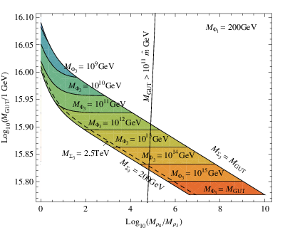
where the upper bound is coming from the unification and proton decay constraints [7] and the lower bound is due to the minimal allowed value for $M_{\rho_{3}}$. We recall that $\hat{m}$ is the mass splitting. From Eq. (43) one readily obtains an upper bound on the mass splitting between the fields in the adjoint representation:

where the lower bound comes from the unification constraints [7]. Therefore, one excludes a large part of the allowed parameter space shown in reference [7]. In order to show the importance of these bounds we present in Fig. 3 the parameter space allowed by unification when $M_{\Phi_{1}}=200$ GeV. The fields $\Phi_{1}\sim(8,2,1/2)$ and $\Phi_{3}\sim(3,3,-1/3)$ live in ${\bf 45_{H}}$ while $\Sigma_{3}\sim(1,3,0)$ is in ${\bf 24_{H}}$. See reference [7] for details. Notice that once we include the leptogenesis constraints a large part of the parameter space is excluded. Now, since $M_{\Phi_{3}}$ has to be larger than $10^{12}$ GeV in order to satisfy the constraints coming from proton decay, the only allowed region in Fig. 3 is the area bounded by the lines $M_{\Sigma_{3}}=200$ GeV, $M_{\Phi_{3}}=10^{12}$ GeV and $M_{\rm GUT}=10^{11}\hat{m}$ GeV. This means that the model is quite predictive.

We have presented a detailed study of the Baryogenesis via Leptogenesis mechanism in the context of Adjoint $SU(5)$ where neutrino masses are generated by the Type I and Type III seesaw mechanisms. Through the decays of the field responsible for the Type III seesaw, $\rho_{3}$, a lepton asymmetry is produced and later converted in a baryon asymmetry by sphalerons. In our model, the $C\!P$ asymmetry is generated by the vertex correction since the self-energy contribution vanishes. Imposing successful leptogenesis, we found that the case of normal hierarchy for the neutrinos is possible for a large range of $\rho_{3}$ masses (see Fig. 1). On the other hand, when the spectrum is inverted, the allowed region is very small (see Fig. 2). Finally, we have shown that, imposing successful leptogenesis, one rules out a large region in the parameter space allowed by the unification of gauge interactions and the constraints coming from proton decay (see Fig. 3).