From subfactor planar algebras to subfactors

This paper contains no new results. What it does is to give a different proof of the main result of [GnnJnsShl] which, in turn, offers an alternative proof of an important result of Popa in [Ppa] that may be paraphrased as saying that any subfactor planar algebra arises from an extremal subfactor.

In this introductory section, we will briefly review the main result of [GnnJnsShl] and the ingredients of its proof and compare and contrast the proof presented here with that one.

The main result of [GnnJnsShl] begins with the construction of a tower $Gr_{k}(P)$ of graded $*$-algebras with compatible traces $Tr_{k}$ associated to a subfactor planar algebra $P$. Next, appealing to a result in [PpaShl], the planar algebra $P$ is considered as embedded as a planar subalgebra of the planar algebra of a bipartite graph as described in [Jns2]. It is shown that that the traces $Tr_{k}$ are faithful and positive and then $II_{1}$-factors $M_{k}$ are obtained by appropriate completions (in case the modulus $\delta>1$ - which is the only real case of interest). It is finally seen that the tower of $M_{k}$’s is the basic construction tower for (the finite index, extremal $II_{1}$-subfactor) $M_{0}\subseteq M_{1}$ and that the planar algebra of this subfactor is naturally isomorphic to the original planar algebra $P$. The proofs all rely on techniques of free probability and random matrices and indeed, one of the stated goals of the paper is to demonstrate the connections between these and planar algebras.

The raison d’être of this paper is to demonstrate the power of planar algebra techniques. We begin with a short summary of our notations and conventions regarding planar algebras in Section 2. In Section 3, we describe a tower $F_{k}(P)$ of filtered $*$-algebras, with compatible traces and ‘conditional expectations’, associated to a subfactor planar algebra $P$. The positivity of the traces being obvious, we show in Section 4 that the associated GNS representations are bounded and thus yield a tower of finite von Neumann algebra completions. The heart of this paper is Section 5 which is devoted to showing that these completions are factors and to computations of some relative commutants. The penultimate Section 6 identifies the tower as a basic construction tower of a finite index extremal subfactor with associated planar algebra as the original $P$. The final section exhibits interesting trace preserving $*$-isomorphisms between the algebras $Gr_{k}(P)$ of [GnnJnsShl] and our $F_{k}(P)$, thus justifying - to some extent - the first sentence of this paper.

All our proofs rely solely on planar algebra techniques and in that sense our paper is mostly self-contained. We will need neither the embedding theorem for a subfactor planar algebra into the planar algebra of a bipartite graph nor any free probability or random matrix considerations. In the trade-off between analytic techniques and algebraic/combinatorial techniques that is characteristic of subfactor theory, it would be fair to say that [GnnJnsShl] leans towards the analytic approach while this paper takes the opposite tack.

After this paper had been written, we communicated it to Jones requesting his comments. He wrote back saying that this “may be similar to [JnsShlWlk]” which appears on his homepage; and we discovered that this is indeed the case.

The purpose of this section is to fix our notations and conventions regarding planar algebras. We assume that the reader is familiar with planar algebras as in [Jns] or in [KdySnd] so we will be very brief.

Recall that the basic structure that underlies planar algebras is an action by the ‘coloured operad of planar tangles’ which concept we will now explain. Consider the set $Col=\{0_{+},0_{-},1,2,\cdots\}$, whose elements are called colours.

We will not define a tangle but merely note the following features. Each tangle has an external box, denoted $D_{0}$, and a (possibly empty) ordered collection of internal non-nested boxes denoted $D_{1}$, $D_{2}$, $\cdots$. Each box has an even number (again possibly 0) of points marked on its boundary. A box with $2n$ points on its boundary is called an $n$-box or said to be of colour $n$. There is also given a collection of disjoint curves each of which is either closed, or joins a marked point on one of the boxes to another such. For each box having at least one marked point on its boundary, one of the regions ( = connected components of the complement of the boxes and curves) that impinge on its boundary is distinguished and marked with a $*$ placed near its boundary. The whole picture is to be planar and each marked point on a box must be the end-point of one of the curves. Finally, there is given a chequerboard shading of the regions such that

the $*$-region of any box is shaded white. A $0$-box is said to be $0_{+}$ box if the region touching its boundary is white and a $0_{-}$ box otherwise. A $0$ without the $\pm$ qualification will always refer to $0_{+}$. A tangle is said to be an $n$-tangle if its external box is of colour $n$. Tangles are defined only upto a planar isotopy preserving the $*$’s, the shading and the ordering of the internal boxes.

We illustrate several important tangles in Figure 1.

This figure (along with others in this paper) uses the following notational device for convenience in drawing tangles. A strand in a tangle with a non-negative integer, say $t$, adjacent to it will indicate a $t$-cable of that strand, i.e., a parallel cable of $t$ strands, in place of the one actually drawn. Thus for instance, the tangle equations of Figure 2 hold.

In the sequel, we will have various integers adjacent to strands in tangles and leave it to the reader to verify in each case that the labelling integers are indeed non-negative.

A useful labelling convention for tangles (that we will not be very consistent in using though) is to decorate its tangle symbol, such as $I,EL,M$ or $TR$, with subscripts and a superscript that give the colours of its internal boxes and external box respectively. With this, we may dispense with showing the shading, which is then unambiguously determined. Another useful device is to label the marked points on any $n$-box with the numbers $1,2,\cdots,2n-1,2n$ in a clockwise fashion so that the interval from $2n$ to $1$ is in its $*$-region.

The basic operation that one can perform on tangles is substitution of one into a box of another. If $T$ is a tangle that has some internal boxes $D_{i_{1}},\cdots,D_{i_{j}}$ of colours $n_{i_{1}},\cdots,n_{i_{j}}$ and if $S_{1},\cdots,S_{j}$ are arbitrary tangles of colours $n_{i_{1}},\cdots,n_{i_{j}}$, then we may substitute $S_{t}$ into the box $D_{i_{t}}$ of $T$ for each $t$ - such that the ‘$*$’s match’ - to get a new tangle that will be denoted $T\circ_{(D_{i_{1}},\cdots,D_{i_{j}})}(S_{1},\cdots,S_{j})$. The collection of tangles along with the substitution operation is called the coloured operad of planar tangles.

A planar algebra $P$ is an algebra over the coloured operad of planar tangles. By this, is meant the following: $P$ is a collection $\{P_{n}\}_{n\in Col}$ of vector spaces and linear maps $Z_{T}:P_{n_{1}}\otimes P_{n_{2}}\otimes\cdots\otimes P_{n_{b}}\rightarrow P_{n_{0}}$ for each $n_{0}$-tangle $T$ with internal boxes of colours $n_{1},n_{2},\cdots,n_{b}$. The collection of maps is to be ‘compatible with substitution of tangles and renumbering of internal boxes’ in an obvious manner. For a planar algebra $P$, each $P_{n}$ acquires the structure of an associative, unital algebra with multiplication defined using the tangle $M_{n,n}^{n}$ and unit defined to be $1_{n}=Z_{1^{n}}(1)$.

Among planar algebras, the ones that we will be interested in are the subfactor planar algebras. These are complex, finite-dimensional and connected in the sense that each $P_{n}$ is a finite-dimensional complex vector space and $P_{0_{\pm}}$ are one dimensional. They have a positive modulus $\delta$, meaning that closed loops in a tangle $T$ contribute a multiplicative factor of $\delta$ in $Z_{T}$. They are spherical in that for a $0$-tangle $T$, the function $Z_{T}$ is not just planar isotopy invariant but also an isotopy invariant of the tangle regarded as embedded on the surface of the two sphere. Further, each $P_{n}$ is a $C^{*}$-algebra in such a way that for an $n_{0}$-tangle $T$ with internal boxes of colours $n_{1},n_{2},\cdots,n_{b}$ and for $x_{i}\in P_{n_{i}}$, the equality $Z_{T}(x_{1}\otimes\cdots\otimes x_{b})^{*}~=~Z_{T^{*}}(x_{1}^{*}\otimes\cdots\otimes x_{b}^{*})$ holds, where $T^{*}$ is the adjoint of the tangle $T$ - which, by definition, is obtained from $T$ by reflecting it.

Finally, the trace $\tau:P_{n}\rightarrow{\mathbb{C}}=P_{0}$ defined by:

is postulated to be a faithful, positive (normalised) trace for each $n\geq 0$.

We then have the following fundamental thorem of Jones in [Jns].

Recall that a finite index $II_{1}$-subfactor $N\subseteq M$ is said to be extremal if the restriction of the traces on $N^{\prime}$ (computed in ${\mathcal{L}}(L^{2}(M))$) and $M$ to $N^{\prime}\cap M$ agree. The notations $E_{M^{\prime}\cap M_{n+1}}$ and $E_{N^{\prime}\cap M_{n}}$ stand for the trace preserving conditional expectations of $N^{\prime}\cap M_{n+1}$ onto $M^{\prime}\cap M_{n+1}$ and $N^{\prime}\cap M_{n}$ respectively.

The converse part of Jones’ theorem is, in essence, the result of Popa alluded to in the introduction, as remarked in [Jns]. It is this converse, as proved in [GnnJnsShl], for which we supply a different proof in the rest of this paper.

We note that the multiplication tangle here agrees with the one in [GnnJnsShl] but is adjoint to the ones in [Jns] and in [KdySnd] while the rotation tangle is as in [KdySnd] but adjoint to the one in [Jns].

For the rest of this paper, the following notation will hold. Let $P$ be a subfactor planar algebra of modulus $\delta>1$. We therefore have finite-dimensional $C^{*}$-algebras $P_{n}$ for $n\in Col$ with appropriate inclusions. For $x\in P_{n}$, set $||x||_{P_{n}}=\tau(x^{*}x)^{\frac{1}{2}}$; this defines a norm on $P_{n}$.

For $k\geq 0$, let $F_{k}(P)$ be the vector space direct sum $\oplus_{n=k}^{\infty}P_{n}$ (where $0=0_{+}$, here and in the sequel). Our goal, in this section, is to equip each $F_{k}(P)$ with a filtered, associative, unital $*$-algebra structure with normalised trace $t_{k}$ and to describe trace preserving filtered $*$-algebra inclusions $F_{0}(P)\subseteq F_{1}(P)\subseteq F_{2}(P)\subseteq\cdots$, as well as conditional expectation-like maps $F_{0}(P)\stackrel{{\scriptstyle E_{0}}}{{\leftarrow}}F_{1}(P)\stackrel{{\scriptstyle E_{1}}}{{\leftarrow}}F_{2}(P)\stackrel{{\scriptstyle E_{2}}}{{\leftarrow}}\cdots$.

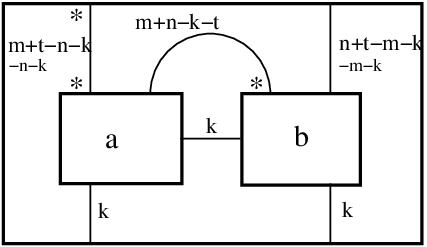
We begin by defining the multiplication. For $a\in F_{k}(P)$, we will denote by $a_{n}$, its $P_{n}$ component for $n\geq k$. Thus $a=\sum_{n=k}^{\infty}a_{n}=(a_{k},a_{k+1},\cdots)\in F_{k}(P)$, where only finitely many $a_{n}$ are non-zero. Now suppose that $a=a_{m}\in P_{m}$ and $b=b_{n}\in P_{n}$ where $m,n\geq k$. Their product in $F_{k}(P)$, denoted¹¹ 1 Rather than being notationally correct and write $\#_{k}$, we drop the subscript in the interests of aesthetics. $a\#b$, is defined to be $\sum_{t=|n-m|+k}^{n+m-k}(a\#b)_{t}$ where $(a\#b)_{t}$ is given by the tangle in Figure 3.

Define $\#$ by extending this map bilinearly to the whole of $F_{k}(P)\times F_{k}(P)$.

As in [GnnJnsShl], we will reserve ‘$*$’ to denote the usual involution on $P_{n}$’s and use $\dagger$ (rather than $\dagger_{k}$) to denote the involution on $F_{k}(P)$. For $a=a_{m}\in P_{m}\subseteq F_{k}(P)$ define $a^{\dagger}\in P_{m}$ by the tangle in Figure 4

and extend additively to the whole of $F_{k}(P)$. Note that $a^{\dagger}=Z_{(R^{m}_{m})^{k}}(a^{*})$ where $R_{m}^{m}$ is the $m$-rotation tangle and $(R^{m}_{m})^{k}=R_{m}^{m}\circ R_{m}^{m}\circ\cdots\circ R_{m}^{m}$ ($k$ factors).

Next, define the linear functional $t_{k}$ on $F_{k}(P)$ to be the normalised trace of its $P_{k}$ component, i.e., for $a=(a_{k},a_{k+1},\cdots)\in F_{k}(P)$ define $t_{k}(a)=\tau(a_{k})$.

Then, define the ‘inclusion map’ of $F_{k-1}(P)$ into $F_{k}(P)$ (for $k\geq 1$) as the map whose restriction takes $P_{n-1}\subseteq F_{k-1}(P)$ to $P_{n}\subseteq F_{k}(P)$ by the tangle illustrated in Figure 5.

Finally, define the conditional expectation-like map $E_{k-1}:F_{k}(P)\rightarrow F_{k-1}(P)$ (for $k\geq 1$) as $\delta^{-1}$ times the map whose restriction takes $P_{n}\subseteq F_{k}(P)$ to $P_{n-1}\subseteq F_{k-1}(P)$ by the tangle illustrated in Figure 6.

An important observation that we use later is that ‘restricted’ to $P_{k}\subseteq F_{k}(P)$, all these maps are the ‘usual’ ones of the planar algebra $P$. More precisely we have (a) $\#|_{P_{k}\otimes P_{k}}=Z_{M^{k}_{k,k}}$, (b) $\dagger|_{P_{k}}=*$, (c) $t_{k}|_{P_{k}}=\tau$, (d) The inclusion of $F_{k-1}(P)$ into $F_{k}(P)$ restricts to $Z_{I_{k-1}^{k}}:P_{k-1}\rightarrow P_{k}$, and (e) $\delta E_{k-1}|_{P_{k}}=Z_{ER^{k-1}_{k}}$.

We can now state the main result of this section.

We define $H_{k}$ to be the Hilbert space completion of $F_{k}(P)$. Note that for the inner-product on $F_{k}(P)$, the subspaces $P_{n}$ of $H_{k}$ are mutually orthogonal and so $H_{k}$ is their orthogonal direct sum $\oplus_{n=k}^{\infty}P_{n}$. In particular, elements of $H_{k}$ are sequences $\xi=(x_{k},x_{k+1},\cdots)$ where $||\xi||_{H_{k}}^{2}=\delta^{-k}\sum_{n=k}^{\infty}\delta^{n}\tau(x_{n}^{*}x_{n})<\infty$.

Our goal in this section is to show that for each $k\geq 0$, the left and right regular representations of $F_{k}(P)$ are both bounded for the norm on $F_{k}(P)$ and therefore extend uniquely to $*$-homomorphisms $\lambda_{k},\rho_{k}:F_{k}(P)\rightarrow{\mathcal{L}}(H_{k})$. We then show that the von Neumann algebras generated by $\lambda_{k}(F_{k}(P))$ and $\rho_{k}(F_{k}(P))$ are finite and commutants of each other. Finally we show that for $k\geq 0$, the finite von Neumann algebras $\lambda_{k}(F_{k}(P))^{\prime\prime}$ naturally form a tower.

The key estimate we need for proving boundedness is contained in Proposition 4.2, the proof of which appeals to the following lemma.

We are ready to prove boundedness of the left regular representation. During the course of the proof we will need to use the fact that $||\sum_{i=1}^{k}a_{i}||^{2}\leq k(\sum_{i=1}^{k}||a_{i}||^{2})$ for vectors $a_{1},\cdots,a_{k}$ in an inner-product space, which follows on applying Cauchy-Schwarz to the vectors $(||a_{1}||,\cdots,||a_{k}||)$ and $(1,1,\cdots,1)$ in ${\mathbb{C}}^{k}$.

It follows from Proposition 4.3 that for any $a\in F_{k}(P)$, the map $\lambda_{k}(a)$ is bounded and thus extends uniquely to an element of ${\mathcal{L}}(H_{k})$. We then get a $*$-representation $\lambda_{k}:F_{k}(P)\rightarrow{\mathcal{L}}(H_{k})$.

In order to avoid repeating hypotheses we make the following definition. By a finite pre-von Neumann algebra, we will mean a complex $*$-algebra $A$ that is equipped with a normalised trace $t$ such that (i) the sesquilinear form defined by $\langle a^{\prime}|a\rangle=t(a^{*}a^{\prime})$ defines an inner-product on $A$ and such that (ii) for each $a\in A$, the left-multiplication map $\lambda_{A}(a):A\rightarrow A$ is bounded for the trace induced norm of $A$. Examples that we will be interested in are the $F_{k}(P)$ with their natural traces $t_{k}$ for $k\geq 0$. We then have the following simple lemma which motivates the terminology and whose proof we sketch in some detail.