Testing the Nullspace Property
using Semidefinite Programming
Abstract
Recent results in compressed sensing show that, under certain conditions, the sparsest solution to an underdetermined set of linear equations can be recovered by solving a linear program. These results either rely on computing sparse eigenvalues of the design matrix or on properties of its nullspace. So far, no tractable algorithm is known to test these conditions and most current results rely on asymptotic properties of random matrices. Given a matrix , we use semidefinite relaxation techniques to test the nullspace property on and show on some numerical examples that these relaxation bounds can prove perfect recovery of sparse solutions with relatively high cardinality.
Keywords: Compressed sensing, nullspace property, semidefinite programming, restricted isometry constant.
1 Introduction
A recent stream of results in signal processing have focused on producing explicit conditions under which the sparsest solution to an underdetermined linear system can be found by solving a linear program. Given a matrix with and a vector , writing the number of nonzero coefficients in , this means that the solution of the following (combinatorial) minimization problem:
| (1) |
in the variable , can be found by solving the (convex) minimization problem:
| (2) |
in the variable , which is equivalent to a linear program.
Based on results by Vershik and Sporyshev (1992) and Affentranger and Schneider (1992), Donoho and Tanner (2005) show that when the solution of (1) is sparse with and the coefficients of are i.i.d. Gaussian, then the solution of the problem in (2) will always match that of the problem in (1) provided is below an explicitly computable strong recovery threshold . They also show that if is below another (larger) weak recovery threshold , then these solutions match with an exponentially small probability of failure.
Universal conditions for strong recovery based on sparse extremal eigenvalues were derived in Candès and Tao (2005) and Candès and Tao (2006) who also proved that certain (mostly random) matrix classes satisfied these conditions with an exponentially small probability of failure. Simpler, weaker conditions which can be traced back to Donoho and Huo (2001), Zhang (2005) or Cohen et al. (2009) for example, are based on properties of the nullspace of . In particular, if we define
these references show that guarantees strong recovery.
One key issue with the current sparse recovery conditions in Candès and Tao (2005) or Donoho and Huo (2001) is that except for explicit recovery thresholds available for certain types of random matrices, testing these conditions on generic matrices is potentially harder than solving the combinatorial -norm minimization problem in (1) for example as it implies either solving a combinatorial problem to compute , or computing sparse eigenvalues. Semidefinite relaxation bounds on sparse eigenvalues were used in d’Aspremont et al. (2008) or Lee and Bresler (2008) for example to test the restricted isometry conditions in Candès and Tao (2005) on arbitrary matrices. In recent independent results, Juditsky and Nemirovski (2008) provide an alternative proof of some of the results in Donoho and Huo (2001), extend them to the noisy case and produce a linear programming (LP) relaxation bound on with explicit performance bounds.
In this paper, we derive a semidefinite relaxation bound on , study its tightness and performance. By randomization, the semidefinite relaxation also produces lower bounds on the objective value as a natural by-product of the solution. Overall, our bounds are slightly better than LP ones numerically but both relaxations share the same asymptotic performance limits. However, because it involves solving a semidefinite program, the complexity of the semidefinite relaxation derived here is significantly higher than that of the LP relaxation.
The paper is organized as follows. In Section 2, we briefly recall some key results in Donoho and Huo (2001) and Cohen et al. (2009). We derive a semidefinite relaxation bound on in Section 3, and study its tightness and performance in Section 4. Section 5 describes a first-order algorithm to solve the resulting semidefinite program. Finally, we test the numerical performance of this relaxation in Section 6.
Notation
To simplify notation here, for a matrix , we write its columns , the sum of absolute values of its coefficients (not the norm of its spectrum) and the largest coefficient magnitude. More classically, and are the Frobenius and spectral norms.
2 Sparse recovery & the null space property
Given a coding matrix with , a sparse signal and an information vector such that
we focus on the problem of perfectly recovering the signal from the vector , assuming the signal is sparse enough. We define the decoder as a mapping from , with
| (3) |
This particular decoder is equivalent to a linear program which can be solved efficiently. Suppose that the original signal is sparse, a natural question to ask is then: When does this decoder perfectly recover a sparse signal ? Recent results by Candès and Tao (2005), Donoho and Tanner (2005) and Cohen et al. (2009) provide a somewhat tight answer. In particular, as in Cohen et al. (2009), for a given coding matrix and , we can quantify the error of a decoder by computing the smallest constant such that
| (4) |
for all , where
is the error of the best -term approximation of the signal and can simply be computed as the norm of the smallest coefficients of . We now define the nullspace property as in Donoho and Huo (2001) or Cohen et al. (2009).
Definition 1
A matrix satisfies the null space property in of order with constant if and only if
| (5) |
holds for all with and index subsets of cardinality , where is the complement of in .
Cohen et al. (2009) for example show the following theorem linking the optimal decoding quality on sparse signals and the nullspace property constant .
Theorem 2
Proof. See (Cohen et al., 2009, Corollary 3.3).
This last result means that the existence of an optimal decoder staisfying (4) is equivalent to satisfying (5). Unfortunately, this optimal decoder is defined as
hence requires solving a combinatorial problem which is potentially intractable. However, using tighter restrictions on the nullspace property constant , we get the following result about the linear programming decoder in (3).
Theorem 3
Proof. See steps (4.3) to (4.10) in the proof of (Cohen et al., 2009, Theorem 4.3).
To summarize the results above, if there exists a such that the coding matrix satisfies the nullspace property in (5) at the order then there exists a decoder which perfectly recovers signals with cardinality . If, in addition, we can show that , then the linear programming based decoder in (3) perfectly recovers signals with cardinality . In the next section, we produce upper bounds on the constant in (5) using semidefinite relaxation techniques.
3 Semidefinite Relaxation
Given and , we look for a constant in (5) such that
for all vectors with and index subsets with cardinality . We can rewrite this inequality
| (6) |
with . Because , if we can show that then we prove that satisfies the nullspace property at order with constant . Furthermore, if we prove , we prove the existence of a linear programming based decoder which perfectly recovers signals with at most errors. By homogeneity, the constant can be computed as
| (7) |
where the equality can, without loss of generality, be replaced by . We now derive a semidefinite relaxation for problem (7) as follows. After a change of variables
we can rewrite (7) as
| (8) |
in the variables , , where all norms should be understood componentwise. We then simply drop the rank constraint to form a relaxation of (7) as
| (9) |
which is a semidefinite program in the variables , . Note that the contraint is redundant in the rank one problem but not in its relaxation. Because all constraints are linear here, dropping the rank constraint is equivalent to computing a Lagrangian (bidual) relaxation of the original problem and adding redundant constraints to the original problem often tightens these relaxations. The dual of program (9) can be written
which is a semidefinite program in the variables and . For any feasible point of this program, the objective is an upper bound on the optimal value of (9), hence on . We can further simplify this program using elimination results for LMIs. In fact, (Boyd et al., 1994, §2.6.2) shows that this last problem is equivalent to
| (10) |
where the variable is now scalar. In fact, using the same argument, letting be an orthogonal basis of the nullspace of , i.e. such that with , we can rewrite the previous problem as follows
| (11) |
which is a (smaller) semidefinite program in the variables and . The dual of this last problem is then
| (12) |
which is a semidefinite program in the matrix variables , whose objective value is equal to that of problem (9).
Note that adding any number of redundant constraints in the original problem (8) will further improve tightness of the semidefinite relaxation, at the cost of increased complexity. In particular, we can use the fact that when
and if we set and , we must have
and
for . This means that we can refine the constraint in (9) to solve instead
| (13) |
which is a semidefinite program in the variables , and . Adding these columnwise constraints on and significantly tightens the relaxation. Any feasible solution to the dual of (13) with objective value less than will then be a certificate that .
4 Tightness & Limits of Performance
The relaxation above naturally produces a covariance matrix as its output and we use randomization techniques as in Goemans and Williamson (1995) to produce primal solutions for problem (7). Then, following results by A. Nemirovski (private communication), we bound the performance of the relaxation in (9).
4.1 Randomization
Here, we show that lower bounds on can be generated as a natural by-product of the relaxation. We use solutions to the semidefinite program in (9) and generate feasible points to (7) by randomization. These can then be used to certify that and prove that a matrix does not satisfy the nullspace property. Suppose that the matrix
| (14) |
solves problem (9), because , we can generate Gaussian variables . Below, we show that after proper scaling, will satisfy the constraints of problem (7) with high probability, and use this result to quantify the quality of these randomized solutions. We begin by recalling classical results on the moments of and when and bound deviations above their means using concentration inequalities on Lipschitz functions of Gaussian variables.
Lemma 1
Let , and , we have
| (15) |
Proof. Let be the square root of and be independent Gaussian variables, we have
hence, because each term is a Lipschitz continuous function of the variables with constant , is Lipschitz with constant . Using the concentration inequality by Ibragimov et al. (1976) (see also Massart (2007) for a general discussion) we get for any
with . Picking and yields the desired result.
We now recall another classic result on the concentration of , also based on the fact that is a Lipschitz continuous function of independent Gaussian variables.
Lemma 2
Let , and then
| (16) |
Proof. (Massart, 2007, Theorem 3.12) shows that is a Lipschitz function of independent Gaussian random variables with constant , hence a reasoning similar to that in lemma 1 yields the desired result.
Using union bounds, the lemmas above show that if we pick and , the scaled sample points
will be feasible in (7) with probability at least if we set
| (17) |
and
| (18) |
The randomization technique is then guaranteed to produce a feasible point of (7) with objective value
where is the quantile of when . We now compute a (relatively coarse) lower bound on the value of that quantile.
Lemma 3
Proof. Let be such that and , we have
where is a standard normal vector of dimension . Wick’s formula implies
where is the Hafnian of the matrix (see Barvinok (2007) for example), which means
Because , we then conclude using Cantelli’s inequality, which gives
having set .
We can now combine these results to produce a lower bound on the objective value achieved by randomization.
Theorem 4
Proof. If solves (9) and the vectors are sampled according to , then
means that we always have . When , Lemmas 1 and 2 show that
will be feasible in (7) with probability at least , hence we can get a feasible point for (7) by sampling enough variables . Lemma 3 shows that if we set as above, the randomization procedure is guaranteed to reach an objective value at least equal to
which is the desired result.
Note that because , we have , hence . We also have hence
and the only a priori unknown terms controlling tightness are , and . Unfortunately, while the third term is bounded by one, the first two can become quite large, with trivial bounds giving
which means that, in the worst case, our lower bound will be off by a factor . However, we will observe in Section 6 that, when , these terms are sometimes much lower than what the worst-case bounds seem to indicate. The expression for the tightness coefficient in (14) also highlights the importance of the constraint . Indeed, the positive semidefinitess of principal submatrices means that , hence
so controlling potentially tightens the relaxation. This is confirmed in numerical experiments: the relaxation including the (initially) redundant norm constraint on is significantly tighter on most examples. Finally, note that better lower bounds on can be obtained (numerically) by sampling in (6) directly, or as suggested by one of the referees, solving
in for various random vectors with at most nonzero coefficients. In both cases unfortunately, the moments cannot be computed explicitly so studying performance is much harder.
4.2 Performance
Following results by A. Nemirovski (private communication), we can derive precise bounds on the performance of the relaxation in (9).
Lemma 4
Proof. First, notice that when the matrices solve (9), with
means that the rows of also belong to the nullspace of . If satisfies the nullspace property in (6), we must have for hence . By construction, we always have hence when solves (9) with .
As in Juditsky and Nemirovski (2008), this also means that if a matrix satisfies the restricted isometry property at cardinality (as Gaussian matrices do for example), then the relaxation in (9) will certify for . Unfortunately, the results that follow show that this is the best we can hope for here.
Without loss of generality, we can assume that (if , the problem is harder). Let be an orthoprojector on a -dimensional subspace of the nullspace of , with . By construction, , and of course . We can use this matrix to construct a feasible solution to problem (13) when . We set , , , and for . We then have
and with . We also get
With
the matrices we have defined above form a feasible point of problem (13). Because, , this feasible point proves that the optimal value of (13) is larger than when and . This means that the relaxation in (13) can prove that a matrix satisfies the nullspace property for cardinalities at most and this performance bound is tight since we have shown that it achieves this rate of for good matrices.
This counter example also produces bounds on the performance of another relaxation for testing sparse recovery. In fact, if we set with defined as above, we have with and
and is an optimal solution of the problem
which is a semidefinite relaxation used in d’Aspremont et al. (2007) and d’Aspremont et al. (2008) to bound the restricted isometry constant . Because by construction, we know that this last relaxation will fail to show whenever . Somewhat strikingly, this means that the three different tractable tests for sparse recovery conditions, derived in d’Aspremont et al. (2008), Juditsky and Nemirovski (2008) and this paper, are all limited to showing recovery at the (suboptimal) rate .
5 Algorithms
Small instances of the semidefinite program in (11) and be solved efficiently using solvers such as SEDUMI (Sturm, 1999) or SDPT3 (Toh et al., 1999). For larger instances, it is more advantageous to solve (11) using first order techniques, given a fixed target for . We set to be an orthogonal basis of the nullspace of the matrix in (6), i.e. such that with . We also let be a target critical value for (such as for example), and solve the following problem
| (22) |
in the variables and . If the objective value of this last problem is greater than zero, then the optimal value of problem (11) is necessarily smaller than , hence in (7).
Because this problem is a minimum eigenvalue maximization problem over a simple compact (a norm ball in fact), large-scale instances can be solved efficiently using projected gradient algorithms or smooth semidefinite optimization techniques (Nesterov, 2007; d’Aspremont et al., 2007). As we show below, the complexity of projecting on this ball is quite low.
Lemma 5
The complexity of projecting on
is bounded by , where is the target precision in projecting.
Proof. By duality, solving
in the variables is equivalent to solving
in the variable . For a fixed , we can get the derivative w.r.t. by solving four separate penalized least-squares problems. Each of these problems can be solved explicitly in at most (by shrinking the current point) so the complexity of solving the outer maximization problem up to a precision by binary search is
We can then implement the smooth minimization algorithm detailed in (Nesterov, 2005, §5.3) to a smooth approximation of problem (22) as in Nesterov (2007) or d’Aspremont et al. (2007) for example. Let be a regularization parameter. The function
| (23) |
satifies
for any . Furthermore, is a smooth approximation of the function , and is Lipschitz continuous with constant . Let be a given target precision, this means that if we set then
| (24) |
will be an approximation of the objective function in (22). Whenever , we must have
hence, following (Nesterov, 2007, §4), the gradient of is Lipschitz continuous with respect to the Frobenius norm, with Lipschitz constant given by
We then define the compact, convex set as
and define a prox function over as , which is strongly convex with constant w.r.t. the Frobenius norm. Starting from , the algorithm in Nesterov (2005) for solving
where is defined in (24), proceeds as follows.
Repeat:
- 1.
Compute and
- 2.
Find
- 3.
Find
- 4.
Set
Until gap .
Step one above computes the (smooth) function value and gradient. The second step computes the gradient mapping, which matches the gradient step for unconstrained problems (see (Nesterov, 2003, p.86)). Step three and four update an estimate sequence see (Nesterov, 2003, p.72) of whose minimum can be computed explicitly and gives an increasingly tight upper bound on the minimum of . We now present these steps in detail for our problem.
Step 1
The most expensive step in the algorithm is the first, the computation of and its gradient. This amounts to computing the matrix exponential in (23) at a cost of (see Moler and Van Loan (2003) for details).
Step 2
This step involves solving a problem of the form
where is given. The above problem can be reduced to an Euclidean projection on
| (25) |
where is given. According to Lemma 5, this can be solved opearations.
Step 3
The third step involves solving an Euclidean projection problem similar to (25), with defined here by:
Stopping criterion
We stop the algorithm when the duality gap is smaller than the target precision . The dual of the binary optimization problem (22) can be written
| (26) |
in the block matrix variable with blocks , . Since the gradient produces a dual feasible point by construction, we can use it to compute a dual objective value and bound the duality gap at the current point .
Complexity
According to Nesterov (2007), the total worst-case complexity to solve (22) with absolute accuracy less than is then given by
Each iteration of the algorithm requires computing a matrix exponential at a cost of and the algorithm requires iterations to reach a target precision of . Note that while this smooth optimization method can be used to produce reasonable complexity bounds for checking if the optimal value of (22) is positive, i.e. if , in practice the algorithm is relatively slow and we mostly use interior point solvers on smaller problems to conduct experiments in the next section.
6 Numerical Results
In this section, we illustrate the numerical performance of the semidefinite relaxation detailed in section 3.
6.1 Illustration
We test the semidefinite relaxation in (11) on a sample of ten random Gaussian matrices with , and . For each of these matrices, we solve problem (11) for to produce upper bounds on , hence on in (5), with . From Donoho and Huo (2001), we know that if then we can bound the decoding error in (4), and if then the original signal can be recovered exactly by solving a linear program. We also plot the randomized values for with together with the semidefinite relaxation bound.
 |
 |
 |
 |
Next, in Figure 2, we use a Gaussian matrix with , and and, for each , we sample fifty information vectors where is uniformly distributed and has cardinality . On the left, we plot the probability of recovering the original sparse signal using the linear programming decoder in (3). On the right, we plot the mean recovery error using the linear programming decoder in (3) and compare it with the bound induced by Theorem 3.
6.2 Performance on compressed sensing matrices
In tables 1, 2 and 3, we compare the performance of the linear programming relaxation bound on derived in Juditsky and Nemirovski (2008) with that of the semidefinite programming bound detailed in Section 3. We test these bounds for various matrix shape ratios , target cardinalities on matrices with Fourier, Bernoulli or Gaussian coefficients using SDPT3 by Toh et al. (1999) to solve problem (11). We show median bounds computed over ten sample matrices for each type, hence test a total of 600 different matrices. We compare these relaxation bounds with the upper bounds produced by sequential convex optimization as in Juditsky and Nemirovski (2008, §4.1). In the Gaussian case, we also compare these relaxation bounds with the asymptotic thresholds on strong and weak (high probability) recovery discussed in Donoho and Tanner (2008). The semidefinite bounds on always match with the LP bounds in Juditsky and Nemirovski (2008) when (both are tight), and are often smaller than LP bounds whenever is greater than 1 on Gaussian or Bernoulli matrices. The semidefinite upper bound on was smaller than the LP one in 563 out of the 600 matrices sampled here, with the difference ranging from 4e-2 to -9e-4. Of course, this semidefinite relaxation is significantly more expensive than the LP based one and that these experiments thus had to be performed on very small matrices.
| Relaxation | Upper bound | ||||||
|---|---|---|---|---|---|---|---|
| LP | 0.5 | 0.21 | 0.38 | 0.57 | 0.82 | 0.98 | 2 |
| SDP | 0.5 | 0.21 | 0.38 | 0.57 | 0.82 | 0.98 | 2 |
| SDP low. | 0.5 | 0.05 | 0.10 | 0.16 | 0.24 | 0.32 | 2 |
| LP | 0.6 | 0.16 | 0.31 | 0.46 | 0.61 | 0.82 | 3 |
| SDP | 0.6 | 0.16 | 0.31 | 0.46 | 0.61 | 0.82 | 3 |
| SDP low. | 0.6 | 0.04 | 0.09 | 0.15 | 0.20 | 0.31 | 3 |
| LP | 0.7 | 0.12 | 0.25 | 0.39 | 0.50 | 0.62 | 4 |
| SDP | 0.7 | 0.12 | 0.25 | 0.39 | 0.50 | 0.62 | 4 |
| SDP low. | 0.7 | 0.04 | 0.09 | 0.14 | 0.18 | 0.22 | 4 |
| LP | 0.8 | 0.10 | 0.20 | 0.30 | 0.38 | 0.48 | 6 |
| SDP | 0.8 | 0.10 | 0.20 | 0.30 | 0.38 | 0.48 | 6 |
| SDP low. | 0.8 | 0.04 | 0.07 | 0.13 | 0.17 | 0.23 | 6 |
| Relaxation | Strong | Weak | ||||||
|---|---|---|---|---|---|---|---|---|
| LP | 0.5 | 0.27 | 0.49 | 0.67 | 0.83 | 0.97 | 2 | 11 |
| SDP | 0.5 | 0.27 | 0.49 | 0.65 | 0.81 | 0.94 | 2 | 11 |
| SDP low. | 0.5 | 0.27 | 0.31 | 0.33 | 0.32 | 0.35 | 2 | 11 |
| LP | 0.6 | 0.22 | 0.41 | 0.57 | 0.72 | 0.84 | 2 | 12 |
| SDP | 0.6 | 0.22 | 0.41 | 0.56 | 0.70 | 0.82 | 2 | 12 |
| SDP low. | 0.6 | 0.22 | 0.29 | 0.31 | 0.32 | 0.36 | 2 | 12 |
| LP | 0.7 | 0.20 | 0.34 | 0.47 | 0.60 | 0.71 | 3 | 14 |
| SDP | 0.7 | 0.20 | 0.34 | 0.46 | 0.59 | 0.70 | 3 | 14 |
| SDP low. | 0.7 | 0.20 | 0.27 | 0.31 | 0.35 | 0.38 | 3 | 14 |
| LP | 0.8 | 0.15 | 0.26 | 0.37 | 0.48 | 0.58 | 3 | 16 |
| SDP | 0.8 | 0.15 | 0.26 | 0.37 | 0.48 | 0.58 | 3 | 16 |
| SDP low. | 0.8 | 0.15 | 0.23 | 0.28 | 0.33 | 0.38 | 3 | 16 |
| Relaxation | Upper bound | ||||||
|---|---|---|---|---|---|---|---|
| LP | 0.5 | 0.25 | 0.45 | 0.64 | 0.82 | 0.97 | 2 |
| SDP | 0.5 | 0.25 | 0.45 | 0.63 | 0.80 | 0.94 | 2 |
| SDP low. | 0.5 | 0.25 | 0.28 | 0.29 | 0.29 | 0.34 | 2 |
| LP | 0.6 | 0.21 | 0.38 | 0.55 | 0.69 | 0.83 | 3 |
| SDP | 0.6 | 0.21 | 0.38 | 0.54 | 0.68 | 0.81 | 3 |
| SDP low. | 0.6 | 0.21 | 0.26 | 0.29 | 0.33 | 0.34 | 3 |
| LP | 0.7 | 0.17 | 0.32 | 0.46 | 0.58 | 0.70 | 4 |
| SDP | 0.7 | 0.17 | 0.32 | 0.46 | 0.58 | 0.69 | 4 |
| SDP low. | 0.7 | 0.17 | 0.24 | 0.29 | 0.33 | 0.37 | 4 |
| LP | 0.8 | 0.14 | 0.26 | 0.38 | 0.47 | 0.57 | 5 |
| SDP | 0.8 | 0.14 | 0.26 | 0.37 | 0.47 | 0.57 | 5 |
| SDP low. | 0.8 | 0.14 | 0.21 | 0.27 | 0.33 | 0.38 | 5 |
6.3 Tightness
Section 4 shows that the tightness of the semidefinite relaxation is explicitly controlled by the following quantity
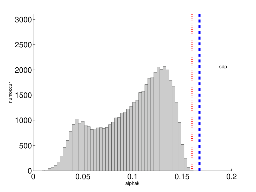
where and are defined in (17) and (18) respectively. In Figure 3, we plot the histogram of values of for all 600 sample matrices computed above, and plot the same histogram on a subset of these results where the target cardinality was set to 1. We observe that while the relaxation performed quite well on most of these examples, the randomization bound on performance often gets very large whenever . This can probably be explained by the fact that we only control the mean in Lemma 3, not the quantile. We also notice that is highly concentrated when on Gaussian and Bernoulli matrices (where the results in Tables 2 and 3 are tight), while the performance is markedly worse for Fourier matrices.
Finally, Tables 2 and 3 show that lower bounds on obtained by randomization for Gaussian are always tight (the solution of the SDP was very close to rank one), while performance on higher values of and Fourier matrices is much worse. On 6 of these experiments however, the SDP randomization lower bound was higher than 1/2, which proved that , hence that the matrix did not satisfy the nullspace property at order 5.


6.4 Numerical complexity
We implemented the algorithm of Section (5) in MATLAB and tested it on random matrices. While the code handles matrices with , it is still considerably slower than similar first-order algorithms applied to sparse PCA problems for example (see d’Aspremont et al. (2007)). A possible explanation for this gap in performance is perhaps that the DSPCA semidefinite relaxation is always tight (in practice at least) hence iterates near the solution tend to be very close to rank one. This is not the case here as the matrix in (9) is very rarely rank one and the number of significant eigenvalues has a direct impact on actual convergence speed. To illustrate this point, Figure 4 shows a Scree plot of the optimal solution to (9) for a small Gaussian matrix (obtained by IP methods with a target precision of ), while Table 4 shows, as a benchmark, total CPU time for proving that on Gaussian matrices, for various values of . We set the accuracy and stop the code whenever positive objective values are reached. Unfortunately, performance for larger values of is typically much worse (which is why we used IP methods to run most experiments in this section) and in many cases, convergence is hard to track as the dual objective values computed using the gradient in (26) produces a relatively coarse gap bounds as illustrated in Figure 4 for a small Gaussian matrix.
| 50 | 100 | 200 | 500 | |
|---|---|---|---|---|
| CPU time | 00 h 01 m | 00 h 10 m | 01 h 38 m | 37 h 22 m |
 |
 |
7 Conclusion & Directions for Further Research
We have detailed a semidefinite relaxation for the problem of testing if a matrix satisfies the nullspace property defined in Donoho and Huo (2001) or Cohen et al. (2009). This relaxation is tight for and matches (numerically) the linear programming relaxation in Juditsky and Nemirovski (2008). It is often slightly tighter (again numerically) for larger values of . We can also remark that the matrix only appears in the relaxation (10) in “kernel” format , where the constraints are linear in the kernel matrix . This means that this relaxation might allow sparse experiment design problems to be solved, while maintaining convexity.
Of course, these small scale experiments do not really shed light on the actual performance of both relaxations on larger, more realistic problems. In particular, applications in imaging and signal processing would require solving problems where both and are several orders of magnitude larger than the values considered in this paper or in Juditsky and Nemirovski (2008) and the question of finding tractable relaxations or algorithms that can handle such problem sizes remains open. Finally, the three different tractable tests for sparse recovery conditions, derived in d’Aspremont et al. (2008), Juditsky and Nemirovski (2008) and this paper, are all limited to showing recovery at the (suboptimal) rate . Finding tractable test for sparse recovery at cardinalities closer to the optimal rate also remains an open problem.
Acknowledgements
The authors are grateful to Arkadi Nemirovski (who suggested in particular the columnwise redundant constraints in (13) and the performance bounds) and Anatoli Juditsky for very helpful comments and suggestions. Would like to thank Ingrid Daubechies for first attracting our attention to the nullspace property. We are also grateful to two anonymous referees for numerous comments and suggestions. We thank Jared Tanner for forwarding us his numerical results. Finally, we acknowledge support from NSF grant DMS-0625352, NSF CDI grant SES-0835550, a NSF CAREER award, a Peek junior faculty fellowship and a Howard B. Wentz Jr. junior faculty award.
References
- Affentranger and Schneider (1992) F. Affentranger and R. Schneider. Random projections of regular simplices. Discrete and Computational Geometry, 7(1):219–226, 1992.
- Barvinok (2007) A. Barvinok. Integration and optimization of multivariate polynomials by restriction onto a random subspace. Foundations of Computational Mathematics, 7(2):229–244, 2007.
- Boyd et al. (1994) Stephen Boyd, Laurent El Ghaoui, E. Feron, and V. Balakrishnan. Linear Matrix Inequalities in System and Control Theory. SIAM, 1994.
- Candès and Tao (2005) E. J. Candès and T. Tao. Decoding by linear programming. IEEE Transactions on Information Theory, 51(12):4203–4215, 2005.
- Candès and Tao (2006) E.J. Candès and T. Tao. Near-optimal signal recovery from random projections: Universal encoding strategies? IEEE Transactions on Information Theory, 52(12):5406–5425, 2006.
- Cohen et al. (2009) A. Cohen, W. Dahmen, and R. DeVore. Compressed sensing and best k-term approximation. Journal of the AMS, 22(1):211–231, 2009.
- d’Aspremont et al. (2007) A. d’Aspremont, L. El Ghaoui, M.I. Jordan, and G. R. G. Lanckriet. A direct formulation for sparse PCA using semidefinite programming. SIAM Review, 49(3):434–448, 2007.
- d’Aspremont et al. (2008) A. d’Aspremont, F. Bach, and L. El Ghaoui. Optimal solutions for sparse principal component analysis. Journal of Machine Learning Research, 9:1269–1294, 2008.
- Donoho and Tanner (2005) D. L. Donoho and J. Tanner. Sparse nonnegative solutions of underdetermined linear equations by linear programming. Proc. of the National Academy of Sciences, 102(27):9446–9451, 2005.
- Donoho and Huo (2001) D.L. Donoho and X. Huo. Uncertainty principles and ideal atomic decomposition. IEEE Transactions on Information Theory, 47(7):2845–2862, 2001.
- Donoho and Tanner (2008) D.L. Donoho and J. Tanner. Counting the Faces of Randomly-Projected Hypercubes and Orthants, with Applications. Arxiv preprint arXiv:0807.3590, 2008.
- Goemans and Williamson (1995) M.X. Goemans and D.P. Williamson. Improved approximation algorithms for maximum cut and satisfiability problems using semidefinite programming. J. ACM, 42:1115–1145, 1995.
- Ibragimov et al. (1976) IA Ibragimov, VN Sudakov, and BS Tsirelson. Norms of Gaussian sample functions. Proceedings of the Third Japan USSR Symposium on Probability theory, Lecture Notes in Math, 550:20–41, 1976.
- Juditsky and Nemirovski (2008) A. Juditsky and A.S. Nemirovski. On verifiable sufficient conditions for sparse signal recovery via minimization. ArXiv:0809.2650, 2008.
- Lee and Bresler (2008) K. Lee and Y. Bresler. Computing performance guarantees for compressed sensing. In IEEE International Conference on Acoustics, Speech and Signal Processing, 2008. ICASSP 2008, pages 5129–5132, 2008.
- Massart (2007) P. Massart. Concentration inequalities and model selection. Ecole d’Eté de Probabilités de Saint-Flour XXXIII, 2007.
- Moler and Van Loan (2003) C. Moler and C. Van Loan. Nineteen dubious ways to compute the exponential of a matrix, twenty-five years later. SIAM Review, 45(1):3–49, 2003.
- Nesterov (2003) Y. Nesterov. Introductory Lectures on Convex Optimization. Springer, 2003.
- Nesterov (2005) Y. Nesterov. Smooth minimization of non-smooth functions. Mathematical Programming, 103(1):127–152, 2005.
- Nesterov (2007) Y. Nesterov. Smoothing technique and its applications in semidefinite optimization. Mathematical Programming, 110(2):245–259, 2007.
- Sturm (1999) J. Sturm. Using SEDUMI 1.0x, a MATLAB toolbox for optimization over symmetric cones. Optimization Methods and Software, 11:625–653, 1999.
- Toh et al. (1999) K. C. Toh, M. J. Todd, and R. H. Tutuncu. SDPT3 – a MATLAB software package for semidefinite programming. Optimization Methods and Software, 11:545–581, 1999.
- Vershik and Sporyshev (1992) AM Vershik and PV Sporyshev. Asymptotic behavior of the number of faces of random polyhedra and the neighborliness problem. Selecta Math. Soviet, 11(2):181–201, 1992.
- Zhang (2005) Y. Zhang. A simple proof for recoverability of -minimization: Go over or under. Rice University CAAM Technical Report TR05-09, 2005.