MIT-CTP 3964
On Gribov’s supercriticality picture of quark confinement
Abstract
Some years ago Gribov developed the so-called supercritical light quark confinement scenario. Based on physical arguments he conjectured a drastic change in the analytical properties of the quark propagator when the back-reaction of Goldstone bosons (pions) is considered. We investigate this scenario and provide numerical solutions for the quark propagator in the complex plane with and without the pion back-reaction. We find no evidence for the scenario Gribov advocated. As an aside we present a novel method to solve the quark Dyson-Schwinger equation in the complex plane and discuss new characteristics of dynamical chiral symmetry breaking in our truncation scheme.
Keywords:
Quark propagator, dynamical chiral symmetry breaking, light mesonspacs
12.38.Aw, 12.38.Gc, 12.38.Lg, 14.65.BtI Introduction
The phenomenon of confinement is usually thought of as originating in the Yang-Mills sector of QCD. In the quenched theory with heavy sources confinement thus understood manifests itself in the behaviour of the Wilson loop at large distances; here an area law is associated with flux-tube formation of colour-electric fields and a linear rising potential for heavy quarks. In the full theory, however, the colour-electric string between these charges breaks due to the creation of light quark-antiquark pairs. Therefore the potential is no longer rising but levels out at large distances. Thus in a sense, made precise e.g. in [1, 2], full QCD is not confining.
Nevertheless, free colour-charges are absent in the real world and the precise mechanism for this absence has to be determined in full QCD with realistic quark masses. This so-called colour-confinement mechanism is still elusive even after three decades of intense efforts. In a series of (partly unfinished) papers [3, 4, 5] Gribov developed a scenario of quark confinement arising from the supercriticality of colour charges. The basic idea, summarised in [6, 7], is the binding of quarks with positive kinetic energy within a bound state of total negative energy. In order to guarantee a stable vacuum these states have to be filled up, therefore enforcing a vacuum with occupied quark states of positive kinetic energy in addition to the negative energy quark states of the conventional Dirac sea. Consequently, the Pauli principle prevents single quarks from propagating and there can be no corresponding asymptotic states of single quarks.
According to Gribov [3], an essential ingredient in this picture is the appearance of Goldstone bosons due to the dynamical breaking of chiral symmetry. The Goldstone bosons, identified with the pseudoscalar pions, he conjectured to change the analytical structure of the quark propagator in such a way that the resulting quarks are confined by the supercritical mechanism. It is the purpose of this paper to critically investigate the actual influence of Goldstone bosons on this structure.
To this end we employ a truncation scheme for the quark Dyson-Schwinger equation (DSE) and the quark-gluon vertex DSE developed in ref. [8], which leads to a quark self-energy governed by non-perturbative gluon and pion exchange. The structure of the resulting DSE for the quark propagator is similar to the equation Gribov started with originally. In contrast to Gribov, we work with the DSEs as coupled integral equations rather than their – in principal equivalent – differential formulation that he favoured for analytical studies. However, in converting an integral equation into a tractable differential equation many approximations must be employed. Instead we work directly with the integral equation and apply a truncation scheme that contains the same features implemented by Gribov, which has been used as a basis for hadron phenomenology and comparisons to lattice QCD results. In this truncation scheme we obtain information on the analytic structure of the quark propagator with and without pion back-reaction by a combination of several methods. As a result we find no evidence in favour of Gribov’s conjecture.
The paper is organised as follows. In section two we outline our truncation for the gluonic part of the quark-DSE, together with our approximation scheme for the hadronic part of the vertex, following the procedure of [8]. We specify our method for exploring the analytic structure of the quark-propagator in the complex plane, leaving details of the implementation to appendix A. In section three we present our numerical results, and finally give our conclusions.
II The approximation scheme for the quark-DSE
II.1 Gluon exchange part
The full Dyson-Schwinger equation for the quark propagator is displayed diagrammatically in fig. 1.

With the dressed inverse quark propagator and its bare counterpart the equation is given by
| (1) |
with , the Casimir and the renormalization factors of the quark gluon vertex and of the quark propagator. In the course of this work we will consider the case and . The vector and scalar dressing functions and can be recombined into the quark mass and the quark wave-function . The dressing functions depend on the fully dressed quark-gluon vertex and the gluon propagator
| (2) |
with the gluon dressing function . Up to, for our purposes minor, details in the far infrared the function is well known from both lattice calculations and Dyson-Schwinger equations (for a review see e.g. [9]).
Throughout this paper we will work in the Landau gauge as opposed to the choice of Feynman gauge Gribov adopted in his work. We expect that if the physical mechanism for quark confinement is triggered by the back-coupling of Goldstone bosons to the quarks this mechanism should be present in all continuously connected gauges. We prefer Landau gauge over Feynman gauge because the gluon dressing function is well known there (see below) and the tensor structure of the propagator is particularly simple11 1 In other linear covariant gauges the propagator is given by , where is the gauge parameter and for Feynman gauge. Due to an exact Slavnov-Taylor identity the longitudinal part of this propagator remains undressed. Only for a nonlinear gauge condition can the propagator be rewritten as [5, 10], where the choice of the running coupling as the dressing function is insprired from the Abelian theory. In the non-Abelian case such a choice already represents a combination of dressings for the gluon propagator and the quark-gluon vertex..
The other input into eq. (1) is the fully dressed quark-gluon vertex . An approximation for the vertex in terms of the quark self-energies and the dressing function of the propagator of Faddeev-Popov ghosts has been developed in [11, 12]. The ansatz
| (3) |
with
| (4) | |||||
where the ghost wave-function renormalisation has been shown to lead to a quark-DSE which has the correct ultraviolet asymptotic limit and respects multiplicative renormalisability. In addition, the Abelian part of the construction is identical with the so-called Curtis-Pennington vertex [13]. Its first three terms have been shown by Ball and Chiu [14] to satisfy the Abelian Ward-Takahashi identity (WTI),
| (5) |
with the quark momenta and and the gluon momentum . As found in [12], the presence or absence of the scalar interaction term proportional to is of particular importance for the analytical structure of the quark propagator. In section III we therefore contrast results obtained with the ansatz (4) also with the simpler vertex
| (6) |
which does not contain the scalar interaction term. Since the approximation (6) consists of only the first term of the Ball-Chiu solution of the WTI we will refer to it as ‘1BC-vertex’. It represents a form of the rainbow-ladder approximation of the quark-DSE which has been successfully applied to the physics of light mesons [15].
We wish to emphasize, that the ansatz (3) for the quark-gluon vertex has similar properties as a recent explicit solution of the quark-gluon vertex DSE [16]. In particular the infrared singularity with [17, 18] present in all tensor structures of the vertex is also an approximate property of the explicit solution which is proportional to [16]. We need to keep in mind, however, that the relative strength of the different tensor structures in the full vertex may not be represented well by the Curtis-Pennington part (4) of our vertex ansatz. This will play an important part in our discussion of the analytical properties of the quark propagator at the end of section III.1.
In the quark-DSE the combination of the ghost dressing functions from the non-Abelian part of the vertex and the dressing function from the gluon propagator can be recombined to form the strong running coupling in a -scheme, i.e. defined from the ghost-gluon vertex:
| (7) |
The Dyson-Schwinger equation for the quark propagator then reads
| (8) |
This equation, first developed in [11], is quite similar to the integral equation Gribov derived his differential equation from. The quark-gluon interaction is basically given by the strong running coupling and the dressed vertex is chosen such that it satisfies the Abelian version of the Slavnov-Taylor identity. Note, however, that the present approximation is more sophisticated compared to the one of Gribov with respect to two points. First, the coupling under the integral is momentum dependent, whereas Gribov approximated even further by replacing . As a consequence we find the correct leading order anomalous dimensions for the quark dressing functions in the UV. Second, the Abelian part of the vertex nevertheless satisfies the full WTI as opposed to Gribov’s version which satisfied only the differential form of the WTI valid for zero gluon momentum. For these reasons we believe that the approximation (8) is more accurate than the version of Gribov.
The explicit expression for used in this work has been determined in ref. [12] by a fit to numerical solutions of the coupled system of DSEs for the ghost and gluon propagators. It is given by
| (9) |
with the gluon momentum , the one-loop value for the anomalous dimension of the re-summed gluon propagator and at the renormalisation scale GeV2. We use GeV2 similar to the scale obtained in ref. [12]. The infrared exponent has been determined analytically in [17, 18] and is given by . The running coupling is parameterised such that the numerical results for Euclidean scales are accurately reproduced [12]:
| (10) |
Here , and is the fixed point in the infrared, calculated to be for our choice of . Note that such a fixed point has also been found for the couplings from the three-gluon and four-gluon vertices [19, 20].
The expressions (9) and (10) represent solutions of the Yang-Mills part of QCD with important properties. First, note the analytic structure of the gluon dressing function (9) produces a cut along the entire timelike -axis representing the possibility of the gluon to decay into ghost-antighost pairs and also into gluons. However, these particles are not physical and need to be confined. For the gluon dressing function this is reflected in its spectral properties which have been determined in [12]: the gluon has a positive spectral function for scales below approximately one fermi, whereas it is negative for larger scales. As a result the gluon appears to be a free particle in perturbation theory whereas it cannot propagate freely at larger scales.
The resulting running coupling (10) has an analytic structure similar to the one anticipated from analytic perturbation theory [21]. In addition, it displays an infrared fixed point. Thus in contrast to the setup of Gribov, where this infrared fixed point behaviour had to be assumed, we are in a position to use an explicitly calculated coupling with the same property. Note, however, that this is only possible due to our choice for the quark-gluon vertices (4) and (6). As mentioned above the explicit solution for this vertex given in [16] is slightly less singular than our ansatz. Using the model of [22], which reproduces this behaviour, we have checked that this difference has no qualitative impact on most of our results with the exception of those reported in section III.2, where we will comment further.
II.2 Pion back-coupling
As stated in the introduction, Gribov argued that the effects of the back-reaction by the Goldstone bosons on the quarks should be crucial to generate colour-confinement [3]. To this end he determined a form of the pion back-reaction that couples the pion directly to the quark. This can be displayed diagrammatically as done in fig. 2.

A similar expression for the pion back-reaction has been derived in ref. [8]. Here we develop a modified approximation scheme leading to a slightly different interaction.


Consider the Dyson-Schwinger equation of the fully dressed quark-gluon vertex, given in the first line of fig. 3. For very small momenta, a self-consistent solution to this equation has been given in ref. [16]. Here we are primarily interested in the mid-momentum behavior of the vertex and in particular in hadronic contributions. To lowest order in a skeleton expansion such contributions can only occur in the diagram with the bare quark-gluon vertex at the external gluon line. In the second line of fig. 3 we expand the quark-antiquark scattering amplitude of this diagram in terms of resonance contributions to the kernel and one-particle irreducible Green’s functions. Amongst other terms discussed in [8] one finds one-meson exchange between the quark and anti-quark lines. Of all the hadronic contributions this term should be dominant, since diagrams involving heavier mesons and baryons are suppressed by factors of with .


Plugging the resulting approximation for the quark-gluon vertex into the quark-DSE one arrives at the diagrammatic expression shown in the upper panel of fig. 4. Here the part denoted by the subscript ‘YM’ denotes contributions of a purely gluonic nature. This Yang-Mills part of the interaction has been specified in the previous subsection. The pion-part is quite complicated, since it involves not only two-loop integrals but also the full pion Bethe-Salpeter vertex which needs to be determined from a Bethe-Salpeter equation.
We will further simplify this expression by noting that one of the loops involves two bare quark-gluon vertices and a dressed gluon propagator. The latter one is suppressed at large momenta and at most constant if not vanishing in the infrared (see e.g. [18, 24] and references therein). In our earlier work [8] we have approximated this loop by the Bethe-Salpeter vertex, which would be justified if the full quark-gluon vertex is almost bare. However this leads to an over-estimation of the back-reaction and we therefore only assume it to be proportional to here. Indeed, a good agreement with lattice QCD results for the quark propagator and also meson phenomenology [25] is obtained by setting the loop to be equal to . We have checked that the qualitative conclusions drawn in this paper do not change when employing the truncation used in ref. [8], which is actually more similar to Gribov’s approach. One then arrives at the approximated quark-DSE displayed in the lower panel of fig. 4.
Both, gluon and pion exchange are now given by a one-loop diagram with one dressed and one bare vertex, respectively. Compared to the previous work of ref. [8], fig. 2, one of the dressed pion-quark vertices has disappeared. As an effect, the pion back-reaction onto the quark is somewhat reduced. This is in line with the results of [8], where it has been found that the interaction of fig. 2 leads to far too strong back-reaction effects which finally resulted in a dramatically small pion decay constant. Furthermore, our new approximation removes potential problems with double counting vertex contributions, which are generically present in DSEs with all vertices dressed. For the purpose of the present paper we will use the approximation of fig. 4, though we also performed calculations with both pion-quark vertices dressed.
In principle, the pion in the loop couples to the quark line with its full Bethe-Salpeter vertex function at the dressed vertex. In general this function can be decomposed into four different tensor structures
| (11) |
where denotes the flavour structure of the vertex, is the relative and the total momentum of the bound state. This pion bound state is the pole contribution of the full pseudoscalar vertex function. In the chiral limit an exact solution for the functions in terms of the quark self energies and regular parts of the isovector axial-vector vertex has been given in [26]. For the leading part of the vertex the solution in the chiral limit depends on the scalar part of the quark propagator and the pion decay constant and is given by such that the pion vertex in this approximation reads
| (12) |
For the given truncation scheme two of us have checked explicitly that this expression is also a very good approximation to the full amplitude for a pion with realistic mass, see the appendix of ref. [25]. We therefore use (12) for the pion vertex in the second diagram of fig. 4. The resulting complete quark-DSE then reads
| (13) | |||||
with and a factor of three in the pion interaction part due to the flavour factors.
The pion part of the quark-DSE can now be compared with the one Gribov suggested in ref. [3]. There are two differences. The first one concerns the appearance of two dressed pion-quark vertices in the back-reaction diagram considered by Gribov, whereas our approximation only includes one dressed vertex for reasons discussed above. The second concerns the form of the pion Bethe-Salpeter amplitude. Here Gribov considered the form
| (14) |
which involves further structure in the pion amplitude besides the leading -part considered in eq. (12). Unfortunately these additional terms are proportional to the quark dressing function and therefore have the wrong asymptotics at large momenta as compared to actual solutions of the pion Bethe-Salpeter equation.
Finally we need to specify the values of the pion mass and decay constant for the pion propagator in the DSEs. In the chiral limit the pion is a Goldstone boson and MeV. We use this value together with MeV. Away from the chiral limit we use the physical values MeV and MeV for simplicity. We explicitly checked that the qualitative features of all our results do not depend on variations of these numbers. The quantitative effects are very small.
II.3 Renormalisation procedure
Before we solve equation (13) we have to specify our renormalisation procedure. Upon multiplying (13) with and respectively and taking the Dirac trace, one projects the equation onto the self-energies and contained in the fully dressed quark propagator . Schematically one obtains
| (15) | |||||
| (16) |
where we have made the dependence on the renormalisation point explicit. The renormalisation factor is then determined by evaluating the second equation at the renormalisation point, i.e.
| (17) |
with the renormalisation condition . In a numerical iterative procedure this is always the first step at every iteration step. Furthermore, away from the chiral limit one can eliminate the renormalisation point independent mass parameter by subtracting (15) at the renormalisation point. This results in
| (18) |
with the input mass at the renormalisation point .
II.4 Quark propagator in the complex plane
The behaviour of the quark propagator in the complex momentum plane and the associated analytic structure of the propagator can be investigated in two ways. One possibility is to read off the analytic structure from the corresponding Schwinger function
| (19) |
where are the scalar and the vector parts, respectively, of the dressed quark propagator, i.e. and . This method has a long history, see [27, 28, 29, 12] and references therein. According to the Osterwalder-Schrader axioms of Euclidean field theory [30], the function has to be positive to allow for asymptotic quark states in the physical sector of the state space of QCD. Conversely, positivity violations in the Schwinger function show that the corresponding asymptotic states (if present) belong to the unphysical part of the state space. Thus positivity violations constitute a sufficient condition for confinement. Moreover, by fitting with appropriate forms one obtains information on the dominant (i.e. closest to the origin) non-analyticity of the quark propagator in the complex plane. In this work we use the form
| (20) |
which corresponds to a pair of complex conjugate poles of the propagator in the timelike momentum plane located at . The Schwinger function is then oscillating around zero with periodicity . If one obtains an exponentially damped Schwinger function corresponding to a pole on the real negative momentum axis at (see ref. [12] for more details). Thus by calculating the Schwinger function once with and once without the pion back-reaction we have a reliable tool to assess possible changes in the analytical structure of the quark propagator. This allows us to test Gribov’s conjecture.
These findings can be further corroborated by a direct calculation of the quark propagator in the complex plane. Technically, however, there is a caveat. Consider e.g. the explicit form of the DSE for the scalar self-energy using the 1BC-vertex defined in eq. (6):
| (21) | |||||
A similar equation holds for . Solving this equation directly at complex momenta entails a complex argument of the running coupling . This coupling, however, has its own analytic structure, given by eq. (10). Although (10) represents a reasonably motivated and justified guess for the analytic structure of the coupling we would rather avoid relying upon it. Fortunately it turns out that this can be easily accomplished. To this end we shift the loop momentum in the quark-DSE such that the complex argument does not appear in the gluon part of the loop but instead runs through the internal quark part of the loop. For the shifted equation we obtain
| (22) | |||||
and a similarly shifted equation for . The running coupling is now evaluated for real momenta only, whereas the quark propagator is determined self-consistently for complex momenta and .
The only caveat in this procedure is the interference with the regularisation procedure. Obviously, if we employ a translationary invariant regularisation scheme such as dimensional regularisation such a shift would be harmless. In our numerical procedure, however, we use a hard cut-off scheme. Then it turns out, that the unshifted and shifted coupled system of quark-DSEs for and precisely give the same results, if is kept fixed while shifting. In practise we calculate for a given renormalisation point from the fully converged unshifted equations and plug its value into the shifted equations as an input parameter. Both results then agree to numerical accuracy on the real axis. We then use the shifted DSEs to solve for and in the complex plane. Here we developed a new numerical algorithm, which is described in detail in appendix A.
III Numerical Results
III.1 Numerical results on the real axis and the Schwinger function


We first compare the quark mass function and the wave function with and without the pion back-coupling for real momenta . Our numerical results are shown in fig. 5. In the upper panel we compare results for the simpler 1BC-vertex (6), whereas in the lower panel results for the full Curtis-Pennington construction (4) are shown. In both cases we compare the solutions in the chiral limit and results with a small quark mass , which roughly corresponds to an up quark with . For both vertex constructions the results are qualitatively similar. Including the pion back-reaction into the quark-DSE reduces the amount of dynamical chiral symmetry breaking to some extent. This reduction is larger in the chiral limit. Explicit values for the quark mass function at zero momentum are given in table 1 and agree with this observation.
| [MeV] | [MeV] | location of poles [MeV] | |
|---|---|---|---|
| 1BC, m=0 MeV, wo | 269 | 216 | 295 (5) 176 (10) |
| 1BC, m=3 MeV, wo | 294 | - | 322 (5) 191 (10) |
| 1BC, m=0 MeV, with | 252 | 208 | 279 (5) 160 (10) |
| 1BC, m=3 MeV, with | 278 | - | 304 (5) 180 (10) |
| CP, m=0 MeV, wo | 322 | 289 | 513 (10) 0 (10) |
| CP, m=3 MeV, wo | 331 | - | 530 (10) 0 (10) |
| CP, m=0 MeV, with | 299 | 276 | 478 (10) 0 (10) |
| CP, m=3 MeV, with | 309 | - | 493 (10) 0 (10) |
The ultraviolet behaviour of the quark mass function is given by the analytic solution [31]
| (23) |
with the anomalous dimension . The quantity is related to the current quark mass in the QCD Lagrangian, whereas is the (renormalisation point independent) chiral condensate. For the dominant part of (23) in the far ultraviolet is the second logarithmic term, whereas the -term is important at intermediate momenta. In the chiral limit this term is the only one present. From the results of fig. 5 we clearly infer that the condensate term, representing dynamical chiral symmetry breaking, is modified by the pion back-reaction whereas the logarithmic term, representing the explicit breaking due to , is not. This is in nice agreement with our expectations. The explicit term should be largely independent of the details of the strong interaction, whereas the condensate term is not. One can determine the values of the chiral condensate either from fitting (23) to the asymptotics of the quark mass function or by calculating
| (24) |
in the chiral limit (the trace is over Dirac indices). We determined the condensate at our renormalisation point GeV in the MOM-scheme and converted it to the conventional -result at GeV using
| (25) |
with and the scales MeV and MeV. We then find the values given in table 1 which support our qualitative findings from fig. 5. Note that the unquenching effects due to the pion back-reaction are small, i.e. of the order of 10 MeV in the (third root of the) condensate. This agrees with previous findings both in the DSE framework [11, 15] and in lattice calculations [32].


The effects in the quark mass function and the quark wave function are compared with recent lattice results of Bowman et al. [33] in fig. 6. The current quark masses employed on the lattice compare to MeV with GeV in our momentum subtraction scheme. In the plot our result for is renormalised to GeV by a finite renormalisation group transformation. is a renormalisation group invariant. One finds very good qualitative and also quantitative agreement of the effects in the quark mass function. In the wave function we only find small effects which quantitatively agree with the effects on the lattice, however with a different sign. A similar difference has already been observed in ref. [34] and should be clarified in future work. Apart from this small deviation we therefore consider the interaction defined in section II.2 to realistically reproduce the pion back-reaction effects (as opposed to the stronger one considered in [8])22 2 From the linear plot one can again clearly infer that the pion back-reaction of the quarks is largest in the infrared momentum region. This is in marked contrast to the findings of previous attempts to quantify the pion corrections [7, 35]. We attribute this difference to the wrong asymptotics of the pion wave function (14) in Gribov’s equation.. We wish to stress that the agreement of our results with the lattice data underlines the eligibility of our approach to critically assess the influence of Goldstone bosons on the analytic structure of the propagator.
In fig. 7 we display the results from the Fourier-transform of the scalar part of the quark propagator. On a logarithmic scale we show the resulting Schwinger function for the two different choices for the quark-gluon vertex once without and once with the pion back-reaction. It is evident from the results that the pion back-reaction does not change the analytic structure of the quark propagator. Instead, it is the form of the quark-gluon vertex that is crucial for the form of the Schwinger function. If only the first term of the Ball-Chiu solution of the Abelian WTI is used, eq. (6) we obtain an oscillating Schwinger function. In the plot this oscillation is manifest in the vertical spikes. An ansatz representing a pair of complex conjugate poles in the momentum plane fits such a behaviour nicely and one obtains the pole locations reported in table 1. All imaginary parts are clearly significant and have roughly half the size of the real parts of . The inclusion of the pion back-reaction here diminishes the real parts by about 20 MeV and the imaginary parts by a somewhat smaller 10 MeV. The situation is totally different when the vertex construction (4) including the Curtis-Pennington ansatz is used. The relative strengths of the different tensor structures of the vertex are now such that the Abelian WTI is satisfied. From the right diagram in fig. 7 we see that the resulting Schwinger function now decays exponentially without any visible oscillations. Such a behaviour is characteristic for a quark propagator with a singularity on the real axis which may or may not be accompanied by a cut. The location of this singularity is also reported in table 1. Again the inclusion of the pion back-reaction does not change the qualitative behaviour of the Schwinger function but merely shifts the location of the singularity by 20-30 MeV to lower values.


This is the central result of this work: the inclusion of the pion back-reaction does not change the analytical structure of the quark propagator. Instead, as has been discussed previously in [12], it is the relative strength of the scalar and vector terms in the Yang-Mills part of the quark-gluon interaction which is crucial. Following ref. [12] we can interpret this result. Consider for a moment the Abelian theory, i.e. QED. The non-Abelian part of the vertex is then absent and the Abelian WTI (5) exact. Gauge invariance then dictates a form of the fermion-photon vertex like the Curtis-Pennington construction. The resulting physical electron propagator then is expected to have a singularity at the electron mass accompanied by a cut due to the accompanying soft photon cloud. This agrees well with our findings. The quark-gluon vertex in the non-Abelian theory, however, is necessarily modified compared to the Abelian interaction. This can be seen from its Slavnov-Taylor identity
| (26) |
where is the dressing function of the Faddeev-Popov ghosts and the ghost-quark scattering kernel. It is currently not clear, though a matter of current investigations [16, 36] whether these modifications lead to either of the singularity structures displayed in fig. 7. The answer to this question remains important, since oscillations in the Schwinger function would be a sufficient condition for quark confinement as discussed in subsection II.4.
III.2 Numerical results for additional solutions of the quark-DSE
For sufficiently strong coupling multiple solutions of the quark-DSE exist in a domain of the current quark-mass [37, 38]. The appearance of multiple solutions is not surprising and has strong similarities with hysteresis in ferromagnets. In his work Gribov emphasized however that his equations for a supercritical coupling allow for presumably infinite different solutions in the chiral limit [4]. This is in contrast to the finding in DSE investigations using the Maris-Tandy model [37, 38]. Here we explore these multiple solutions without the inclusion of the pion back-reaction, indicating that the different behaviour of these multiple solutions is a result of the truncation scheme employed and the form of the gluon interaction.
All of these multiple solutions are connected to the perturbative running of quark mass at large momenta, differing only in their infrared behaviour. They can be distinguished by the number of zero crossings that occur in the quark self-energy , or equivalently in the mass function . The energetically preferred or physical solution is strictly positive definite. Without explicit symmetry breaking, i.e. in the chiral limit, the symmetric solution without dynamical mass generation has to exist as well.
In fig. 9 and 9 we present various properties of the multiple solutions. In fig. 9 we follow the value of the mass function starting with a positive definite solution beyond , denoted ‘positive’ in fig. 9 and marked with a ‘I’. Decreasing the current quark-mass to zero, i.e. going to the chiral limit, the positive solution is degenerate with a negative solution, whose mass function has the opposite sign. This is related to a symmetry of the quark-DSE when simultaneously sending and . This symmetry is also manifest in fig. 9. Restricting our attention to positive, we now introduce a negative current quark mass, giving rise to a different pattern of dynamical mass generation and the so-called ‘negative’ solutions, indicated by a ‘II’.
The location of the complex poles, as obtained through the Schwinger function is shown in the left diagram of fig. 9 and reveals that these positive and negative solutions are smoothly connected. The key difference, however, is that these negative solutions develop a node in the mass function as we cross – that is to say they are no longer positive semi-definite with the scalar self-energy changing sign for small ( GeV) momenta. On continuing to increase the magnitude of the negative mass, we reach a critical point whose model-dependent value here is approximately MeV at GeV for the 1BC vertex and the interaction described in section II. This critical mass merely indicates a bifurcation where the negative solution is degenerate with the so-called Wigner solution. At this point, we move again towards the chiral limit, this time following a different path marked by a ‘III’.
Interestingly, the Wigner solution does not connect immediately to the trivial solution at . Instead, we find for and therefore a second non-trivial solution in the chiral limit. This behaviour was not observed in previous studies33 3 We did, in fact, find two-noded solutions with the Maris-Tandy interaction. However, these have poles on the negative real-axis and do not smoothly connect to the positive solution as we find in fig. 9. of these solutions [37, 38]. There, extensive use of the Maris-Tandy [39] interaction has been made. Also the soft-divergence model of [22] constructed to exhibit the infrared properties of the quark-gluon vertex determined in [16] does not show the second class of non-trivial Wigner solutions observed in the right diagram of fig. 9. Both the Maris-Tandy model and the soft-divergence model vanish at zero momentum with different powers of momentum squared. The behaviour of fig. 9 is only present when the quark-gluon vertex is given enough strength leading to either an infrared-fixed point or a singular behaviour in the effective running coupling, as is the case in our interaction and that of Gribov’s.
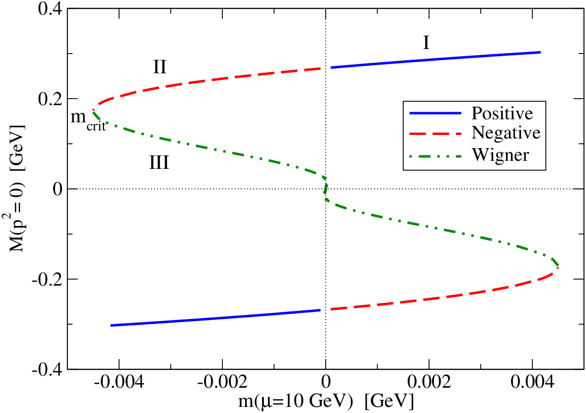


This second Wigner solution develops a total of two zero-crossings in the mass function as we cross . Increasing the mass, we follow curve ‘IV’, which again bifurcates into two solutions at some second critical mass . Continuing the procedure we follow path ‘V’ and again cross with the now characteristic development of an additional node in the mass function (see fig. 9). At this point, we make no further attempt to resolve such solutions since the critical mass now oscillates around with rapidly decreasing amplitude. We can only presume that such solutions continue to exist, with yet more nodes developing in the mass-function as the trivial solution is approached. We expect the multitude of these solutions to smoothly connect the location of the complex poles to the trivial solution, as indicated in the left diagram of fig. 9.
Once again, we point out that we did not include pion effects here, due in part to the ambiguity of choosing and for varying quark mass. Since Gribov found the same results in his approximation with the pion back-reaction [4], it seems likely that the inclusion of pions does not change this picture quantitatively.
III.3 Numerical results in the complex plane
| Vertex characterising the parabola | ||
|---|---|---|
| Schwinger function | shell method | |
| 1BC, m=0 MeV, wo | ||
| 1BC, m=3 MeV, wo | ||
| 1BC, m=0 MeV, with | ||
| 1BC, m=3 MeV, with | ||
To give a better picture on the influence of the pion back-reaction on the dressing functions at complex momentum and also to show the efficacy of the expanding shell method, detailed in section II.4 and appendix A, we show explicit solutions to the quark DSE in the complex-plane in fig. 10. For the purposes of demonstration, we employed the 1BC vertex with a small quark mass and include the contribution from the pion back-reaction.
The advantages of employing such an expanding shell method and the associated interpolation scheme becomes apparent when we use our solutions in studies of the Bethe-Salpeter equations. Not only are we able to provide solutions to the quark-DSE in the complex plane for any numerically determined gluon propagator or quark-gluon vertex – without changing or making assumptions of the analytic structure by use of fit functions – but we can do this quickly and accurately. Indeed, it is gratifying to see that our bound-state solutions change by less than a percent for a wide selection of coarse and fine grids [25].
As we expand our parabolas outward into the complex plane, our domain of exploration approaches the location of the complex poles. Close to these poles, the function becomes steep and cannot be reliably represented by our interpolation scheme without adaptive modification of the grid points. With such tuning, it is possible to see the onset of conjugate poles in the complex plane by looking for bumps arising in the solutions. Since we do not know the precise location of the pole or its residue, we cannot extend our parabolas any further. Moreover, there comes a point where the poles affect our numerical stability and lead to a breakdown of the numerical procedure.
This breakdown allows us to determine approximately on which parabola the complex poles are located, where each parabola is characterised by its vertex , the point at which the parabola crosses the real-axis. In table 2 we list the vertex of the parabolas on which the complex pole lies, as determined from the Schwinger function and as inferred by the breakdown of our numerical method. Both methods are in excellent agreement. This provided additional justification for the Fourier-transform method exploited in subsection III.1.


While this procedure can in principle be applied to the CP-vertex, whose solutions contain a pole on the negative real-axis, perhaps accompanied by a branch-cut, the numerical solution becomes much more involved due to the derivative-like terms appearing in the vertex. By implementing a robust numerical procedure that deals with this numerical singularities correctly, we believe that our method is applicable to finding solutions in the complex plane for such a vertex construction. We defer a detailed calculation to future work.
IV Conclusion
We studied the analytic structure of the quark propagator with and without the inclusion of pion effects, in order to compare and contrast with Gribov’s conjecture of quark confinement due to supercriticality of the colour charge. He advocated the viewpoint that these pions play an important rôle for the confinement of quarks, as indicated in the analytic structure of their propagator. Studying a truncation scheme that essentially includes all features introduced and studied by Gribov, we determined the unquenching effects in the quark propagator due to the back-reaction of pions onto the quarks. Our numerical results agree nicely with corresponding lattice calculations thus underlining the reliability of our truncation scheme. Investigating the analytic structure of the quark propagator by means of its Schwinger functions and direct solutions of the quark-DSE in the complex plane we found that the inclusion of pion effects had no qualitative effect. This is the central result of our work: Gribov’s conjecture does not seem to hold.
Instead, it is the relative strengths of the various tensor components that constitute the fully dressed quark-gluon vertex, in particular whether these are in agreement with those occurring in QED due to the Ward-identity. This finding is in agreement with a previous investigation of the structure of the quark propagator [12]. It relegates the question of quark confinement due to positivity violations in its Schwinger function to a more refined determination of the details of the quark-gluon vertex, see e.g. [16].
We also determined the multiple solutions of the quark-DSE as a function of the current quark mass. In the -plane we find a behaviour similar to hysteresis effects in ferromagnets connected to the phenomenon of dynamical symmetry breaking. Close to the origin of this plane we find the critical behaviour of the Wigner solution to be connected to the form of the effective running coupling associated with the quark-gluon interaction. Employing a sufficiently strong coupling with an infrared fixed point as also being used in Gribov’s work, we find a multitude of solutions near the trivial point.
Our approximation scheme for the quark-gluon interaction as a composition of a Yang-Mills part and a part due to the pion back-reaction onto the quark is a modification of the one used in [8]. This modification leads to improved values for low energy constants as the chiral condensate and the pion decay constant and therefore has the potential to describe pion cloud properties of mesons and baryons via bound state equations. This is further explored elsewhere [25].
Acknowledgements
This work has been supported by the Helmholtz-University Young Investigator Grant No VH-NG-332 and by the DFG under grant number Ni 1191/1-1.
Appendix A Solving the Quark DSE in the Complex Plane
Here we give details of our numerical method for calculating the quark DSE for complex momenta. In Euclidean space, our quark-DSE is conventionally written as
| (27) |
with the momentum flowing through the gluon. We want to solve this equation (in the previously described approximation) for complex but using real only. This also appears on consideration of the Bethe-Salpeter equations. For those we find ourselves in need of the quark propagator evaluated at momenta
| (28) |
with a momentum partitioning parameter and the total momentum of the meson. In Euclidean space, a bound state in the rest frame has total momentum and , and so the momenta of (28) define parabolic curves in the complex plane. The necessary integrals over the angles leads us to require solutions to the quark-DSE for all complex momenta bounded by these curves. For equal momentum partitioning, , the region is symmetric about the real-axis (see fig. 11 for an example). The vertex of the parabola is located at and the focus at .


In contemporary BS studies, one is generally forced to work in the rainbow-ladder approximation whereby the full quark-gluon vertex of (27) is replaced by its bare counterpart . We can then solve (27) for without iteration, requiring only as input the quark propagator on . In practice, we need only perform calculations in the upper half-plane, , since solutions are related by complex conjugation. The caveat, however, is that we require knowledge of the gluon interaction for complex momenta . In general, though the analytic structure of the gluon may be surmised, the analytic continuation of some phenomenological ansatz is at best ill-defined.
To avoid evaluating the gluon for complex momenta, we modify the momentum routing in the quark-DSE such that its momentum is manifestly real. This amounts to introducing a shift in the integration variable, , which is of course valid in any translationally invariant regularisation scheme. Such schemes are in general not employed in DSE studies, for technical reasons, so one should be mindful of any boundary terms that may arise; with a subtractive renormalisation scheme and careful consideration of the renormalisation conditions these spurious terms may be rigorously eliminated. What remains is the equation:
| (29) |
where again we consider along the parabolas of (28), and now , . Now that the integral equation depends on the a priori unknown quark propagator in the complex plane, we must employ an iterative scheme to obtain solutions.
If we choose a point that lies on a parabola with vertex at , then the integral equation only requires the quark propagator be known in the region of the complex plane bounded by the same parabola. The most efficient way to obtain solutions is then to expand in a series of parabolic shells stemming from the real-axis, as shown in fig. 12. To accelerate the iteration process, the previously converged shell is extrapolated outwards, using the Cauchy-Riemann equations, and used as an initial guess for the next shell.
Because we are dealing with complex numbers, it is necessary to employ some 2D interpolation scheme. Internally, our parabolic shells are characterised by their vertex and a parameter , shown as stacks in fig. 12, which are mapped onto the parabolas of fig. 12. It is thus straightforward to take any point and determine its corresponding value in space. Cubic-spline interpolation is used to interpolate along the closest two shells in , whilst linear interpolation in is sufficient for determining the value in-between. This essentially leads to interpolation along a parabola, such as the dashed curve shown in fig. 12.
The drawback of this approach, however, is that without precise information about the location of the poles and their residues, we are unable to explore beyond the singularities appearing in the quark propagator. This is discussed also in the main body of this work.
References
- [1] J. Greensite, Prog. Part. Nucl. Phys. 51 (2003) 1 [arXiv:hep-lat/0301023].
- [2] J. Greensite, K. Langfeld, S. Olejnik, H. Reinhardt and T. Tok, Phys. Rev. D 75 (2007) 034501 [arXiv:hep-lat/0609050].
- [3] V. N. Gribov, Eur. Phys. J. C 10, 91 (1999) [arXiv:hep-ph/9902279].
- [4] V. N. Gribov, arXiv:hep-ph/9905285.
- [5] V. Gribov, Eur. Phys. J. C 10, 71 (1999) [arXiv:hep-ph/9807224].
- [6] Y. L. Dokshitzer and D. E. Kharzeev, Ann. Rev. Nucl. Part. Sci. 54 (2004) 487 [arXiv:hep-ph/0404216].
- [7] C. Ewerz, arXiv:hep-ph/0601271;
- [8] C. S. Fischer, D. Nickel and J. Wambach, Phys. Rev. D 76 (2007) 094009 [arXiv:0705.4407 [hep-ph]].
- [9] C. S. Fischer, J. Phys. G 32, R253 (2006) [arXiv:hep-ph/0605173].
- [10] C. Ewerz, Eur. Phys. J. C 13, 503 (2000) [arXiv:hep-ph/0001038];
- [11] C. S. Fischer and R. Alkofer, Phys. Rev. D 67 (2003) 094020 [arXiv:hep-ph/0301094].
- [12] R. Alkofer, W. Detmold, C. S. Fischer and P. Maris, Phys. Rev. D 70, 014014 (2004) [arXiv:hep-ph/0309077].
- [13] D. C. Curtis and M. R. Pennington, Phys. Rev. D 42 (1990) 4165.
- [14] J. S. Ball and T. W. Chiu, Phys. Rev. D 22, 2542 (1980).
- [15] C. S. Fischer, P. Watson and W. Cassing, Phys. Rev. D 72, 094025 (2005) [arXiv:hep-ph/0509213].
- [16] R. Alkofer, C. S. Fischer and F. J. Llanes-Estrada, Mod. Phys. Lett. A 23 (2008) 1105 [arXiv:hep-ph/0607293]. R. Alkofer, C. S. Fischer, F. J. Llanes-Estrada and K. Schwenzer, Annals of Physics, in press; arXiv:0804.3042 [hep-ph].
- [17] D. Zwanziger, Phys. Rev. D 65, 094039 (2002) [arXiv:hep-th/0109224].
- [18] C. Lerche and L. von Smekal, Phys. Rev. D 65, 125006 (2002) [arXiv:hep-ph/0202194].
- [19] R. Alkofer, C. S. Fischer and F. J. Llanes-Estrada, Phys. Lett. B 611, 279 (2005) [arXiv:hep-th/0412330].
- [20] C. Kellermann and C. S. Fischer, to appear in Phys. Rev. D, arXiv:0801.2697 [hep-ph].
- [21] D. V. Shirkov and I. L. Solovtsov, Theor. Math. Phys. 150, 132 (2007) [arXiv:hep-ph/0611229].
- [22] R. Alkofer, C. S. Fischer and R. Williams, arXiv:0804.3478 [hep-ph].
- [23] W. J. Marciano and H. Pagels, Phys. Rept. 36 (1978) 137.
- [24] C. S. Fischer and R. Alkofer, Phys. Lett. B 536, 177 (2002) [arXiv:hep-ph/0202202]; A. Cucchieri and T. Mendes, PoS LATTICE, 297 (2007) [arXiv:0710.0412 [hep-lat]]; I. L. Bogolubsky, E. M. Ilgenfritz, M. Muller-Preussker and A. Sternbeck, PoS LATTICE, 290 (2007) [arXiv:0710.1968 [hep-lat]]. A. C. Aguilar, D. Binosi and J. Papavassiliou, arXiv:0802.1870 [hep-ph].
- [25] C. S. Fischer and R. Williams; in preparation
- [26] P. Maris, C. D. Roberts and P. C. Tandy, Phys. Lett. B 420 (1998) 267 [arXiv:nucl-th/9707003].
- [27] C. J. Burden, C. D. Roberts and A. G. Williams, Phys. Lett. B 285, 347 (1992).
- [28] R. Oehme, Int. J. Mod. Phys. A 10, 1995 (1995) [arXiv:hep-th/9412040].
- [29] C. J. Burden, Phys. Rev. D 57, 276 (1998) [arXiv:hep-ph/9702411]; Phys. Rev. D 59, 037502 (1999) [arXiv:hep-ph/9807438].
- [30] K. Osterwalder and R. Schrader, Commun. Math. Phys. 31 (1973) 83–112; Commun. Math. Phys. 42 (1975) 281.
- [31] V. A. Miransky, Phys. Lett. B 165, 401 (1985).
- [32] C. McNeile, Phys. Lett. B 619 (2005) 124 [arXiv:hep-lat/0504006].
- [33] P. O. Bowman, U. M. Heller, D. B. Leinweber, M. B. Parappilly, A. G. Williams and J. b. Zhang, Phys. Rev. D 71 (2005) 054507 [arXiv:hep-lat/0501019].
- [34] C. S. Fischer and M. R. Pennington, Phys. Rev. D 73, 034029 (2006) [arXiv:hep-ph/0512233].
- [35] A. Kumar, arXiv:0711.3970 [hep-th].
- [36] M. Gimeno-Segovia and F. J. Llanes-Estrada, arXiv:0805.4145 [hep-th].
- [37] L. Chang, Y. X. Liu, M. S. Bhagwat, C. D. Roberts and S. V. Wright, Phys. Rev. C 75 (2007) 015201 [arXiv:nucl-th/0605058].
- [38] R. Williams, C. S. Fischer and M. R. Pennington, Phys. Lett. B 645 (2007) 167 [arXiv:hep-ph/0612061].
- [39] P. Maris and P. C. Tandy, Phys. Rev. C 60 (1999) 055214 [arXiv:nucl-th/9905056].