Stability of the curvature perturbation in dark sectors’ mutual interacting models
Abstract
We consider perturbations in a cosmological model with a small coupling between dark energy and dark matter. We prove that the stability of the curvature perturbation depends on the type of coupling between dark sectors. When the dark energy is of quintessence type, if the coupling is proportional to the dark matter energy density, it will drive the instability in the curvature perturbations; however if the coupling is proportional to the energy density of dark energy, there is room for the stability in the curvature perturbations. When the dark energy is of phantom type, the perturbations are always stable, no matter whether the coupling is proportional to the one or the other energy density.
pacs
98.80.Cq; 98.80.-kWe are convinced by the fact that our universe is undergoing an accelerated expansion driven by the so called dark energy (DE). The leading interpretation of such a DE is the cosmological constant with equation of state (EoS) . Although the cosmological constant is consistent with the observational data, it presents apparently unsurmountable problems from the theoretical point of view, which not only requires a severe fine tuning of 120 digits to attain the actual value of the cosmological constant, but also leads to the coincidence problem, namely why the DE and the Dark Matter (DM) are comparable in size exactly today[1].
Dark Energy contributes a significant fraction of the content of the universe. It is thus natural to consider its interaction with the remaining fields of the Standard Model in the framework of standard field theory. The possibility that DE and DM can interact has been widely discussed recently [2]-[27]. It has been shown that certain types of coupling between DE and DM can lead to a late time attractor solution for the ratio of DM and DE densities [6] and provide a mechanism to alleviate the coincidence problem [2, 4]. It has been argued that an appropriate interaction between DE and DM can influence the perturbation dynamics and affect the lowest multipoles of the CMB spectrum [9, 11]. Arguments using galaxies structure formation suggested that the strength of the coupling could be as large as the QED fine structure constant [9, 12]. More recently, it was shown that such an interaction could be inferred from the expansion history of the universe, as manifested in, e.g., the supernova data together with CMB and large-scale structure information[23, 24, 16]. In addition, it was suggested that the dynamical equilibrium of collapsed structures can be affected by the coupling between DE and DM [13]. The basic idea is that the virial theorem is distorted by the non-conservation of mass caused by the coupling[22]. Thermodynamical attempts to understand the interaction between DE and DM has also been proposed [18].
Recently there has been some concern about the stability of the perturbations under DE and DM interaction [27], which could represent a sharp blade in the heart of such interacting models. In the original analysis the authors considered that the energy exchange between DE and DM is proportional to the energy densities of DM and total dark sectors. For the constant DE EOS , it was found that the instability arises regardless of how weak the coupling is. In this work we are going to reexamine the stability of the curvature perturbation when dark sectors are mutually interacting. We will concentrate on the interaction between dark sectors in a linear combination of energy densities of DE and DM, which is a more general phenomenological form in describing the interaction [29, 23]. We will restrict our investigation to constant EOS including and cases.
We consider a two-component system with each energy-momentum tensor satisfying
| (1) |
where denotes the interaction between different components and denotes either the DM or the DE sector. This equation can be projected on the time or on the space direction of the comoving observer. Using the four velocity , it can be contracted into
| (2) |
which is the projection on the time direction of the comoving observer. Above, and is the volume expansion rate. In order to get the projection along the space direction, we can use on (1) and take the contraction
| (3) |
where is the acceleration. For the homogeneous and isotropic universe, it requires . Besides, for the DM particle, its world line is the geodesic, . Thus the spacial part of vanishes, which means that in the background there is no momentum transfer between dark sectors [27]. For the whole system the energy momentum conservation still holds, satisfying , thus requiring .
We choose the perturbed space-time
| (4) |
where
| (5) |
The perturbed energy-momentum tensor reads
| (6) | |||||
regardless of the anisotropic stress, while is a new perturbation variable. Considering that the intrinsic momentum transfer can produce acoustics in the DM fluid as well as pressure which may resist the attraction of gravity and hinder the growth of gravity fluctuations during tightly coupled photon baryon period, in our study we shall neglect the intrinsic momentum transfer by setting . This is a choice of interaction and the results should not heavily depend on such assumption. Our aim is to provide examples of both stability and instability in perturbations.
We construct gauge-invariant quantities by employing Bardeen’s potentials, gauge-invariant density contrast and velocity
| (7) |
Choosing a particular gauge, the Longitudinal gauge, by defining , , one can find [28].
For the interacting model we use the perturbed pressure [27]
| (8) |
and the interaction as a linear combination of the energy densities of dark sectors,
| (9) |
where and are small positive dimensionless constants. The generality in the choice of the couplings relies on the generality of the models. In case we had a Lagrangian formulation the coupling should be fixed. Lacking a Lagrangian we are free to choose our model. We are going to show that for some choice of couplings we may achieve stability in curvature perturbations. Choosing a positive sign for the interaction the direction of the energy transfer goes from DE to DM, which is required to alleviate the coincidence problem [15] and avoid some unphysical problems such as negative DE density etc[23, 27]. In [27] it was argued that it is more natural to assume that the interaction between dark sectors depends on purely local quantities. Considering the symmetries of the Friedmann-Robertson-Walker metric, we note that the interaction can vary only in time, rather than from point to point. The only time parameter in question is the age. Thus, the factor appears in our interaction, implying that the interaction depends on the cosmic time through the global expansion rate.
By taking Fourier transformation of eq( 6), we get perturbation equations
| (10) | |||||
| (11) | |||||
| (12) | |||||
| (13) | |||||
where , . We have taken by assuming the expansion rate in the interaction to be the global expansion rate. This is a matter of choice.
In the above, . However, it is not clear what expression should we have for . In [27] it has been argued in favor of . This is correct for the scalar field, but it is not obvious for other cases, especially for a fluid with a constant equation of state. The most dangerous possibility, as far as instabilities are concerned, is since the first term in the second line of eq( 13) can lead to blow up when close to . In spite of such a danger we are considering such a case here. Assuming , , the above equations can be rewritten as
| (14) | |||||
| (15) |
By using the gauge-invariant quantity and letting we get the adiabatic initial condition,
| (16) |
The curvature perturbation relates to density contrast by [30]
| (17) |
With the help of these equations we can compute the curvature perturbation based on the CMBEASY code. We first consider the interaction between the dark sectors in proportional to the energy density of DM () and in our calculation we keep the DE EoS . For constant , we show the numerical results for the ratio in Fig.1. We observe that exhibits a scaling behavior, which keeps constant both at early and present times of the universe. This behavior is not changed when we turn on . Analytically, this can be understood by inserting the continuity equations
| (18) |
in
| (19) |
Solving the corresponding quadratic equation, we get
| (20) |
This implies
| (21) |
for . These two roots of are constant in the very early time and current time of the universe, respectively.
The scaling behavior of influences the curvature perturbation . Numerically, we see from Fig.1 that when and , blows up, which agrees with the result obtained in [27]. We find that this blow-up starts at earlier time when approaches from above and it happens regardless of the value of .
The reason for the blow up is the fact that the expression of is non perturbative in , being proportional to at very times, when we have to consider the begining of the CMB computation.


However, when we consider the dark sectors’ interaction as being proportional to the energy density of DE and examine the case that the constant EoS is a little bigger than : the blow-up disappears. Stability is also found when we extend our discussion to the constant EoS .
Numerically, we find that the first two terms on the RHS of eqs. (14) and (15) contribute more than other terms to the divergence. Using and to represent the first two terms of eq. (14), we can approximately write
| (22) |
where
| (23) |
When and , , we have one order larger than and , which causes the vast increase in as shown in Fig.2a. However, when in the case and , no matter whether or , and are of the same order as shown in Fig.2b,c and , which makes to decrease with time. Therefore, the blow up is avoided.
 |
 |
| a | b |
 |
| c |
In order to further explain the reason for the blow-up we provide an analytical analysis. Keeping the leading terms, we have the approximate equations
| (24) |
Considering the case that the interaction between dark sectors is proportional to the energy density of DM () and noting that , we can simplify the above equations to
| (25) |
A second order differential equation for is
| (26) |
In the radiation dominated period, we have and eq. (26) can be approximated as
| (27) |
whose solution is
| (28) |
where
| (29) |
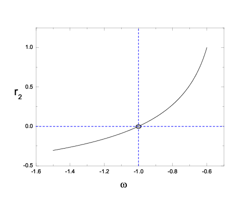
The result, eq(29), has also been given in [27], see their equations (84) and (85) by setting , putting the obvious in front of the square root and remembering . In [27], corresponds to while corresponds to . In fig.3, we see that when , both and are positive, which means that the perturbation in grows. However, when , both and are negative; this results in the decay of the perturbation in . No divergence occurs, regardless of the value of .
These results tell us that for a constant DE EoS , a coupling between DE and DM in proportional to () will lead to a violent divergence in the curvature perturbation. However, this divergence is absent for .

Considering the case that the interaction between dark sectors is proportional to the energy density of DE, namely, , eq(24) reduces to
| (30) |
We can rewrite the second order differential equation for in the form
| (31) |
In the radiation dominated era, the above equation becomes
| (32) |
Introducing the auxiliary quantities
| (33) |

we find that, when ,
| (34) |
where
| (35) |
On the other hand, when ,
| (36) |
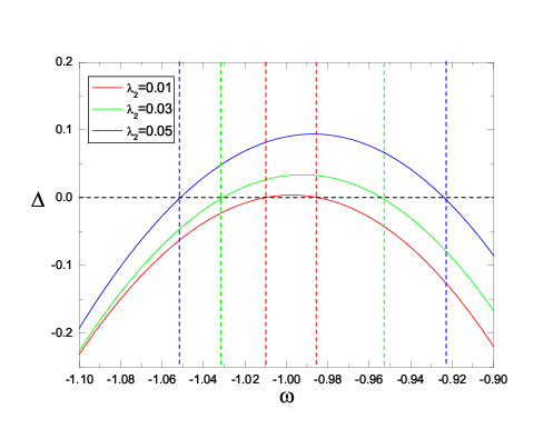
In fig. 4 we see that can be positive only in the vicinity of . When is small, the range for positive is small. is the central singularity, since it will lead to the divergence in and cause the blow-up in the density perturbation eq(34). When and , the blow-up in the density perturbation can also happen since is positive as well. But when grows further above , will become negative and so does , which will lead to the convergent result of eq(36). When , is always negative, the density perturbation will decay even when is close to from below and is small and positive.
The physical origin of such a behaviour can be traced to eq (8). When , the dark energy sound speed depends only on dark energy parameters, contrary to what happens when . In this latter case, the coupling introduces a dependence of the pressure perturbation on the dark matter energy density. In the latter case, at early times and the non-adiabatic pressure perturbation diverges at superhorizon scales, driving the instability. In our case, the effect is less acute and the system of coupled differential equations describing the evolution is better behaved.
These results show that when the interaction between dark sectors is proportional to the energy density of DE(), the blow-up in the perturbation will not happen for constant EoS . For , when the coupling is small, the blow-up can also be avoided in the observational range of the EoS. However, there is a possibility for the divergence to happen when the interaction is large in the observationally allowed range.
In summary, we have reexamined the cosmological perturbations when DE and DM interact with each other. We have specialized the interaction to be a linear combination of DE and DM energy densities, namely . We found that for constant DE EoS and nonzero the instability occurs in agreement with the results of Ref. [27]. However when and the interaction is just proportional to the energy density of DE(), the perturbation is stable for small when is within observational range. For phantom DE case with constant , the perturbation is stable regardless of the value of the coupling. This result was also evidently shown in [27]. It would be interesting to extend this study to other interaction forms. Moreover, it would be of great interest to confront the stable DE and DM interaction model to observations, such as CMB angular power and large scale structure etc. Works in these directions are in progress.
Acknowledgements.
This work has been supported partially by NNSF of China, Shanghai Science and Technology Commission and Shanghai Education Commission. The work of E. A. was supported by FAPESP and CNPQ, Brazil. B. W. would like to acknowledge D. Pavon and F. A. Barandela for helpful discussions.References
- [1] T. Padmanabhan, Phys. Rept. 380, 235 (2003); P. J. E.Peebles, B. Ratra, Rev. Mod. Phys. 75, 559 (2003); V. Sahni, Lect Notes Phys. 653:141 (2004) and references therein.
- [2] L. Amendola, Phys. Rev. D62, 043511 (2000); L. Amendola and C. Quercellini, Phys. Rev. D68, 023514 (2003); L. Amendola, S. Tsujikawa and M. Sami, Phys. Lett. B632, 155 (2006).
- [3] D. Pavón, W. Zimdahl, Phys. Lett. B628, 206 (2005).
- [4] S. Campo, R. Herrera, G. Olivares and D. Pavón, Phys. Rev. D74, 023501 (2006); S. Campo, R. Herrera and D. Pavón, Phys. Rev. D71, 123529 (2005); G. Olivares, F. Atrio-Barandela and D. Pavón, Phys. Rev. D71, 063523 (2005); S. Campo, R. Herrera, D. Pavon, Phys. Rev.D 78, 021302(R) (2008).
- [5] G. Olivares, F. Atrio-Barandela and D. Pavón, Phys. Rev. D74, 043521 (2006).
- [6] C. G. Boehmer, G. Caldera-Cabral, R. Lazkoz, R. Maartens, Phys. Rev. D 78 (2008) 023505.
- [7] B. Wang, Y. G. Gong and E. Abdalla, Phys. Lett. B624, 141 (2005).
- [8] B. Wang, C. -Y. Lin and E. Abdalla, Phys. Lett. B637, 357 (2006).
- [9] B. Wang, J. Zang, C.-Y. Lin, E. Abdalla and S. Micheletti, Nucl. Phys. B778, 69 (2007).
- [10] S. Das, P. S. Corasaniti and J. Khoury, Phys. Rev. D73, 083509 (2006).
- [11] W. Zimdahl, Int. J. Mod. Phys. D14, 2319 (2005).
- [12] E. Abdalla and B. Wang, Phys. Lett. B651, 89 (2007).
- [13] O. Bertolami, F. Gil Pedro and M. Le Delliou, Phys. Lett. B654, 165 (2007). O. Bertolami, F. Gil Pedro and M. Le Delliou, arXiv:0705.3118v1.
- [14] L. Amendola, D. Tocchini-Valentini, Phys. Rev. D 64 (2001) 043509; G. W. Anderson, S. M. Carroll, astro-ph/9711288.
- [15] W. Zimdahl, D. Pavón, L.P. Chimento, Phys. Lett. B 521 (2001) 133; L.P. Chimento, A.S. Jakubi, D. Pavón, W. Zimdahl, Phys. Rev. D 67 (2003) 083513; S. del Campo, R. Herrera, D. Pavón, Phys. Rev. D 70 (2004) 043540.
- [16] Z. K. Guo, N. Ohta and S. Tsujikawa, Phys. Rev. D76, 023508 (2007).
- [17] L. Amendola, G. Campos, R. Rosenfeld, Phys. Rev. D75, 083506 (2007).
- [18] D. Pavón, B. Wang, arXiv:0712.0565; B. Wang, C. Y. Lin, D. Pavon, E. Abdalla, Phys.Lett.B 662 1,(2008) .
- [19] G. Mangano, G. Miele and V. Pettorino, Mod. Phys. Lett. A 18, 831(2003).
- [20] B. Wang, C.-Y. Lin, D. Pavón, E. Abdalla, Phys. Lett. B662,1 (2008).
- [21] Chang Feng, Bin Wang, Yungui Gong, Ru-Keng Su , JCAP 09, 005 (2007).
- [22] E. Abdalla, L.Raul W. Abramo, L. Sodre Jr., B. Wang, arXiv:0710.1198 [astro-ph].
- [23] J. H. He, B. Wang, JCAP 06, 010 (2008), arXiv:0801.4233.
- [24] C. Feng, B. Wang, E. Abdalla, R. K. Su, Phys. Lett. B665, 111 (2008), arXiv:0804.0110.
- [25] M.R. Setare, Elias C. Vagenas Phys. Lett. B666 (2008) 111; M.R. Setare Phys. Lett. B654 (2007) 1.
- [26] B. Schaefer, G. A. Caldera-Cabral, R. Maartens, arXiv:0803.2154.
- [27] J. Valiviita, E. Majerotto, R. Maartens, JCAP 07,(2008)020, arXiv:0804.0232.
- [28] V. Mukhanov, Physical foundation of Cosmology, Cambridge University Press, (2005).
- [29] M. Quartin, M. O. Calvao, S. E. Joras, R. R. R. Reis, I. Waga, JCAP 05 (2008) 007.
- [30] H. Kodama, M. Sasaki Prog. Theor. Phys. Suppl 78 (1984) 1; C. Gordon and W. Hu Phys. Rev. D70 (2004) 083003; M. Doran A Primer on Cosmology and the Cosmic Microwave Background.