跳到论文正文
W Papers独立论文阅读器 arXiv:0807.3396 论文正文 计算阅读时间 · 0%
引用这篇论文根据当前论文元数据生成,正式投稿前建议核对。


License: arXiv.org perpetual non-exclusive license
arXiv:0807.3396v1 [cs.IT] 22 Jul 2008

Universal Denoising of Discrete-time Continuous-Amplitude Signals

Kamakshi Sivaramakrishnan † and Tsachy Weissman †    § ††thanks: Work supported in part by National Science Foundation through grants CCR-0311633 and the NSF CAREER.††thanks: †  The research was partially supported by NASA New Horizons program through grant No. 399840Q.††thanks: The material in this correspondence was presented in part at the IEEE International Symposium on Information Theory, Seattle, WA, July 2006††thanks: †  Department of Electrical Engineering, Stanford University, Stanford, CA 94305 USA (e-mails:{ksivaram,tsachy}@stanford.edu)††thanks: §  Department of Electrical Engineering, Technion – Israel Institute of Technology, Haifa, Israel.
Abstract

We consider the problem of reconstructing a discrete-time signal (sequence) with continuous-valued components corrupted by a known memoryless channel. When performance is measured using a per-symbol loss function satisfying mild regularity conditions, we develop a sequence of denoisers that, although independent of the distribution of the underlying ‘clean’ sequence, is universally optimal in the limit of large sequence length. This sequence of denoisers is universal in the sense of performing as well as any sliding window denoising scheme which may be optimized for the underlying clean signal. Our results are initially developed in a “semi-stochastic” setting, where the noiseless signal is an unknown individual sequence, and the only source of randomness is due to the channel noise. It is subsequently shown that in the fully stochastic setting, where the noiseless sequence is a stationary stochastic process, our schemes universally attain optimum performance. The proposed schemes draw from nonparametric density estimation techniques and are practically implementable. We demonstrate efficacy of the proposed schemes in denoising gray-scale images in the conventional additive white Gaussian noise setting, with additional promising results for less conventional noise distributions.

Index Terms: 
Universal Denoising, kernel density estimation, Quantization, Sliding Window Denoiser, Denoisability, Memoryless Channels, semi-stochastic setting, discrete denoising.

I Introduction

Consider the problem of estimating a clean discrete-time signal (sequence) {Xt}t∈𝕋\{X_{t}\}_{t\in\mathbb{T}}, Xt∈[a,b]⊂ℝX_{t}\in[a,b]\subset\mathbb{R}, based on its noisy observations {Zt}t∈𝕋\{Z_{t}\}_{t\in\mathbb{T}}, Zt∈ℝZ_{t}\in\mathbb{R}, where {Zt}\{Z_{t}\} is the output of a corruption mechanism, a memoryless channel. This problem finds applications in areas ranging from engineering, cryptography and statistics, to bioinformatics and beyond. There is significant literature on particular instantiations of this problem, most notably for the case where signal and noise components are real-valued and the noise is additive, most commonly Gaussian (cf. [9] and references therein). Solutions to this problem in [9] are based on wavelet-based soft thresholding and have various asymptotic optimality properties under a minimax criterion. The scope of wavelet-based thresholding in [9] has been extended beyond the additive white Gaussian case in [13], [1] where optimality is again established in an asymptotic minimax sense. The soft-thresholding scheme proposed in [1] is among the few denoisers found in the literature [13, 21] that are designed for the case of a non-Gaussian corruption mechanism. Even in this case, restrictions to additive noise and symmetry assumptions on the noise distribution are made in order to provide asymptotic performance guarantees. For the case of a random vector Y=X+ZY=X+Z, where XX is independent of ZZ (with known distribution). The Minimum Mean Squared Estimate (MMSE) of XX is well-known to be given by X^=ψ⁡(Y)=E​{X|Y}\hat{X}=\psi(Y)=E\{X|Y\}. It was shown in [27] that, for Z∼𝒩⁡(μ,Σ)Z\sim\mathcal{N}\left(\mu,\Sigma\right), ψ⁡(⋅)\psi(\cdot) satisfies ψ⁡(Y)=(Y−μ)−▽y​ln⁡fY​(Y)fY\psi(Y)=\frac{(Y-\mu)-\triangledown_{y}\ln f_{Y}(Y)}{f_{Y}}, where fY​(y)f_{Y}(y) is the marginal density of YY, which can be learned from the noisy samples Yn={Y1,⋯,Yn}Y^{n}=\{Y_{1},\cdots,Y_{n}\} of YY. Using techniques for nonparametric density estimation in [7], an estimate of fY​(y)f_{Y}(y), f^Y​(y)\hat{f}_{Y}(y), can be computed, the (appropriate) gradient of which leads to the following estimate:

ψ^​(Y)=(Y−μ)−▽y​ln⁡f^Y​(Y)f^Y\hat{\psi}(Y)=\frac{(Y-\mu)-\triangledown_{y}\ln\hat{f}_{Y}(Y)}{\hat{f}_{Y}} (1)

The authors in [27] also discuss expressions for ψ^​(Y)\hat{\psi}(Y) for a certain class of non-Gaussian noise distributions with the corruption mechanism continuing to be additive. This leaves room for universal denoising schemes for continuous valued data for a general class of noise distributions where the corruption mechanism is also arbitrary. Compression based approaches pioneered in (cf., e. g., [25] and [10]), as discussed in [36], are provably sub-optimal and suffer from non-practicality of implementation of optimal lossy compression schemes. The wavelet-based Bayesian estimation approach in [26], has demonstrated significant improvement in image denoising. However, despite much recent progress, the problem of universal denoising for discrete-time continuous-amplitude data is still a largely open problem of both theoretical and practical value. The problem is particularly relevant in new emerging areas as microarray imaging [35], array-based comparative genomic hybridization (array-CGH) [19] and medical imaging [34, 17, 22], where parametric noise models that are currently used often fail to capture the true nature of the noise.

Recently, universal denoising for discrete signals and channels was considered in [36]. The results of [36], and the denoising scheme DUDE proposed therein, although attractive theoretically, are restricted in their practicality to problems with small alphabets. This is a result of

  • •

    computational issues involved with collecting higher-order joint distributions from the noisy data.

  • •

    mapping an estimated channel output distribution to an estimated channel input distribution.

  • •

    count statistics being too sparse to be reliable for even moderately large alphabet sizes.

This leaves open challenges in the application of DUDE to problems like gray-scale image denoising. More recently, a modified DUDE, using ideas from lossless compression, was presented in [24]. As discussed in that work, in spite of circumventing some of the computational issues mentioned above, the approach leaves room for improvement in the denoising performance. The problem was further extended to the discrete-valued input and general output alphabet setting in [5]. This approach proposes quantization of the output alphabet space and proceeds on an a similar line to that in [36], showing that there is no essential loss of optimality in quantizing the channel output before denoising (insofar as learning the statistics of the underlying data is concerned). In spite of its theoretical elegance, this approach faces similar issues as the scheme of [36], limiting its scope of applications to small channel input alphabets. The authors of [5], while conjecturing the need for mild restrictions on the channel, suggest an extension of the proposed scheme to the case where both the input and output alphabet space is continuous-valued and general. The present work proposes an extension of the two-stage DUDE-like approach in [36, 5] to the case of denoising for general alphabets. A natural extension would have been to quantize both the input and the output space and apply a similar count-statistic based two-pass approach. The vast literature on nonparametric density estimation (cf. [7] and references therein), however, points to the opportunity of extracting more reliable statistics from the observed data, that would lead to better denoising (as measured under a specified loss function). We do, however, maintain the sliding window approach of [5, 36] and show asymptotic universal optimality of our schemes with increasing context lengths in the limit of large sequence lengths.

Recent developments in universal denoising in the particular context of images have also been reported in [4]. Their approach is based on local smoothing methods that make assumptions on the underlying structure of the data which are more relevant in image denoising due to the inherent redundancy of natural images. The consistency results showed the convergence of the denoising rule to the conditional expected value of the clean symbol given the noisy neighborhood sans the particular noisy symbol in question. There is potential to improve this result by incorporating the information from the noisy pixel that is being denoised too, an approach at the heart of the denoisers we present below. We establish the universal optimality of the suggested denoisers in a generality that applies to arbitrarily distributed noiseless signals, arbitrary memoryless channels, and arbitrary loss functions (with some benign regularity conditions).

The remainder of the paper is organized as follows. In section II, we discuss the problem setup and notations. This is followed by a description of the technical results that are key to the construction of the denoisers in section III. In section IV, we establish universality of a family of denoisers that we develop for the semi-stochastic setting, in which the clean data is an individual sequence and provide bounds on the difference between the performance of this proposed family of denoisers and that of the best ‘symbol-by-symbol’ denoiser chosen by a genie with full knowledge of the distribution (or probability law) of the clean data. Section V details an extension of this proposed family of denoisers to a genie that can select the best sliding window scheme, of any order, with knowledge of the underlying clean data. Section VI discusses the implication of the performance guarantees in the semi-stochastic setting to the fully stochastic setting where the clean data is generated by a stationary stochastic process, rather than an individual sequence. A slightly modified version of the proposed denoiser is shown to reduce to the scheme of [5] when the underlying clean data have finite alphabet size. The proposed family of denoisers can, hence, be seen as a natural extension of those in [5] to the current setting of denoising continuous valued symbols corrupted by a continuous memoryless channel where the clean data components may take values in a continuum. In section VII, we present some preliminary experimental results of applying the proposed schemes to denoising of gray-scale images. We conclude in section VIII with a summary of some propositions for future research directions. Throughout this paper, we maintain the flow by stating the Theorems and Lemmas corresponding to the optimality results in the main body of the paper relegating most of the proofs to the appendices.

II Problem Setting and Notations

Let 𝐱=(x1,x2,⋯)\mathbf{x}=(x_{1},x_{2},\cdots) be an individual (deterministic) noise-free source signal 11 1 throughout the paper we will be using the terms ‘signal’ and ‘sequence’ interchangeably with components taking values in [a,b]⊂ℝ[a,b]\subset\mathbb{R} and 𝐘=(Y1,Y2,⋯)\mathbf{Y}=(Y_{1},Y_{2},\cdots), Yi∈ℝY_{i}\in\mathbb{R} be the corresponding noisy observations, also referred to as the ‘output of the channel’ (corruption source). This setting, where both the underlying clean sequence and the noisy sequence are continuous valued, is the continuous-amplitude analog of the semi-stochastic setting discussed in [5]. The channel is specified by a family of distribution functions 𝒞={FY|x}x∈[a,b]\mathcal{C}=\{F_{Y|x}\}_{x\in[a,b]}, where FY|xF_{Y|x} denotes the distribution of the channel output symbol when the input symbol is xx. Also, we denote the probability measure on ℝ\mathbb{R} corresponding to FY|xF_{Y|x} by μx\mu_{x}. We make the following assumptions about the channel,

  • C1.

    A memoryless channel, which is to say that the components of 𝐘\mathbf{Y} are independent with Yi∼FY|xiY_{i}\sim F_{Y|x_{i}}.

  • C2.

    The family of measures, {μx}x∈[a,b]\{\mu_{x}\}_{x\in[a,b]}, associated with the channel, 𝒞\mathcal{C}, is uniformly tight in the sense

    supx∈[a,b]μx​([−T,T]c)→0asT→∞.\sup_{x\in[a,b]}\mu_{x}([-T,T]^{c})\rightarrow 0\quad\text{as}\quad T\rightarrow\infty.

    This condition will be needed to guarantee that one can consistently track the evolution of the marginal density of the noisy symbols at the output of the memoryless channel, regardless of the underlying 𝐱\mathbf{x}, using nonparametric Kernel density estimation techniques.

  • C3.

    The distribution functions FY|xF_{Y|x} are absolutely continuous for all x∈[a,b]x\in[a,b] w.r.t the Lebesgue measure and {fY|x}\{f_{Y|x}\} denotes the corresponding densities. This assumption is not crucial for the validity of our approach but is made for concreteness in the construction of our schemes and the development of their performance guarantees.

  • C4.

    The conditional densities of the channel form a set of linearly independent functions. This is equivalent to the “invertibility” condition of [36] which ensures that, to any distribution on the input to the channel there corresponds a unique channel output.

  • C5.

    The mapping, w.r.t a metric that will be detailed in section III, from the space of channel input distributions to the corresponding channel output distributions is continuous. The precise analytical expression describing this condition is discussed in Appendix A.

  • C6.

    The expected loss, for reasonably well-behaved loss functions (conditions L1-L2 listed subsequently in this section), induced by two output distributions that are close (under the metric discussed in section III) is continuous. Again, the analytical expression describing this condition is in the Appendix A.

The above, are rather benign conditions obeyed by most channels arising in practice, an example of this being the most commonly addressed channel, viz., the Additive White Gaussian Noise Channel (AWGN). It is easy to verify that even the multiplicative (non-additive) Gaussian channel with a finite variance and mean satisfies these requirements. In this case, the channel input (underlying clean signal) affects the variance of the channel. The fact that the underlying clean signal takes only bounded values implies that the tightness condition, C2, is satisfied. In fact, any additive noise channel with distribution functions that are absolutely continuous and the corresponding densities (of finite mean and variance) satisfying conditions C4-7 (C7 discussed in Appendix A) will satisfy the above requirements.

An n-block denoiser is a measurable mapping taking ℝn\mathbb{R}^{n} into [a,b]n[a,b]^{n}. We assume a loss function Λ:[a,b]2→[0,∞)\Lambda:[a,b]^{2}\rightarrow[0,\infty) and denote the normalized cumulative loss of an nn-block denoiser X^n\hat{X}^{n}, when the underlying sequence is xnx^{n} and the observed sequence is yny^{n}, by

LX^n​(xn,yn)=1n​∑i=1nΛ⁡(xi,X^n​(yn)​[i])L_{\hat{X}^{n}}(x^{n},y^{n})=\frac{1}{n}\sum_{i=1}^{n}\Lambda(x_{i},\hat{X}^{n}(y^{n})[i]) (2)

where X^n​(yn)​[i]\hat{X}^{n}(y^{n})[i] denotes the ii-th component of X^n​(yn)\hat{X}^{n}(y^{n}). In addition to the constraints on the channel, we impose some conditions on the permissible loss functions, Λ\Lambda. We assume the loss function, Λ\Lambda,

  1. L1.

    to be bounded,i.e., Λmax<∞\Lambda_{\max}<\infty where Λmax=supx,x^∈[a,b]Λ⁡(x,x^)\Lambda_{\max}=\sup_{x,\hat{x}\in[a,b]}\Lambda(x,\hat{x})

  2. L2.

    to be a bounded Lipschitz function. More formally, we require the Lipschitz norm, ‖Λ‖L<∞\|\Lambda\|_{L}<\infty. The Lipschitz norm of the loss function, is defined as

    ∥Λ∥L=sup0<Δ<(b−a)λ⁡(Δ)Δ\parallel\Lambda\parallel_{L}=\sup_{0<\Delta<(b-a)}\frac{\lambda\left(\Delta\right)}{\Delta} (3)

    where,

    λ(Δ,x)=supy∈[a,b]supx′:|x−x′|<Δ|Λ(x,y)−Λ(x′,y)|\lambda(\Delta,x)=\sup_{y\in[a,b]}\sup_{x^{\prime}:|x-x^{\prime}|<\Delta}\left|\Lambda(x,y)-\Lambda(x^{\prime},y)\right| (4)

    and

    λ⁡(Δ)=supx∈[a,b]λ⁡(Δ,x)\lambda\left(\Delta\right)=\sup_{x\in[a,b]}\lambda\left(\Delta,x\right) (5)

    In words, this condition necessitates continuity of the mapping that takes the estimates of the underlying symbol to the corresponding loss incurred. We require that estimates of the underlying clean symbol that are close together have corresponding loss values that are also close to each other.

It can be easily verified that the commonly used loss functions of L2L_{2}, L1L_{1} norms satisfy the aforementioned condition.

Let ℱ[a,b]\mathcal{F}^{[a,b]} denote the set of all probability distribution functions with support contained in the interval [a,b][a,b]. For F∈ℱ[a,b]F\in\mathcal{F}^{[a,b]}, we let

𝒰⁡(F)=min⁡∫x∈[a,b]x^∈[a,b]⁡Λ⁡(x,x^)​𝑑F​(x)\mathcal{U}(F)=\min_{\hat{x}\in[a,b]}\int_{x\in[a,b]}\Lambda(x,\hat{x})dF(x) (6)

denote its ‘Bayes envelope’ (our assumptions on the loss function will imply existence of the minimum). In other words, 𝒰⁡(F)\mathcal{U}(F) denotes the minimum achievable expected loss when guessing the value of X∼FX\sim F. Define the symbol-by-symbol minimum loss of xnx^{n} by

D0​(xn)=ming⁡E⁡[1n​∑i=1nΛ⁡(xi,g⁡(Yi))]D_{0}(x^{n})=\min_{g}E\left[\frac{1}{n}\sum_{i=1}^{n}\Lambda(x_{i},g(Y_{i}))\right] (7)

where the minimum is over all measurable maps g:ℝ→[a,b]g:\mathbb{R}\rightarrow[a,b]. D0​(xn)D_{0}\left(x^{n}\right) denotes the minimum expected loss in denoising the sequence xnx^{n}, using a time-invariant symbol-by-symbol rule. This can be attained by a “genie” with access to the clean sequence xnx^{n}. D0​(xn)D_{0}(x^{n}), which is the expected per-symbol loss of the optimal symbol-by-symbol rule for the individual sequence xnx^{n}, will be our benchmark for assessing the performance of the universal symbol-by-symbol denoiser that we construct in the next section. The same benchmark was used also in [5]. This is slightly different than the benchmark used in [36], which corresponded to a genie that can choose the best symbol-by-symbol rule with knowledge not only of the individual sequence xnx^{n}, but also of the noisy sequence realization YnY^{n}. The latter is irrelevant for our current setting where each of the components of YnY^{n} will take on a different value, with probability one. For xn∈[a,b]nx^{n}\in[a,b]^{n}, define

Fxn(x)=|{1≤i≤n:xi≤x}|n,F_{x^{n}}(x)=\frac{|\{1\leq i\leq n:x_{i}\leq x\}|}{n}, (8)

i.e., the CDF associated with the empirical distribution of xnx^{n}. Note that D0​(xn)D_{0}(x^{n}) can be expressed as

D0​(xn)=min⁡∫[a,b]g⁡Ex​Λ​(x,g⁡(Y))​d​FXn​(x)D_{0}(x^{n})=\min_{g}\int_{[a,b]}E_{x}\Lambda(x,g(Y))dF_{X^{n}}(x) (9)

where ExE_{x} denotes expectation when the underlying clean symbol is xx, the expectation being over the channel noise

Ex​Λ​(x,g⁡(Y))=∫Λ⁡(x,g⁡(y))​fY|x​(y)​𝑑yE_{x}\Lambda(x,g(Y))=\int\Lambda(x,g(y))f_{Y|x}(y)dy (10)

For F∈ℱ[a,b]F\in\mathcal{F}^{[a,b]}, let F⊗𝒞F\otimes\mathcal{C} and EF⊗𝒞E_{F\otimes\mathcal{C}} denote, respectively, probability and expectation when the channel input X∼FX\sim F and YY is the channel output. So that,

EF⊗𝒞​Λ​(X,g⁡(Y))\displaystyle E_{F\otimes\mathcal{C}}\Lambda(X,g(Y)) =\displaystyle= ∫[a,b]Ex​Λ​(x,g⁡(Y))​𝑑F​(x)\displaystyle\int_{[a,b]}E_{x}\Lambda(x,g(Y))dF(x) (11)
=\displaystyle= ∫[a,b][∫ℝΛ⁡(x,g⁡(y))​fY|x​(y)​𝑑y]​𝑑F​(x)\displaystyle\int_{[a,b]}\left[\int_{\mathbb{R}}\Lambda(x,g(y))f_{Y|x}(y)dy\right]dF(x)

Letting [F⊗𝒞]X|y[F\otimes\mathcal{C}]_{X|y} denote the conditional distribution of XX given Y=yY=y under F⊗𝒞F\otimes\mathcal{C}, we have

ming⁡EF⊗𝒞​Λ​(X,g⁡(Y))=EF⊗𝒞​𝒰​([F⊗𝒞]X|Y)\min_{g}E_{F\otimes\mathcal{C}}\Lambda(X,g(Y))=E_{F\otimes\mathcal{C}}\mathcal{U}\left([F\otimes\mathcal{C}]_{X|Y}\right) (12)

with 𝒰\mathcal{U} denoting the Bayes envelope as defined above. Letting gopt​[F]g_{\text{opt}}\left[F\right] denote the achiever of the minimum in (12), we note that is given by the Bayes response to [F⊗𝒞]X|y[F\otimes\mathcal{C}]_{X|y}, namely,

gopt​[F]​(y)\displaystyle g_{\text{opt}}[F](y) =\displaystyle= arg⁡min⁡∫[a,b]x^∈[a,b]⁡Λ⁡(x,x^)​d​[F⊗𝒞]X|y​(x)\displaystyle\arg\min_{\hat{x}\in[a,b]}\int_{[a,b]}\Lambda(x,\hat{x})d[F\otimes\mathcal{C}]_{X|y}(x) (13)
=\displaystyle= arg⁡min⁡∫[a,b]x^∈[a,b]⁡Λ⁡(x,x^)​fY|x​(y)​𝑑F​(x)\displaystyle\arg\min_{\hat{x}\in[a,b]}\int_{[a,b]}\Lambda(x,\hat{x})f_{Y|x}(y)dF(x)

In Lemma 12, we will establish the concavity of 𝒰⁡(F)\mathcal{U}(F), and minimizing this bounded (by our assumption of bounded Λ\Lambda) concave function over a closed compact interval, [a,b][a,b], guarantees the existence of the minimizer, goptg_{\text{opt}}. Note that from (9), (10) and (11) we have

D0​(xn)=ming⁡EFxn⊗𝒞​Λ​(X,g⁡(Y))D_{0}(x^{n})=\min_{g}E_{F_{x^{n}}\otimes\mathcal{C}}\Lambda(X,g(Y)) (14)

where FxnF_{x^{n}} was defined in (8) and the minimum is attained by gopt​[Fxn]g_{\text{opt}}\left[F_{x^{n}}\right]. Thus, only a “genie” with access to the empirical distribution of the noiseless sequence could employ gopt​[Fxn]g_{\text{opt}}[F_{x^{n}}].

III Construction of Universal ‘Symbol-by-symbol’ Denoiser and Preliminaries

FxnF_{x^{n}} and, hence, gopt​[Fxn]g_{\text{opt}}[F_{x^{n}}] are not known to an observer of the noisy sequence. The first step towards constructing an estimate of gopt​[Fxn]g_{\text{opt}}[F_{x^{n}}] is to estimate the input empirical distribution from the observable noisy sequence, YnY^{n}, and knowledge of the channel, 𝒞\mathcal{C}. We approach this problem by first estimating a function that tracks the evolution of the ‘average’ density function according to which the noisy symbols are distributed. For an input sequence xnx^{n}, given the memoryless nature of the channel, the output symbols will be independent with respective distributions, {FY|x1,⋯,FY|xn}\{F_{Y|x_{1}},\cdots,F_{Y|x_{n}}\} and have the corresponding density functions, {fY|x1,⋯,fY|xn}\{f_{Y|x_{1}},\cdots,f_{Y|x_{n}}\}. The function we are interested in estimating is

fYn​(y)=1n​∑i=1nfY|xi​(y)f_{Y}^{n}(y)=\frac{1}{n}\sum_{i=1}^{n}f_{Y|x_{i}}(y) (15)

which can be thought of as the marginal density, fYnf_{Y}^{n}, of the noisy symbols in the semi-stochastic setting where xnx^{n} is the unknown deterministic sequence. The estimation of this function is done by exploiting the vast literature on density estimation techniques [7], [6], the details of which are discussed in Subsection III-A below. Once we have an estimate fYn=fYn​[Yn]f_{Y}^{n}=f_{Y}^{n}[Y^{n}] for this function, we use it to estimate the input empirical distribution by

F^xn​[Yn]=arg⁡minF∈ℱn[a,b]⁡d⁡(fYn,∫fY|x​dF​(x)⏟[F⊗𝒞]Y)\hat{F}_{x^{n}}[Y^{n}]=\arg\min_{F\in\mathcal{F}^{[a,b]}_{n}}d\left(f_{Y}^{n},\underbrace{\int f_{Y|x}dF(x)}_{[F\otimes\mathcal{C}]_{Y}}\right) (16)

where ℱn[a,b]⊆ℱ[a,b]\mathcal{F}_{n}^{[a,b]}\subseteq\mathcal{F}^{[a,b]} denotes the set of empirical distributions induced by nn-tuples with [a,b][a,b]-valued components and [F⊗𝒞]Y\left[F\otimes\mathcal{C}\right]_{Y} denotes the marginal density induced at the output of the channel by an input distribution FF. That is, every member, F⁡(x)F(x), of ℱn[a,b]\mathcal{F}_{n}^{[a,b]} is of the form

F⁡(x)=1n​∑i=1n𝟏(x≤xi)F(x)=\frac{1}{n}\sum_{i=1}^{n}\mathbf{1}_{(x\leq x_{i})} (17)

for some nn-tuple, xn=(x1,x2,⋯,xn)x^{n}=\left(x_{1},x_{2},\cdots,x_{n}\right), with [a,b][a,b]-valued components. The norm, dd, in (16) is defined as

d⁡(f,g)=∫|f⁡(y)−g⁡(y)|​𝑑yd\left(f,g\right)=\int\left|f(y)-g(y)\right|dy (18)

The channel, 𝒞\mathcal{C}, induces a set of ‘feasible’ densities of the output noisy symbol corresponding to the family of empirical distributions of the underlying clean sequence at the input of the channel. The density estimate, fYnf_{Y}^{n}, which is constructed only from the noisy sequence, YnY^{n}, is oblivious to the set of achievable marginal densities and hence could lie outside this set. It is thus natural to estimate the unobserved FxnF_{x^{n}} by the member of ℱn[a,b]\mathcal{F}_{n}^{[a,b]} leading to a channel output distribution closest to the estimated one, fYnf_{Y}^{n}. This is exactly the estimate in (16). The uniqueness of the minimizer in (16) follows from the fact that the objective function being minimized is a norm-function and hence convex, coupled with the linear independence assumption of the channel, C4. The assumption, C4, implies a one-to-one correspondence between channel input and channel output distributions (i.e., “invertibility” of the channel). Additionally, the search for the minimizer is conducted on a convex set of distribution functions, ℱn[a,b]\mathcal{F}^{[a,b]}_{n}, resulting in uniquely achieving the minimizer or in other words, the candidate input empirical distribution estimate.

A two-stage quantization of both, the support of the underlying clean symbol, [a,b][a,b], and the levels of the estimate of its empirical distribution function, F^xn\hat{F}_{x^{n}}, is carried out to give the corresponding quantized probability mass function that has mass points only at the quantized symbols.

  • Q1.

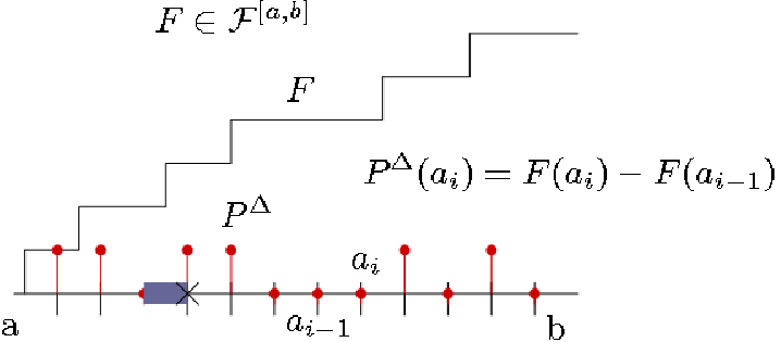
    The quantization of the interval [a,b][a,b] is depicted in Fig. 1 below.

    Refer to caption
    Fig. 1: Quantization of the support of a distribution function, F∈ℱ[a,b]F\in\mathcal{F}^{[a,b]}

    For a given quantization step size, Δ\Delta, the quantized symbols, aia_{i} in the interval [a,b][a,b] are constructed in the following manner.
    For Δ>0\Delta>0, N⁡(Δ)=(b−a)ΔN(\Delta)=\frac{(b-a)}{\Delta}, if m=⌊b−aΔ⌋m=\lfloor\frac{b-a}{\Delta}\rfloor, consider a family of vectors,

    ℱΔ={PΔ:PΔ=(P⁡(a0),P⁡(a1),⋯,P⁡(aN⁡(Δ)))}𝒜Δ={ai=a+i​Δ,i=0,⋯,N⁡(Δ)}s.t. ∑i=1N⁡(Δ)P⁡(ai)=1\begin{split}\mathcal{F}^{\Delta}&=\{P^{\Delta}:P^{\Delta}=\left(P(a_{0}),P(a_{1}),\cdots,P(a_{N\left(\Delta\right)})\right)\}\\ \mathcal{A}^{\Delta}&=\{a_{i}=a+i\Delta,i=0,\cdots,N(\Delta)\}\\ &\text{s.t. }\quad\sum_{i=1}^{N(\Delta)}P(a_{i})=1\end{split}

    else, define the family of vectors as ℱΔ={PΔ\mathcal{F}^{\Delta}=\{P^{\Delta}: PΔ=(P⁡(a0),P⁡(a1),⋯,P⁡(aN⁡(Δ)−1)CLOSE,P^{\Delta}=\left(P(a_{0}),P(a_{1}),\cdots,P(a_{N\left(\Delta\right)-1}),\right. P(aN⁡(Δ)))}\left.P(a_{N\left(\Delta\right)})\right)\}, 𝒜Δ={ai=a+i​Δ,i=0,⋯,N⁡(Δ)−1},aN⁡(Δ)=b,∑i=1N⁡(Δ)P⁡(ai)=1\mathcal{A}^{\Delta}=\{a_{i}=a+i\Delta,i=0,\cdots,N(\Delta)-1\},a_{N(\Delta)}=b,\sum_{i=1}^{N(\Delta)}P(a_{i})=1.
    As indicated in Fig. 1, the probability mass function, PΔP^{\Delta}, that we propose is constructed by allocating the mass of the distribution function, FF, in any quantization interval (of length Δ\Delta) to the higher end point in that interval. More precisely,

    PΔ​(ai)=F⁡(ai)−F⁡(ai−1)P^{\Delta}(a_{i})=F(a_{i})-F(a_{i-1}) (19)

    where aia_{i}’s as defined above and note that

    PΔ​(B)\displaystyle P^{\Delta}\left(B\right) =\displaystyle= ∑ai∈BP⁡(ai)\displaystyle\sum_{a_{i}\in B}P(a_{i})

    with any B∈ℬ[a,b]B\in\mathcal{B}^{[a,b]}, ℬ[a,b]\mathcal{B}^{[a,b]} is the Borel sigma-algebra generated by open sets in [a,b][a,b].

    Applying this quantization of the support of the underlying clean symbol to the estimate, F^xn\hat{F}_{x^{n}}, we construct now, the corresponding probability mass function, P^xnΔ\hat{P}_{x^{n}}^{\Delta}

    P^xnΔ​(ai)=F^xn​(ai)−F^xn​(ai−1)\hat{P}_{x^{n}}^{\Delta}(a_{i})=\hat{F}_{x^{n}}(a_{i})-\hat{F}_{x^{n}}(a_{i-1}) (20)

    where, ai∈𝒜Δa_{i}\in\mathcal{A}^{\Delta}.

  • Q2.

    The quantization of the values P^xn\hat{P}_{x^{n}} is carried out using a uniform quantizer, QδQ_{\delta}

    P^xnδ,Δ=Qδ​(P^xnΔ)\hat{P}^{\delta,\Delta}_{x^{n}}=Q_{\delta}(\hat{P}^{\Delta}_{x^{n}}) (21)

    where, δ\delta denotes the quantization step-size on the interval [0,1][0,1].

This is primarily motivated by tractability of the proof of the asymptotic optimality results. But, it can also be argued that any practical implementation of this proposed denoiser only has a finite precision representation of the underlying clean symbol and the distribution function values itself. Analysis of the asymptotic optimality results also lends itself nicely to viewing the distribution of the underlying clean symbol, F^xn\hat{F}_{x^{n}}, as the asymptotic limit attained by its quantized, finite precision representation, P^xnδ,Δ\hat{P}^{\delta,\Delta}_{x^{n}}. This is formalized in section III-C where we discuss the precise convergence notion of P^xnΔ\hat{P}^{\Delta}_{x^{n}} to the un-quantized probability measure.

The minimizer of the Bayes envelope in (13) is then constructed from the quantized probability mass function, Pxnδ,ΔP_{x^{n}}^{\delta,\Delta},as gopt​[Pxnδ,Δ]g_{\text{opt}}\left[P_{x^{n}}^{\delta,\Delta}\right], where goptg_{\text{opt}} for the quantized clean symbol is,

gopt​[P]​(y)\displaystyle g_{\text{opt}}[P](y) =\displaystyle= arg⁡minx^∈𝒜Δ​∑a∈𝒜ΔΛ⁡(a,x^)⋅fY|x=a​(y)⋅P⁡(X=a)\displaystyle\arg\min_{\hat{x}\in\mathcal{A}^{\Delta}}\sum_{a\in\mathcal{A}^{\Delta}}\Lambda\left(a,\hat{x}\right)\cdot f_{Y|x=a}(y)\cdot P\left(X=a\right) (22)

𝒜Δ\mathcal{A}^{\Delta} is finite alphabet approximation of [a,b][a,b] corresponding to the quantization step size of Δ\Delta. Note that we have extended the definition of goptg_{\text{opt}} to accommodate the case when PP is not a valid probability, i.e., P^xnδ,Δ\hat{P}_{x^{n}}^{\delta,\Delta} (it does not sum up to 1). Equipped with P^xnδ,Δ\hat{P}_{x^{n}}^{\delta,\Delta}, the candidate for the nn-block symbol-by-symbol denoiser is now given by

X~n,δ,Δ​[yn]​(i)=gopt​[P^xnδ,Δ​[yn]]​(yi),1≤i≤n\tilde{X}^{n,\delta,\Delta}[y^{n}](i)=g_{\text{opt}}\left[\hat{P}^{\delta,\Delta}_{x^{n}}[y^{n}]\right](y_{i}),\qquad 1\leq i\leq n (23)

where, goptg_{\text{opt}} is given in (22). We now proceed to discuss in detail the construction and consistency results of the estimate, fYnf_{Y}^{n}, F^xn\hat{F}_{x^{n}} and its quantized version, P^xnδ,Δ\hat{P}^{\delta,\Delta}_{x^{n}}.

III-A Density Estimation for independent and non identically distributed random variables

We now obtain an estimator fYnf_{Y}^{n}, for the function in (15) which depends on xnx^{n} and therefore unknown to the denoiser. Given the memoryless nature of the channel, the sequence of output symbols, Y1,Y2,⋯,YnY_{1},Y_{2},\cdots,Y_{n} are independent random variables taking values in ℝ\mathbb{R}, having conditional densities, fY|x1,fY|x2,⋯,fY|xnf_{Y|x_{1}},f_{Y|x_{2}},\cdots,f_{Y|x_{n}} respectively. A density estimate is a sequence f1,f2,⋯,fnf^{1},f^{2},\cdots,f^{n}, where for each nn, fYn​(y)=fn​(y,Y1,⋯,Yn)f^{n}_{Y}(y)=f^{n}(y;Y_{1},\cdots,Y_{n}) is a real-valued Borel measurable function of its arguments, and for fixed nn, fnf^{n} is a density estimate on ℝ\mathbb{R}. The kernel density estimate is given by

fYn​(y)=1n​hd​∑i=1nK⁡(y−Yih)f^{n}_{Y}(y)=\frac{1}{nh^{d}}\sum_{i=1}^{n}K\left(\frac{y-Y_{i}}{h}\right) (24)

where h=hnh=h_{n} is a sequence of positive numbers and KK is a Borel measurable function satisfying K≥0K\geq 0, ∫K=1\int K=1. The L1L_{1} distance, JnJ_{n}, is defined as

Jn=∫|fYn​(y)−1n​∑i=0nfY|xi​(y)|​𝑑yJ_{n}=\int\left|f^{n}_{Y}(y)-\frac{1}{n}\sum_{i=0}^{n}f_{Y|x_{i}}(y)\right|dy (25)

The choice of L1L_{1} distance as elaborated by the authors in [7] is motivated by its invariance under monotone transformations of the coordinate axes and the fact that it is always well-defined. Before proceeding to discuss convergence results for JnJ_{n}, we present definitions of certain types of kernel functions, KK, that are the backbone to kernel density estimation techniques, [6].

Definition 1

The class of kernels, 𝒦\mathcal{K} s.t. ∀K∈𝒦\forall K\in\mathcal{K}, we have

∫K=1\displaystyle\int K=1

and KK is symmetric about 00 are called class 0 kernels.

Definition 2

A class s kernel is a class 0 kernel for which

∫|x|s​|K⁡(x)|​𝑑x<∞\displaystyle\int|x|^{s}|K(x)|dx<\infty

and

∫xi​K​(x)​𝑑x=0\displaystyle\int x^{i}K(x)dx=0

for all i=1,⋯,s−1i=1,\cdots,s-1. Most class 0 kernels are in fact class 2 kernels, the only additional condition being that ∫|x|2​K​(x)<∞\int|x|^{2}K(x)<\infty. However, nonnegative class 0 kernels cannot possibly of class s≥3s\geq 3.

Theorem 1

Let KK be a nonnegative Borel measurable function on ℝ\mathbb{R} with ∫K=1\int K=1 of class s=2s=2. Let fYnf^{n}_{Y} be the kernel estimate in (24) and JnJ_{n}, the corresponding error as defined in (25). Consider

  1. 1.

    Jn→0J_{n}\rightarrow 0 in probability as n→∞n\rightarrow\infty, for some sequence 𝐱=(x1,x2,⋯)\mathbf{x}=(x_{1},x_{2},\cdots)

  2. 2.

    Jn→0J_{n}\rightarrow 0 in probability as n→∞n\rightarrow\infty, for all sequences 𝐱=(x1,x2,⋯)\mathbf{x}=(x_{1},x_{2},\cdots)

  3. 3.

    Jn→0J_{n}\rightarrow 0 almost surely as n→∞n\rightarrow\infty, for all sequences 𝐱=(x1,x2,⋯)\mathbf{x}=(x_{1},x_{2},\cdots)

  4. 4.

    For all ϵ>0\epsilon>0, there exist rr, n0>0n_{0}>0 such that P⁡(Jn≥ϵ)≤e−r​nP(J_{n}\geq\epsilon)\leq e^{-rn}, n≥n0n\geq n_{0}, for all sequences 𝐱\mathbf{x}.

  5. 5.

    limn→∞h=0\lim_{n\rightarrow\infty}h=0, limn→∞n​h=∞\lim_{n\rightarrow\infty}nh=\infty

Then, 5 ⇒\Rightarrow 4 ⇒\Rightarrow 3 ⇒\Rightarrow 2 ⇒\Rightarrow 1.

The following lemma is key to the proof of Theorem 1.

Lemma 1

For any family of channel probability density functions,
{fY|x}x∈[a,b]\{f_{Y|x}\}_{x\in[a,b]} on ℝ\mathbb{R}, satisfying assumptions C1-C7, and any non-negative, integrable function KK, with ∫K⁡(x)​𝑑x=1\int K(x)dx=1, condition 4) in Theorem 1 holds whenever

limn→∞hn=0​ and ​limn→∞n​hd=∞\lim_{n\rightarrow\infty}h_{n}=0\mbox{ and }\lim_{n\rightarrow\infty}nh^{d}=\infty (26)
Proof:

The implication that 5 ⇒\Rightarrow 4 is proved in Lemma 26. Since clearly, 4 ⇒\Rightarrow 3 ⇒\Rightarrow 2 ⇒\Rightarrow 1, the proof of Theorem 1 is complete. ∎

III-B Channel Inversion

The mapping in (16) projects the kernel density estimate of 1n​∑i=1nfY|xi​(y)\frac{1}{n}\sum_{i=1}^{n}f_{Y|x_{i}}(y) to an estimate of the empirical distribution, FxnF_{x^{n}}. This projection is such that it best approximates (in the L1L_{1} sense), the kernel density estimate with a member in the set of achievable channel output distributions. From the construction of fYnf_{Y}^{n} in (24), it is clear that fYnf_{Y}^{n} is a bona fide density on ℝ\mathbb{R}. Additionally, from the construction of F^xn\hat{F}_{x^{n}} in (16), we see that for every F∈ℱn[a,b]F\in\mathcal{F}_{n}^{[a,b]}, [F⊗𝒞]Y\left[F\otimes\mathcal{C}\right]_{Y} is also a valid density in ℝ\mathbb{R}. Finally, from the definition of the norm, dd, in (18), it is true that for fYnf_{Y}^{n} and [F⊗𝒞]Y[F\otimes\mathcal{C}]_{Y} being bona fide densities on ℝ\mathbb{R}, 0≤d⁡(fYn,[F⊗𝒞]Y)≤20\leq d\left(f_{Y}^{n},[F\otimes\mathcal{C}]_{Y}\right)\leq 2, ∀\forall, nn. These facts, together with the convexity of ℱn[a,b]\mathcal{F}_{n}^{[a,b]} show that the estimator in (16) is well defined. With the Levy metric defined as:

Definition 3 (Levy metric)

The Levy distance λ⁡(F,G)\lambda\left(F,G\right) between any two distributions FF and GG is defined as

λ⁡(F,G)=inf{ε>0:F⁡(x−ε)−ε≤G⁡(x)≤F⁡(x+ε)+ε​ for all ​x}\lambda\left(F,G\right)=\inf\{\varepsilon>0:F(x-\varepsilon)-\varepsilon\leq G(x)\leq F(x+\varepsilon)+\varepsilon\text{ for all }x\}

we have:

Theorem 2

For the estimator, F^xn\hat{F}_{x^{n}} defined in equation (16) we have λ⁡(Fxn,F^xn)→0\lambda\left(F_{x^{n}},\hat{F}_{x^{n}}\right)\rightarrow 0 a.s. for all 𝐱∈[a,b]∞\mathbf{x}\in[a,b]^{\infty}

The proof of Theorem 2 is discussed in detail in the Appendix C.

III-C Distribution-independent Approximation of the Estimate of the Input empirical distribution

In this section, we discuss the convergence notion of P^xnΔ\hat{P}_{x^{n}}^{\Delta} to the law corresponding to the un-quantized distribution function F^xn\hat{F}_{x^{n}}.

Definition 4 (β\beta metric)

For any two laws PP and QQ on SS, f:S→ℝf:S\rightarrow\mathbb{R} let ∫f​d​(P−Q):=∫f​𝑑P−∫f​𝑑Q\int fd\left(P-Q\right):=\int fdP-\int fdQ, for bounded ∫f​𝑑P\int fdP and ∫f​𝑑Q\int fdQ, the Prohorov metric is defined as

β(P,Q)=sup{|∫fd(P−Q)|:∥f∥B​L≤1}\beta\left(P,Q\right)=\sup\left\{\left|\int fd\left(P-Q\right)\right|:\parallel f\parallel_{BL}\leq 1\right\}

where

∥f∥B​L=∥f∥L+∥f∥∞\parallel f\parallel_{BL}=\parallel f\parallel_{L}+\parallel f\parallel_{\infty} (27)

and

∥f∥L=:=supx≠y|f⁡(x)−f⁡(y)||x−y|,∥f∥∞=supx|f(x)|\parallel f\parallel_{L}=:=\sup_{x\neq y}\frac{\left|f(x)-f(y)\right|}{|x-y|},\qquad\parallel f\parallel_{\infty}=\sup_{x}\left|f(x)\right| (28)

Equipped with this definition, we now state the following theorem,

Theorem 3
limΔ→∞β⁡(P^xn,P^xnΔ)=0\lim_{\Delta\rightarrow\infty}\beta\left(\hat{P}_{x^{n}},\hat{P}_{x^{n}}^{\Delta}\right)=0 (29)

where, P^xn\hat{P}_{x^{n}} denotes the law associated with the distribution function F^xn\hat{F}_{x^{n}}.

Proof:

Follows directly from Lemma 2.
∎

Lemma 2

For any F∈ℱ[a,b]F\in\mathcal{F}^{[a,b]},

limΔ→0β⁡(P,PΔ)=0\lim_{\Delta\rightarrow 0}\beta\left(P,P^{\Delta}\right)=0 (30)

where PP is the law associated with distribution functions in the family ℱ[a,b]\mathcal{F}^{[a,b]}. Particularly, the FF and PΔP^{\Delta} that satisfies (30) is defined by,

PΔ​(ai)=F⁡(ai)−F⁡(ai−1)P^{\Delta}(a_{i})=F(a_{i})-F(a_{i-1}) (31)

where ai∈𝒜Δa_{i}\in\mathcal{A}^{\Delta} and 𝒜Δ\mathcal{A}^{\Delta} is the finite alphabet approximation of [a,b][a,b] discussed earlier.

In words, any empirical distribution of the underlying clean sequence is approximated arbitrarily well with a PMF on the quantized set of points when the quantization is fine enough.

Next we discuss the mechanics of the construction of the denoiser, which has the density estimation and the channel inversion steps as its core.

III-D Implementation of the symbol-by-symbol denoiser

The implementation of the denoiser in the previous section involves a discretization of the density estimation and the channel inversion steps. The discretized version of the kernel density estimate, fYn​(y)f^{n}_{Y}(y), in (24) is evaluated at a set of discrete points, {y1,⋯,yN}\{y_{1},\cdots,y_{N}\} . This gives an NN-dimensional vector of the distribution function, pYn​(y)p^{n}_{Y}(y). The “channel inversion” in (16) is also discretized using the estimate, pYn​(y)p^{n}_{Y}(y).

III-D1 Fast kernel density estimation

The Kernel density estimation in (24) for a given kernel function, KK, although simple in construction, is faced with a significant computational burden for a brute-force computation of O⁡(N​n)O(Nn) corresponding to nn data points and NN points {y1,⋯,yN}\{y_{1},\cdots,y_{N}\} at which pYn​(y)p_{Y}^{n}(y) is evaluated. The computational complexity can be greatly reduced by using FFT based methods [31]. Recently, there has been extensive work on the use of fast gauss transform-based techniques [16] for reduction of computational complexity. These techniques reduce the complexity from O⁡(N​n)O(Nn) to O⁡(N+n)O(N+n). The cardinal factor in nonparametric density estimation procedures is the choice of the optimal bandwidth, hh, in (24). There has been some recent work in [14] on using dual-tree methods to derive fast methods for optimal bandwidth choice that continues to maintain the complexity of this step at O⁡(N+n)O(N+n). For N=O⁡(n)N=O(n), this reduces to O⁡(n)O(n).

III-D2 Channel inversion using linear programming techniques

In solving the channel inversion problem in (16), we are looking for a vector in the probability simplex, ℱΔ={P:∑i=1N⁡(Δ)P(ai),ai∈𝒜Δ}\mathcal{F}^{\Delta}=\{P:\sum_{i=1}^{N\left(\Delta\right)}P\left(a_{i}\right),a_{i}\in\mathcal{A}^{\Delta}\}, for our candidate distribution function, P^xnδ,Δ\hat{P}_{x^{n}}^{\delta,\Delta}. The discretized version of (16) is given by,

P^xnδ,Δ=arg⁡min⁡∑i=1Np∈ℱΔ⁡|pYn​(yi)−∑j=1N⁡(Δ)fY|x=xj​(yi)​Qδ​(p⁡(xj))|\hat{P}_{x^{n}}^{\delta,\Delta}=\arg\min_{p\in\mathcal{F}^{\Delta}}\sum_{i=1}^{N}\left|p^{n}_{Y}(y_{i})-\sum_{j=1}^{N(\Delta)}f_{Y|x=x_{j}}(y_{i})Q_{\delta}\left(p\left(x_{j}\right)\right)\right| (32)

The objective function, being an L1L_{1}-norm, is clearly a convex function (of the input distribution, p⁡(⋅)p(\cdot)) and the candidate minimizer also resides in the convex subspace, viz., the probability simplex ℱΔ\mathcal{F}^{\Delta}. This can be easily solved using well-studied linear programming algorithms in the broader area of convex optimization techniques. The particular reformulation of the problem solved is of the form

P^xnδ,Δ\displaystyle\hat{P}_{x^{n}}^{\delta,\Delta} =\displaystyle= arg⁡min⁡∑i=1Np∈ℱΔ⁡εi\displaystyle\arg\min_{p\in\mathcal{F}^{\Delta}}\sum_{i=1}^{N}\varepsilon_{i}
s.t. pYn​(yi)−∑j=1N⁡(Δ)fY|x=xj​(yi)​Qδ​(p⁡(xj))≤εi\displaystyle p^{n}_{Y}(y_{i})-\sum_{j=1}^{N(\Delta)}f_{Y|x=x_{j}}(y_{i})Q_{\delta}\left(p(x_{j})\right)\leq\varepsilon_{i} (33)
∑j=1N⁡(Δ)fY|x=xj​(yi)​Qδ​(p⁡(xj))−pYn​(yi)≤εi∀i∈{1,⋯,N}\displaystyle\sum_{j=1}^{N(\Delta)}f_{Y|x=x_{j}}(y_{i})Q_{\delta}\left(p(x_{j})\right)-p^{n}_{Y}(y_{i})\leq\varepsilon_{i}\qquad\forall i\in\{1,\cdots,N\}

The computational complexity of solving this problem using the popular interior point methods [2] is O⁡((N+N⁡(Δ))3)=O⁡((N+1Δ)3)=O⁡((N+log⁡n)3)O((N+N(\Delta))^{3})=O\left((N+\frac{1}{\Delta})^{3}\right)=O((N+\log n)^{3}). This again, for N=O⁡(n)N=O(n), reduces to O⁡((n+log⁡n)3)=O⁡(n3)O\left(\left(n+\log n\right)^{3}\right)=O(n^{3}).

The two-pronged quantization discussed in the previous section can be naturally built into the optimization problem in (32) by searching in

ℱδ,Δ={Qδ​(P):P∈ℱΔ}\mathcal{F}^{\delta,\Delta}=\left\{Q_{\delta}(P):P\in\mathcal{F}^{\Delta}\right\} (34)

the set of N⁡(Δ)N\left(\Delta\right)-tuples with components in [0,1] that are integer multiples of 1δ\frac{1}{\delta} with point masses on the set 𝒜Δ\mathcal{A}^{\Delta}. The formulation would then be

P^xnδ,Δ\displaystyle\hat{P}_{x^{n}}^{\delta,\Delta} =\displaystyle= arg⁡min⁡∑i=1Np∈ℱδ,Δ⁡εi\displaystyle\arg\min_{p\in\mathcal{F}^{\delta,\Delta}}\sum_{i=1}^{N}\varepsilon_{i}
s.t. pYn​(yi)−∑j=1N⁡(Δ)fY|x=xj​(yi)​p​(xj)≤εi\displaystyle p^{n}_{Y}(y_{i})-\sum_{j=1}^{N(\Delta)}f_{Y|x=x_{j}}(y_{i})p(x_{j})\leq\varepsilon_{i}
∑j=1N⁡(Δ)fY|x=xj​(yi)​p​(xj)−pYn​(yi)≤εi∀i∈{1,⋯,N}\displaystyle\sum_{j=1}^{N(\Delta)}f_{Y|x=x_{j}}(y_{i})p(x_{j})-p^{n}_{Y}(y_{i})\leq\varepsilon_{i}\qquad\forall i\in\{1,\cdots,N\}

This channel inversion is at the heart of the denoiser in (22) and its simple formulation makes the scheme particularly elegant and practically implementable. The estimate of the empirical distribution in (32) is then plugged into (22) to finally give an estimate of the underlying clean symbol according to (23). The denoiser is described as Algorithm 1 below.

input : Noisy sequence yny^{n}, channel 𝒞\mathcal{C}
output : Denoised sequence, x^n\hat{x}^{n}
FIRST PASS
Density estimation step
input : Noisy sequence, yny^{n}
output : Density estimate, fYnf^{n}_{Y}
Determine the optimal bandwidth from any one of the techniques discussed in [31], e.g., cross-validation
Use techniques discussed in [14] for fast evaluation of (24)
Channel inversion step
input : fYnf_{Y}^{n}, Quantization resolutions, δ\delta,Δ\Delta
output : P^xnδ,Δ\hat{P}_{x^{n}}^{\delta,\Delta}
Construct an LP (Linear Program) as in (33) and use linprog (in MATLAB) or any complex program solver to solve it. Alternatively, use log-barrier methods discussed in [3] to solve for the estimate, F^xn\hat{F}_{x^{n}}
Use the quantization mapping in (20) to map F^xn\hat{F}_{x^{n}} to P^xnΔ\hat{P}_{x^{n}}^{\Delta}
Then use a uniform quantizer with resolution δ\delta to get P^xnδ,Δ←Qδ​(P^xnΔ)\hat{P}_{x^{n}}^{\delta,\Delta}\leftarrow Q_{\delta}\left(\hat{P}_{x^{n}}^{\Delta}\right)
SECOND PASS
input : Noisy sequence, yny^{n}, channel 𝒞\mathcal{C}, estimate of input distribution P^xnδ,Δ\hat{P}_{x^{n}}^{\delta,\Delta}
output : Denoised Sequence, x^n\hat{x}^{n}
Use equation (22), (23) to denoise at every location, ii
for i←1i\leftarrow 1 to nn do  x^i←gopt​[P^xnδ,Δ]​(yi)\hat{x}_{i}\leftarrow g_{\text{opt}}[\hat{P}^{\delta,\Delta}_{x^{n}}](y_{i}) end
Algorithm 1 Symbol-by-symbol denoiser in Section III

IV Performance guarantees for the Symbol by Symbol denoiser

The main result of this section is Theorem 43 below, which establishes the universal asymptotic optimality of our proposed symbol-by-symbol denoiser in (23) with respect to the class of symbol-by-symbol schemes. The predominant technical result leading to Theorem 43 is Theorem 4. We continue to restrict ourselves to the semi-stochastic setting where the underlying clean sequence is an unknown, but deterministic, sequence 𝐱\mathbf{x}. The benchmark performance for the clean sequence is the minimum possible symbol-by-symbol loss, D0​(xn)D_{0}\left(x^{n}\right), defined in Section II. Theorem 43 shows that our proposed denoiser, gopt​[P^xnδ,Δ]g_{\text{opt}}\left[\hat{P}_{x^{n}}^{\delta,\Delta}\right], asymptotically (as the number of observations increases) achieves that benchmark performance. This is achieved by bounding the deviation of the cumulative loss incurred by gopt​[P^xnδ,Δ]g_{\text{opt}}\left[\hat{P}_{x^{n}}^{\delta,\Delta}\right] from the minimum possible symbol-by-symbol loss in Theorem 4 for any block length, nn. Hence we show that, gopt​[P^xnδ,Δ]g_{\text{opt}}\left[\hat{P}_{x^{n}}^{\delta,\Delta}\right] performs essentially as well as the best possible symbol-by-symbol denoiser, D0​(xn)D_{0}\left(x^{n}\right).

In preparation for Theorem 4 let ℱδ,Δ\mathcal{F}^{\delta,\Delta}, defined in (34), denote the set of probabilities with components in [0,1] that are integer multiples of δ\delta (defined under Q2. in section III). Note that P^xnδ,Δ∈ℱδ,Δ\hat{P}^{\delta,\Delta}_{x^{n}}\in\mathcal{F}^{\delta,\Delta}, where P^xnδ,Δ\hat{P}^{\delta,\Delta}_{x^{n}} was defined in (21). Also, let 𝒢δ,Δ={gopt​[P]}P∈ℱδ,Δ\mathcal{G}_{\delta,\Delta}=\{g_{\text{opt}}[P]\}_{P\in\mathcal{F}^{\delta,\Delta}} denote the set of all possible denoisers that can be constructed from the members of the set ℱδ,Δ\mathcal{F}^{\delta,\Delta} using (22). Define G⁡(ϵ,B)=2​ϵ2B2G(\epsilon,B)=\frac{2\epsilon^{2}}{B^{2}},

αn​(ε,δ,Δ,ρ,γ)=[1δ+1]Δ​[2​e−G⁡(ϵ+δ​Λmax,Λmax)​n+e−(1−ρ)​n​γ22]+e−(1−ρ)​n​γ22\alpha_{n}\left(\varepsilon,\delta,\Delta,\rho,\gamma\right)=\left[\frac{1}{\delta}+1\right]^{\Delta}\left[2e^{-G(\epsilon+\delta\Lambda_{\max},\Lambda_{\max})n}+e^{-(1-\rho)\frac{n\gamma^{2}}{2}}\right]+e^{-(1-\rho)\frac{n\gamma^{2}}{2}} (35)
ν⁡(ε,δ,Δ,Λ,𝒞)=3​ϵ+5​δ​Λmax+4​ξΔ​Λmax+4​λ​(Δ)​(1+ξΔ)\nu\left(\varepsilon,\delta,\Delta,\Lambda,\mathcal{C}\right)=3\epsilon+5\delta\Lambda_{\max}+4\xi_{\Delta}\Lambda_{\max}+4\lambda(\Delta)(1+\xi_{\Delta}) (36)
1−ρ⁡(ϵ,δ)2=(1−6​ϵδ)21-\frac{\rho(\epsilon,\delta)}{2}=\left(1-\frac{6\epsilon}{\delta}\right)^{2} (37)

where

ξΔ=supx∈[a,b]supx^∈[a,b]|x−x^|≤Δ∫|fY|x​(y)−fY|x^​(y)|​𝑑y\xi_{\Delta}=\sup_{x\in[a,b]}\sup_{\hat{x}\in[a,b]\atop\left|x-\hat{x}\right|\leq\Delta}\int\left|f_{Y|x}(y)-f_{Y|\hat{x}}(y)\right|dy (38)

and λ⁡(Δ)\lambda(\Delta) is the moduli of continuity defined in (5). The Lipschitz norm, ∥Ξ∥L\parallel\Xi\parallel_{L} of ξΔ\xi_{\Delta} is given by

∥Ξ∥L=sup0<Δ<(b−a)ξΔΔ\parallel\Xi\parallel_{L}=\sup_{0<\Delta<(b-a)}\frac{\xi_{\Delta}}{\Delta} (39)

D0​(xn)D_{0}\left(x^{n}\right) is the symbol-by-symbol minimum loss of xnx^{n} defined in (7).

Theorem 4

For all ϵ>0\epsilon>0, δ>0\delta>0, ρ=ρ⁡(ϵ,δ)\rho=\rho(\epsilon,\delta), Δ>0\Delta>0 and xn∈[a,b]nx^{n}\in[a,b]^{n} let,

γ=ϵ(∥Λ∥L+Λmax∥Ξ∥L+(b−a)∥Λ∥L∥Ξ∥L+Λmax)\gamma=\frac{\epsilon}{\left(\parallel\Lambda\parallel_{L}+\Lambda_{\max}\parallel\Xi\parallel_{L}+(b-a)\parallel\Lambda\parallel_{L}\parallel\Xi\parallel_{L}+\Lambda_{\max}\right)}

then, we have

Pr⁡(|LX~n,δ,Δ​(xn,Yn)−D0​(xn)|>ν⁡(ε,δ,Δ,Λ,𝒞))≤αn​(ε,δ,Δ,ρ,γ)∀n​ s.t. ​n​hn>n0​(𝒞,ρ,δ,K)\displaystyle\mathrm{Pr}\left(\left|L_{\tilde{X}^{n,\delta,\Delta}}(x^{n},Y^{n})-D_{0}(x^{n})\right|>\nu\left(\varepsilon,\delta,\Delta,\Lambda,\mathcal{C}\right)\right)\leq\alpha_{n}\left(\varepsilon,\delta,\Delta,\rho,\gamma\right)\qquad\forall\;n\mbox{ s.t. }nh_{n}>n_{0}\left(\mathcal{C},\rho,\delta,K\right) (40)

where, ∥Ξ∥L\parallel\Xi\parallel_{L} is defined in (39) and the form of n0n_{0} in (115). Note that the tightness condition on the probability measures associated with the family of the conditional densities of the channel, 𝒞\mathcal{C}, guarantees that n0​(𝒞,ρ,δ,K)<∞n_{0}\left(\mathcal{C},\rho,\delta,K\right)<\infty, ∀ρ∈(0,1)\forall\rho\in(0,1). Theorem 4 formalizes the fact that the probability of deviation of the cumulative symbol-by-symbol loss, LX~n,δ,Δ​(xn,Yn)L_{\tilde{X}^{n,\delta,\Delta}}(x^{n},Y^{n}) from the minimum possible loss, D0​(xn)D_{0}(x^{n}) is exponentially small with the block length nn.

Intuition behind the proof of Theorem 4

The benchmark for assessing the performance of the proposed denoiser is the minimum possible symbol-by-symbol cumulative loss, D0​(xn)D_{0}\left(x^{n}\right). It has been shown in (14), that this is the minimum over all measurable mappings, g:ℝ→[a,b]g:\mathbb{R}\rightarrow[a,b], of the expected loss under the marginal density induced by the true distribution of the underlying clean sequence. This has been further shown in (12) to be equal to the expected value of the Bayes envelope under the true conditional empirical distribution of the underlying clean signal given the noisy observation. This true conditional empirical distribution of the underlying clean signal is the quantity that is unknown to us. However, if we have an estimate of this conditional empirical distribution that is in some sense “close” to the true conditional empirical distribution and asymptotically is essentially “it”, we are on the right track. Since this is derived as a function of the marginal empirical distribution of the underlying clean signal, all that is needed is, “closeness” of the estimate of the marginal distribution of the underlying clean signal to the true marginal empirical distribution. The almost sure convergence of the marginal density at the output of the memoryless channel gives us, through the mapping in (16), an estimate of the input empirical distribution that weakly converges, as shown in Theorem 2, to the true empirical distribution of the underlying clean signal. This then subsequently lends itself to the convergence of the expected loss under the corresponding induced densities at the output of the memoryless channel. From (12) and (14), the fact that we have well-behaved (satisfying conditions C1-C7) channel conditional densities,{fY|x}x∈[a,b]\{f_{Y|x}\}_{x\in[a,b]}, and loss function, Λ\Lambda (satisfying conditions L1-L2), we can bound the deviation of the expected value of 𝒰⁡([F⊗𝒞]X|Y)\mathcal{U}\left(\left[F\otimes\mathcal{C}\right]_{X|Y}\right) under the two corresponding induced densities.

The goal, eventually, is to bound the deviation of the cumulative loss, LX~n,δ,ΔL_{\tilde{X}^{n,\delta,\Delta}}, incurred by the proposed denoiser in (23) from D0​(xn)D_{0}\left(x^{n}\right) as a function of the block length, nn. This is done by using Lemmas 5, 6 which formalize the deviation bounds of the expected loss under densities induced by weakly converging distributions. Finally, Lemma 129 is used to bound the deviation of the empirical expected loss from the true expected loss. These Lemmas are analogous (in spirit) to the corresponding ones, i.e., Lemmas 1, 2, 3 (for context length, k=0k=0) in the discrete-input, general valued output setting in [5]. There are, however, subtle differences in the bounds and the requirements on the channel, loss functions (C1-7, L1-2) that make it possible in this continuous valued setting. The combination of these results is used to bound the deviation of LX~n,δ,ΔL_{\tilde{X}^{n,\delta,\Delta}} from D0​(xn)D_{0}\left(x^{n}\right) in the proof of Theorem 4. Take now, δ=δn,Δ=Δn\delta=\delta_{n},\Delta=\Delta_{n} such that δn↓0,Δn↓0\delta_{n}\downarrow 0,\Delta_{n}\downarrow 0 for all ϵ>0\epsilon>0 and

∑n=1∞αn​(ε,δn,Δn,ρ,γ)<∞\sum_{n=1}^{\infty}\alpha_{n}\left(\varepsilon,\delta_{n},\Delta_{n},\rho,\gamma\right)<\infty (41)

For example, δn,Δn=1log⁡n\delta_{n},\Delta_{n}=\frac{1}{\log n} would satisfy the above requirements of summability and growth for any ε>0\varepsilon>0. With the growth rates that satisfy the summability condition in (41) for αn​(ε,δn,Δn,ρ,γ)\alpha_{n}\left(\varepsilon,\delta_{n},\Delta_{n},\rho,\gamma\right) let,

X^ssunivn=X~n,δn,Δn\hat{X}_{\text{ssuniv}}^{n}=\tilde{X}^{n,\delta_{n},\Delta_{n}} (42)

where the subscript ‘ssuniv’ stands for symbol-by-symbol universal denoiser. A direct consequence of Theorem 4 and the Borel-Cantelli lemma gives us the following main theorem that establishes universal asymptotic optimality of our proposed symbol-by-symbol denoiser for any unknown individual underlying clean sequence, 𝐱\mathbf{x} .

Theorem 5

For all 𝐱∈ℝ∞\mathbf{x}\in\mathbb{R}^{\infty},

limn→∞[LX^ssunivn​(xn,Yn)−D0​(xn)]=0a.s.\lim_{n\rightarrow\infty}\left[L_{\hat{X}^{n}_{\text{ssuniv}}}(x^{n},Y^{n})-D_{0}(x^{n})\right]=0\qquad a.s. (43)

V Construction of the Universal Denoiser and its performance guarantees

In this section, we propose an extension of the symbol-by-symbol denoiser discussed in previous sections to a 2​k+12k+1-length sliding window denoising scheme, one that competes with sliding window schemes. The performance guarantees made in the symbol-by-symbol case also hold in the proposed extension. The first result of this section is presented in Theorem 6, which assess the performance of our proposed scheme by showing that it does well relative to that of the best sliding window scheme of order 2​k+12k+1, as would be chosen by a “genie” that knows the underlying clean sequence xnx^{n}. The main result of this section is Theorem 7, which establishes the strong universality of our proposed sliding window denoiser, showing that it does essentially as well as any sliding window scheme, of any order, as the length of the data increases, regardless of what the underlying clean sequence may be. Theorem 7 will be shown to be a direct consequence of Theorem 6, analogously as Theorem 43 of the previous section followed from Theorem 4.

V-A Extension to competition with 2​k+12k+1-order sliding window denoisers

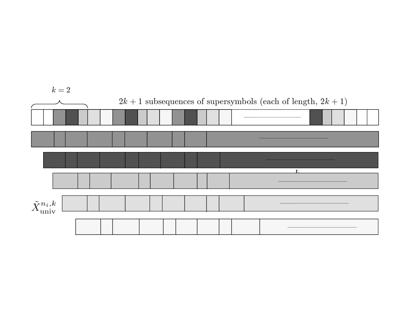
The scheme we propose is pictorially depicted in Fig. 2 below.
Refer to caption
Fig. 2: Schematic representation of the 2​k+12k+1-length sliding window denoiser

The necessity for independence of the symbols in the density estimation procedure discussed in section III-A coupled with the memoryless nature of the channel is the motivation for partitioning the problem into subsequences that are processed similarly, but separately. A 2​k+12k+1-tuple super-symbol is formed by jumping a length of 2​k+12k+1 to achieve the independence condition between the successive super-symbols. Note that there are 2​k+12k+1 such subsequences and each subsequence, ii (counting in the order of symbols in the sequence), consists of ⌈n−2​k−i−12​k+1⌉\lceil\frac{n-2k-i-1}{2k+1}\rceil, 2​k+12k+1-tuple super symbols. We label the subsequences as xnix^{n_{i}}, for 1≤i≤2​k+11\leq i\leq 2k+1. For a fixed nn, each subsequence xnix^{n_{i}} has the following super symbols,

xni={xi2​k+i,x2​k+1+i4​k+1+i,⋯,x(⌈n−2​k−1−i2​k+1⌉−1)​(2​k+1)+i(⌈n−2​k−1−i2​k+1⌉−1)​(2​k+1)+i+2​k}x^{n_{i}}=\left\{x_{i}^{2k+i},x_{2k+1+i}^{4k+1+i},\cdots,x_{\left(\lceil\frac{n-2k-1-i}{2k+1}\rceil-1\right)\left(2k+1\right)+i}^{\left(\lceil\frac{n-2k-1-i}{2k+1}\rceil-1\right)\left(2k+1\right)+i+2k}\right\}

This facilitates the extension of the ideas from the symbols of the symbol-by-symbol denoiser to the super-symbol of the 2​k+12k+1 sliding window denoiser. Some definitions are in order before we set to investigate the optimality results of the scheme. As in the symbol-by-symbol scheme, let fYn,kf_{Y}^{n,k} denote the kthk^{\text{th}} order density estimate of the noisy sequence of symbols and is computed exactly as in (24) except y,Yi∈ℝ2​k+1y,Y_{i}\in\mathbb{R}^{2k+1}. Denote ℱ[a,b],k\mathcal{F}^{[a,b],k} to be the set of all probability distribution functions with support contained in the hypercube [a,b]2​k+1[a,b]^{2k+1}. Let Dk​(xn)D_{k}(x^{n}) denote the kthk^{\text{th}}-order sliding window minimum loss and is defined as

Dk​(xn)=ming⁡E⁡[1n−2​k​∑i=k+1n−kΛ⁡(xi,g⁡(Yi−ki+k))]D_{k}(x^{n})=\min_{g}E\left[\frac{1}{n-2k}\sum_{i=k+1}^{n-k}\Lambda(x_{i},g(Y_{i-k}^{i+k}))\right] (44)

Note the similar definition of symbol-by-symbol denoisability in (7). As before, Dk​(xn)D_{k}(x^{n}) can be expressed as

Dk​(xn)=ming⁡EFxnk⊗𝒞​Λ​(X,g⁡(Y−kk))D_{k}(x^{n})=\min_{g}E_{F^{k}_{x^{n}}\otimes\mathcal{C}}\Lambda(X,g(Y_{-k}^{k})) (45)

where FxnkF^{k}_{x^{n}} is the kthk^{\text{th}} order empirical distribution of the source. Define further the sliding window denoisability of the individual sequence 𝐱=(x1,x2,x3,⋯)\mathbf{x}=\left(x_{1},x_{2},x_{3},\cdots\right) by

D⁡(𝐱)=limk→∞lim supn→∞Dk​(xn)D\left(\mathbf{x}\right)=\lim_{k\rightarrow\infty}\limsup_{n\rightarrow\infty}D_{k}(x^{n}) (46)

where the limit exists by monotonicity. In words, D⁡(𝐱)D(\mathbf{x}) is the loss of a genie who knows the underlying clean sequence and can choose to denoise with the best sliding window scheme, of arbitrary order. Extending the definition of kthk^{\text{th}}-order minimum loss to a subsequence, xnix^{n_{i}} as

Dk​(xni)=ming⁡EFxnik⊗𝒞​Λ​(X,g⁡(Y−kk))D_{k}(x^{n_{i}})=\min_{g}E_{F^{k}_{x^{n_{i}}}\otimes\mathcal{C}}\Lambda(X,g(Y_{-k}^{k})) (47)

The mapping to the corresponding kthk^{\text{th}} order input empirical distribution is given by

F^xnk​[Yn]=arg⁡minF∈ℱn[a,b]k⁡d⁡(fYn,k,∫∏i=−kkfY|xi​dF​(x−kk)⏟[F⊗𝒞]Yk)\hat{F}_{x^{n}}^{k}[Y^{n}]=\arg\min_{F\in\mathcal{F}^{[a,b]^{k}}_{n}}d\left(f_{Y}^{n,k},\underbrace{\int\prod_{i=-k}^{k}f_{Y|x_{i}}dF(x_{-k}^{k})}_{[F\otimes\mathcal{C}]_{Y}^{k}}\right) (48)

where ℱn[a,b],k⊆ℱ[a,b],k\mathcal{F}_{n}^{[a,b],k}\subseteq\mathcal{F}^{[a,b],k} denotes the set of kthk^{\text{th}} order (1≤k≤⌊n2⌋1\leq k\leq\lfloor\frac{n}{2}\rfloor) empirical distributions induced by nn-tuples with [a,b]2​k+1[a,b]^{2k+1}-valued components. P^xnδ,Δ,k\hat{P}_{x^{n}}^{\delta,\Delta,k} denotes the kk-th order estimate of the input empirical distribution of the source analogously defined as in the symbol-by-symbol case. The 2​k+12k+1-length sliding window denoiser for each of the subsequences, ii, is given by

X~ni,δ,Δ,k[yn](j)=gopt[P^xniδ,Δ,k[yni]](yj−kj+k),j∈{k+i,3k+1+i,⋯⌈n−2​k−i−12​k+1⌉}\tilde{X}^{n_{i},\delta,\Delta,k}[y^{n}](j)=g_{\text{opt}}\left[\hat{P}^{\delta,\Delta,k}_{x^{n_{i}}}[y^{n_{i}}]\right]\left(y_{j-k}^{j+k}\right),\quad j\in\left\{k+i,3k+1+i,\cdots\lceil\frac{n-2k-i-1}{2k+1}\rceil\right\} (49)

where the kthk^{\text{th}} order equivalent of the denoiser in (22) is given by

gopt​[P]​(y−kk)=arg⁡minx^∈𝒜​Λ​(⋅,x^)T​[P⊗𝒞]U|y−kk=argminx^∈𝒜∑a^∈𝒜Λ(a,x^)⋅{∑u−kk∈𝒜2​k+1:u0=a[∏i=−kkfY|x=ui(yi)P(U−kk=u−kk)]}g_{\text{opt}}[P]\left(y_{-k}^{k}\right)=\arg\min_{\hat{x}\in\mathcal{A}}\Lambda(\cdot,\hat{x})^{T}[P\otimes\mathcal{C}]_{U|y_{-k}^{k}}\\ =\arg\min_{\hat{x}\in\mathcal{A}}\sum_{\hat{a}\in\mathcal{A}}\Lambda\left(a,\hat{x}\right)\cdot\left\{\sum_{u_{-k}^{k}\in\mathcal{A}^{2k+1}:u_{0}=a}\left[\prod_{i=-k}^{k}f_{Y|x=u_{i}}(y_{i})P\left(U_{-k}^{k}=u_{-k}^{k}\right)\right]\right\} (50)

Let, ℱδ,Δk\mathcal{F}^{k}_{\delta,\Delta} denote the set of 2​k+12k+1- dimensional vectors with components in [0,1] that are integers multiples of δ\delta. Note that, P^xniδ,Δ​[zni]∈ℱδ,Δk\hat{P}_{x^{n_{i}}}^{\delta,\Delta}[z^{n_{i}}]\in\mathcal{F}_{\delta,\Delta}^{k} for all znz^{n}. Finally, let 𝒢δ,Δk={go​p​t​[P]}P∈ℱδ,Δk\mathcal{G}_{\delta,\Delta}^{k}=\{g_{opt}[P]\}_{P\in\mathcal{F}_{\delta,\Delta}^{k}} and

X~n,δ,Δ,k={X~ni,δ,Δ,k}1≤i≤2​k+1\tilde{X}^{n,\delta,\Delta,k}=\{\tilde{X}^{n_{i},\delta,\Delta,k}\}_{1\leq i\leq 2k+1} (51)

be our candidate for the nn-block 2​k+12k+1-length sliding window denoiser. It is the sequence of 2​k+12k+1 denoisers that operate individually on each of the subsequences. The cumulative loss incurred by this sequence of denoisers is defined as

LX~n,δ,Δ,k=12​k+1​∑i=12​k+1LX~ni,δ,Δ,kL_{\tilde{X}^{n,\delta,\Delta,k}}=\frac{1}{2k+1}\sum_{i=1}^{2k+1}L_{\tilde{X}^{n_{i},\delta,\Delta,k}} (52)

where, LX~ni,δ,Δ,kL_{\tilde{X}^{n_{i},\delta,\Delta,k}} is the cumulative loss incurred by the proposed denoiser for the ithi^{\text{th}}- subsequence. The following Lemma illustrates a rather intuitive fact, the average minimum kthk^{\text{th}} order sliding window loss incurred by operating on each of the subsequences is at most the minimum kthk^{\text{th}} order sliding window loss for the entire sequence.

Lemma 3

For all n≥1n\geq 1, k≤⌊n2⌋k\leq\lfloor\frac{n}{2}\rfloor,

12​k+2​Dk​(xni)≤Dk​(xn)\frac{1}{2k+2}D_{k}(x^{n_{i}})\leq D_{k}(x^{n}) (53)

V-B Performance guarantees

In this section we present Theorem 7, wherein we demonstrate that, provided certain growth constraints on the context length kk, quantization step sizes δ\delta, Δ\Delta and width of the kernel density estimate hh are satisfied, the cumulative loss, LX~n,δ,Δ,kL_{\tilde{X}^{n,\delta,\Delta,k}}, incurred by the proposed denoiser asymptotically approaches the sliding window denoisability. The growth constraints are specified at the end of this section. They are dictated by an exponential bound on the deviation between the cumulative loss, LX~n,δ,k,ΔL_{\tilde{X}^{n,\delta,k,\Delta}} and DkD_{k} which we now develop.
Let

αn​(ϵ,k,δ,Δ,ρ,γ)=[1δ+1]Δ2​k+1⋅[A(k,ϵ+δΛmax,Λmax)exp(−(n+1)G(k,ϵ+δΛmax,Λmax))+A(k,1−ρ,2γ)exp(−(n+1)G(k,1−ρ,2γ))]+e−(1−ρ)​(n−2​k)​γ22​(2​k+1)\alpha_{n}\left(\epsilon,k,\delta,\Delta,\rho,\gamma\right)=\\ \left[\frac{1}{\delta}+1\right]^{{\Delta}^{2k+1}}\cdot\left[A\left(k,\epsilon+\delta\Lambda_{\max},\Lambda_{\max}\right)\exp\left(-(n+1)G\left(k,\epsilon+\delta\Lambda_{\max},\Lambda_{\max}\right)\right)+\right.\\ \left.A\left(k,\sqrt{1-\rho},\frac{2}{\gamma}\right)\exp\left(-(n+1)G\left(k,\sqrt{1-\rho},\frac{2}{\gamma}\right)\right)\right]+e^{-(1-\rho)\frac{(n-2k)\gamma^{2}}{2(2k+1)}} (54)

where,

A⁡(k,ϵ,B)=(2​k+1)​exp⁡(2​ϵ2B2)\displaystyle A\left(k,\epsilon,B\right)=(2k+1)\exp\left(\frac{2\epsilon^{2}}{B^{2}}\right) (55)
G⁡(k,ϵ,B)=2​ϵ2(2​k+1)​B2\displaystyle G\left(k,\epsilon,B\right)=\frac{2\epsilon^{2}}{(2k+1)B^{2}} (56)

and

ν⁡(ε,δ,Δ,Λ,𝒞,k)=3​ϵ+5​δ​Λmax+4​ξΔ2​k+1​Λmax+4​λ​(Δ)​(1+ξΔ2​k+1)\nu\left(\varepsilon,\delta,\Delta,\Lambda,\mathcal{C},k\right)=3\epsilon+5\delta\Lambda_{\max}+4\xi_{\Delta}^{2k+1}\Lambda_{\max}+4\lambda(\Delta)\left(1+\xi_{\Delta}^{2k+1}\right) (57)

We now state the analogue of Theorem 4 in the present setting, which bounds the deviation of the cumulative loss incurred by the proposed 2​k+12k+1-length sliding window denoiser from the minimum possible Dk​(xn)D_{k}\left(x^{n}\right). Note that here, x∈[a,b]2​k+1x\in[a,b]^{2k+1} and Y∈[a,b]2​k+1Y\in[a,b]^{2k+1} ( 2​k+12k+1-tuple super-symbols) is the continuous valued output of the memoryless channel.

Theorem 6

For all n≥1n\geq 1, ϵ>0\epsilon>0, δ>0\delta>0, ρ=ρ⁡(ϵ,δ)\rho=\rho(\epsilon,\delta) defined in (37), Δ>0\Delta>0, 1≤k≤⌊n2⌋1\leq k\leq\lfloor\frac{n}{2}\rfloor and xn∈[a,b]nx^{n}\in[a,b]^{n}

Pr⁡(LX~n,δ,Δ,k​(xn,Yn)−Dk​(xn)>ν⁡(ε,δ,Δ,Λ,𝒞,k))≤αn​(ϵ,k,δ,Δ,ρ,γk)​∀n​ s.t ​n​hnk>nk​(𝒞,ρ,δ,K)\Pr\left(L_{\tilde{X}^{n,\delta,\Delta,k}}(x^{n},Y^{n})-D_{k}(x^{n})>\nu\left(\varepsilon,\delta,\Delta,\Lambda,\mathcal{C},k\right)\right)\leq\alpha_{n}\left(\epsilon,k,\delta,\Delta,\rho,\gamma_{k}\right)\;\forall\;n\mbox{ s.t }nh_{n}^{k}>n_{k}\left(\mathcal{C},\rho,\delta,K\right) (58)

where,

γk=ϵ(∥Λ∥L+Λmax∥Ξ∥Lk+(b−a)∥Λ∥L∥Ξ∥Lk+Λmax)\gamma_{k}=\frac{\epsilon}{\left(\parallel\Lambda\parallel_{L}+\Lambda_{\max}\parallel\Xi\parallel_{L}^{k}+(b-a)\parallel\Lambda\parallel_{L}\parallel\Xi\parallel_{L}^{k}+\Lambda_{\max}\right)} (59)

‖Ξ‖Lk\|\Xi\|_{L}^{k} (the kthk^{\text{th}} order equivalent of ‖Ξ‖L\|\Xi\|_{L} in (39)) and nk​(𝒞,ρ,δ,K)n_{k}\left(\mathcal{C},\rho,\delta,K\right) are defined in (162) and (113) respectively.

Take now, k=knk=k_{n}, δ=δn\delta=\delta_{n} and Δ=Δn\Delta=\Delta_{n} such that kn→∞k_{n}\rightarrow\infty, δn↓0\delta_{n}\downarrow 0, Δn↓0\Delta_{n}\downarrow 0,

∑n=1∞αn​(ϵ,kn,δn,Δn,ρ,γkn)<∞\sum_{n=1}^{\infty}\alpha_{n}\left(\epsilon,k_{n},\delta_{n},\Delta_{n},\rho,\gamma_{k_{n}}\right)<\infty

and nk​(𝒞,ρ,δ,K)<∞n_{k}\left(\mathcal{C},\rho,\delta,K\right)<\infty. With growth rates that satisfy these conditions let,

X^univn=X~n,δn,Δn,kn\hat{X}_{\text{univ}}^{n}=\tilde{X}^{n,\delta_{n},\Delta_{n},k_{n}} (60)

For example, it can be verified that unbounded increasing kn=log⁡(log⁡(n))k_{n}=\log\left(\log(n)\right), hn=1log⁡(n)h_{n}=\frac{1}{\log(n)}, δn​kn→0\delta_{n}k_{n}\rightarrow 0, (δn,Δn=1log⁡(n))\left(\delta_{n},\Delta_{n}=\frac{1}{\log(n)}\right) satisfies the requirements for a family, 𝒞\mathcal{C}, that has δΔn2​kn+1→0\delta_{\Delta_{n}}^{2k_{n}+1}\rightarrow 0 and loss functions that have λ⁡(Δn)​δΔn2​kn+1→0\lambda\left(\Delta_{n}\right)\delta_{\Delta_{n}}^{2k_{n}+1}\rightarrow 0. Particularly for additive Gaussian noise channels of finite variance, squared and absolute loss functions with the aforementioned growth rates of knk_{n}, Δn\Delta_{n}, δn\delta_{n} satisfy the conditions of λ⁡(Δn)​δΔn2​kn+1→0\lambda\left(\Delta_{n}\right)\delta_{\Delta_{n}}^{2k_{n}+1}\rightarrow 0 and δΔn2​kn+1→0\delta_{\Delta_{n}}^{2k_{n}+1}\rightarrow 0.
We now have the following result as a direct consequence of Theorem 6 and the Borel-Cantelli Lemma.

Theorem 7

For all 𝐱∈[a,b]∞\mathbf{x}\in[a,b]^{\infty}

limn→∞[LX^univn​(xn,Yn)−Dkn​(xn)]=0a.s.\lim_{n\rightarrow\infty}\left[L_{\hat{X}^{n}_{\text{univ}}}(x^{n},Y^{n})-D_{k_{n}}(x^{n})\right]=0\qquad a.s. (61)

In fact, we can go a step further and show that the lim sup\limsup of the cumulative loss incurred by the proposed denoiser is bounded by the sliding window denoisability. Specifically,

Corollary 1

For all 𝐱∈[a,b]∞\mathbf{x}\in[a,b]^{\infty}

lim supn→∞[LX^univn​(xn,Yn)−D⁡(𝐱)]≤0a.s.\limsup_{n\rightarrow\infty}\left[L_{\hat{X}^{n}_{\text{univ}}}(x^{n},Y^{n})-D(\mathbf{x})\right]\leq 0\qquad a.s. (62)

which is a corollary of Theorem 7, proved similarly as corollary 1 in [5].

V-C Computation complexity of the proposed denoiser

Let us summarize the computational complexity of the proposed denoisers: the “symbol-by-symbol” and the kthk^{\text{th}} order extensions. For the symbol by-symbol denoiser, we have already covered the analysis in Sections III-D1, III-D2. For XunivnX_{\text{univ}}^{n} defined in (60), we have:

Symbol-by-symbol scheme
  1. 1.

    Fast Kernel Density Estimation, O⁡(n)O(n)
    Using the techniques of fast kernel density estimation in [29], [28], [23], [14] it was shown that the complexity can be reduced from O⁡(n2)O(n^{2}) to O⁡(n)O(n).

  2. 2.

    Channel Inversion, O⁡(n3)O\left(n^{3}\right)
    The polynomial complexity of the simplex approach in linear programming problems is discussed in detail in [2].

kthk^{\text{th}} order sliding window scheme
  1. 1.

    Fast Kernel Density Estimation, O⁡(n)O\left(n\right)
    As before, the complexity of the denoiser continues to be linear in the length of the data, nn and the context length, kk, i.e., O⁡(n​kγ)​γ>0O\left(nk^{\gamma}\right)\;\gamma>0 [14].

  2. 2.

    Channel Inversion, O⁡(n6​k)O\left(n^{6k}\right)
    From the fact that the dimensionality of the contexts is length 2​k2k, the channel inversion now increases in complexity exponentially and is given by O⁡(n6​k)O\left(n^{6k}\right). Thus, our schemes are practical for small values of kk, but become unrealistic to implement as kk grows.

    This lead to our follow up work in [33] that uses quantized contexts in conjunction with the (low complexity) symbol-by-symbol denoiser that asymptotically (with increasing levels of quantization of the contexts) achieves the performance of the sequence of denoisers proposed here.

VI Universality in the stochastic setting

Our results also imply optimality for the stochastic setting when the source (clean signal) is a stationary stochastic process with distribution F𝐗F_{\mathbf{X}}. For the pair (F𝐗,𝒞)\left(F_{\mathbf{X}},\mathcal{C}\right), define the denoisability, 𝔻⁡(F𝐗,𝒞)\mathbb{D}(F_{\mathbf{X}},\mathcal{C}), as

𝔻⁡(F𝐗,𝒞)=limn→∞minX^n⁡E​LX^n​(Xn,Yn),\mathbb{D}(F_{\mathbf{X}},\mathcal{C})=\lim_{n\rightarrow\infty}\min_{\hat{X}^{n}}EL_{\hat{X}^{n}}\left(X^{n},Y^{n}\right), (63)

where the expectation is assuming XnX^{n} are the first nn symbols emitted by a source with distribution F𝐗F_{\mathbf{X}} and YnY^{n} is, as before, the nn-tuple of output noisy symbols from the channel 𝒞\mathcal{C} that corrupts XnX^{n}. This is achieved by a “genie” that has access to the true distribution, F𝐗F_{\mathbf{X}}, of the underlying clean signal, 𝐗\mathbf{X}. It has been shown in [36, 5] that the limit in (63) exists and hence the denoisability, 𝔻⁡(F𝐗,𝒞)\mathbb{D}(F_{\mathbf{X}},\mathcal{C}), is well-defined for every stationary F𝐗F_{\mathbf{X}}.

We now state the main result for the stochastic setting wherein we establish that for any stationary underlying clean sequence 𝐗∼F𝐗\mathbf{X}\sim F_{\mathbf{X}}, the expected cumulative loss incurred by our proposed scheme asymptotically achieves the denoisability, 𝔻⁡(F𝐗,𝒞)\mathbb{D}\left(F_{\mathbf{X}},\mathcal{C}\right).

Theorem 8

For all stationary 𝐗\mathbf{X}

limn→∞E​LX^univn​(Xn,Yn)=𝔻⁡(F𝐗,𝒞)\lim_{n\rightarrow\infty}EL_{\hat{X}_{\text{univ}}^{n}}\left(X^{n},Y^{n}\right)=\mathbb{D}\left(F_{\mathbf{X}},\mathcal{C}\right) (64)

If 𝐗\mathbf{X} is also ergodic then

lim supn→∞LX^univn​(Xn,Yn)=𝔻⁡(F𝐗,𝒞)​a.s.\limsup_{n\rightarrow\infty}L_{\hat{X}^{n}_{\text{univ}}}\left(X^{n},Y^{n}\right)=\mathbb{D}\left(F_{\mathbf{X}},\mathcal{C}\right)\;a.s. (65)

Given the results established for the semi-stochastic setting, the proof is analogous to that of Theorem 3 in [5] except for some subtle differences in our setting due to the continuous input and output alphabets. We, however, do provide the proof of the above statement for completeness and for accommodating these differences in Appendix H.

We conclude this section by comparing the proposed sequence of denoisers to the DUDE-like schemes in [5] for the case of finite input (or underlying clean data) and continuous valued output (noisy data) . By a minor modification, the proposed denoiser collapses to that in [5] when, as in the setting onf [5], the channel input alphabet is finite. This is illustrated by comparing the first pass of the DUDE-like denoiser with a modified version of the proposed scheme through the schematic representation in Fig. 3. The theoretical details of the equivalence of the modification shown in Fig. 3 below to the denoiser in [5] are elaborated in Appendix I.

Refer to caption
Fig. 3: Modification to our proposed scheme that is equivalent to that in [5]

VII Experimental Results

In this section, we discuss experimental results of applying the proposed scheme to denoising 256-level gray scale images. We demonstrate efficacy of the scheme with results of its application to cases of additive and multiplicative Gaussian noise. In addition, we consider a highly nonlinear, non-conventional noise distribution: a locally varying Rayleigh noise whose variance is a function of the gray level of the underlying clean image. The first pass of the denoiser is performed using a Fast Kernel Density Estimation approach proposed in [15] and a channel inversion procedure. This channel inversion is performed using a convex optimization linear programming technique that maps the output kthk^{\text{th}}-order density estimate to the corresponding input kthk^{\text{th}}-order input empirical distribution in accordance with (48). The experimental results presented in this section have been obtained by implementing the scheme of the previous sections, with no heuristic modifications that are likely to boost the performance. The practical implementation aspects are discussed in greater detail and depth in [32], [33].

The first example we consider is, denoising of the boats image that is corrupted by an additive white noise channel (AWGN) with, σ=20\sigma=20. The loss function, Λ\Lambda, to be minimized in this case is the squared error between the true clean image and our denoised estimate. The denoiser in this case is a mapping from ℝ→𝒜={0,⋯255}\mathbb{R}\rightarrow\mathcal{A}=\{0,\cdots 255\} and reduces to that in (50). Results of the proposed denoising scheme are shown in the Fig.  5 below with context length, kk, ranging from 1 to 6. The context (for k>1k>1) around any location, ii, in the block of noisy data are 2D neighborhoods. The 2D contexts for various values of kk are shown in Fig. 4 below. As is evident from both, the reported Root Mean Squared Error (RMSE) figures and the perceptual quality, we are able to achieve improved denoising performance with increasing context lengths. Finally, we compare the results of the proposed scheme to that achieved by wavelet-based thresholding scheme [9] and Bayesian Least Squares Gaussian Scaled Mixture (BLS-GSM) denoiser in [26]. Increasing context lengths, kk, translates to accruing increasing kthk^{\text{th}}-order statistics from the finite block length data. This is the classic trade-off between increasing context lengths and reliability of the associated higher order statistics is seen in Fig.  6 where we see only marginal gains in the RMSE between, k=4k=4 and k=6k=6. The results for the AWGN case are primarily aimed at demonstrating the practicality of the proposed scheme fully acknowledging the performance lead of schemes like the BLS-GSM that are particularly catered to the problem of denoising in the case of AWGN channels. The benefits of the proposed approach are in fact highlighted in unconventional cases like nonlinear noise channels which will be discussed next.

Refer to caption
Fig. 4: 2D Contexts for context length, kk
     Refer to caption Refer to caption
     Refer to caption Refer to caption
     RMSE = 14.7354 RMSE = 13.0945
     Refer to caption Refer to caption
     RMSE = 11.2899 RMSE = 11.2610
     Refer to caption Refer to caption
     RMSE = 11.1782 RMSE = 7.842
Fig. 5: Row 1- left: Original image, right: Noisy image, σ=20\sigma=20; Denoised Images using, Row 2- left: k=1k=1 right: k=2k=2; Row 3- left: k=4k=4, right: k=6k=6; Row 4- left: the scheme in [9], right: the scheme in [26]
Refer to caption
Fig. 6: Comparison of RMSE of the denoised image for various context lengths, kk

Another example of the application of the proposed scheme is in denoising an image corrupted with an unconventional distribution as discussed earlier in this section. More specifically, we simulate the noisy image by using a gray-level dependent Rayleigh distribution (with probability density function, OPENf⁡(x)=xb2​e−x22​b2)f(x)=\frac{x}{b^{2}}e^{\frac{-x^{2}}{2b^{2}}}) whose variance parameter, BB, is chosen as a function of clean image’s gray level at that location. In this particular example, we generate a matrix of 256x256 Rayleigh distributed random variables whose parameters BB are chosen according to the following rule, B⁡(i,j)=I⁡(i,j)∗35/256B(i,j)=I(i,j)*35/256, where I⁡(i,j)I(i,j) is the true value of the clean image at location (i,j)(i,j). We will discuss the denoising performance only in the symbol-by-symbol case in this setting in favor of succinctness to convey the point of efficacy of the proposed scheme. More detailed results and discussions on this problem setting can be found in [32]. We compare, in Fig. 7, the empirical distribution estimate, F^xn\hat{F}_{x^{n}}, of the underlying clean image with the histogram generated from access to the “true” clean image. We also compare these results to the smoothed histogram estimate of the true clean image that was produced using the Kernel Density estimation approach in [15]. From a visual inspection of the figure, it is evident that we are able to reasonably recover the true marginal empirical distribution of the underlying clean image and correspondingly the estimate of the true image.

Refer to caption Refer to caption
RMSEnoise\text{RMSE}_{\text{noise}} = 38.802
Refer to caption Refer to caption
RMSE = 11.2839
Fig. 7: Row 1- left: Original image, right: Noisy image; Denoised images using Row 2- left: symbol-symbol scheme, right: Comparison of Distribution estimates for the symbol-by-symbol denoiser

Finally, we present the results of denoising the boats image that is corrupted by a multiplicative Gaussian noise with a distribution, 𝒩⁡(1,0.2)\mathcal{N}(1,0.2) in Fig. 8. The noise in this case literally multiplies this case literally multiplies the original clean image to corrupt it and as such, the effects are relatively more catastrophic. We compare, qualitatively, the results from the proposed denoiser with that of [26] to validate its efficacy.

Refer to caption Refer to caption
Fig. 8: Row 1- left: Original image, right: Noisy image; Denoised images using Row 2- left: proposed scheme, right: BLS-GSM [26]

VIII Conclusion and Future Directions

We have presented a family of schemes for denoising continuous amplitude signals that is universally optimal. A salient feature of our setting and results is the wide generality of channels and loss functions for which they apply. The techniques presented in this paper draw from the “DUDE framework” in [36]. A weighted ‘context aggregation’ was suggested in [36] as an approach to enhance the performance of the DUDE in the first pass of the statistics collection. The proposed technique provides a natural context aggregation mechanism whereby neighboring contexts in addition to the observed are weighted by the kernel in the density estimation step. The denoiser proposed in [5] was shown to be asymptotically universal and extended the domain of applicability of DUDE-like schemes to cases where the noise is continuous valued. This approach, even though elegant theoretically, suffers from some of the same issues as the DUDE in terms of sparseness of statistics for large alphabet sizes. Our technique addresses this problem for the problem setting considered in [5] by natural context aggregation induced by the kernel density estimation. In the setting where the underlying clean signal is discrete-valued, taking values in a finite alphabet space, a slight modification of our scheme has been shown to reduce to the scheme in [5]. We also simultaneously provide a framework to address the case of continuous valued alphabets, where there is need to learn distribution functions instead of individual mass points as in the discrete-valued case. Finally, the proposed scheme is practical and tractable in its computational requirements as demonstrated by the experimental results.

The experimental results in this paper seem promising enough to motivate further exploration of practical aspects of the proposed scheme. This is an interesting future direction that is currently under investigation. Additional directions of research include studying the applicability of recursive density estimation techniques discussed in [18] in designing recursive denoisers as an alternative to the scheme presented in this paper. This would be particularly useful in multidimensional data applications like denoising noise corrupted video. It could also be of theoretical interest to understand the implications of a recursive structure to the denoiser and its associated optimality results.

Appendix A Conditions on the channel

In addition to conditions C1-C4 in section II, the following conditions on the channel (noise distribution) round up the necessary assumptions for the performance guarantees made in this work.

  • C5.

    The channel satisfies the uniform Lipschitz continuity condition,

    supy∈ℝ‖fY|x​(y)‖B​L<∞\sup_{y\in\mathbb{R}}\|f_{Y|x}(y)\|_{BL}<\infty (66)

    where

    ‖fY|x​(y)‖B​L\displaystyle{}\|f_{Y|x}(y)\|_{BL} =\displaystyle= ‖fY|x​(y)‖L+‖fY|x​(y)‖∞\displaystyle\|f_{Y|x}(y)\|_{L}+\|f_{Y|x}(y)\|_{\infty} (67)
    ‖fY|x​(y)‖L\displaystyle\|f_{Y|x}(y)\|_{L} =\displaystyle= supx≠zx,z∈[a,b]|fY|x​(y)−fY|z​(y)||x−z|<∞,∀y∈ℝ\displaystyle\sup_{x\neq z\atop x,z\in[a,b]}\frac{\left|f_{Y|x}(y)-f_{Y|z}(y)\right|}{|x-z|}<\infty,\;\forall y\in\mathbb{R} (68)
    ‖fY|x​(y)‖∞\displaystyle\|f_{Y|x}(y)\|_{\infty} =\displaystyle= supx∈[a,b]fY|x​(y)\displaystyle\sup_{x\in[a,b]}f_{Y|x}(y) (69)
  • C6.

    The conditional densities, additionally, satisfy the following Lipschitz continuity condition,

    ∥Ξ∥L=sup0<Δ<(b−a)ξΔΔ<∞\parallel\Xi\parallel_{L}=\sup_{0<\Delta<(b-a)}\frac{\xi_{\Delta}}{\Delta}<\infty (70)

    where, ξΔ\xi_{\Delta} is defined in (38).

  • C7a.

    The family of conditional densities, 𝒞\mathcal{C}, have uniformly bounded second order universal derivatives, i.e., ∃\exists a ℬ𝒞\mathcal{B}_{\mathcal{C}} s.t. 0<ℬ𝒞<∞0<\mathcal{B}_{\mathcal{C}}<\infty and D2∗​(fY|x)<ℬ𝒞,∀x∈[a,b]D_{2}^{\ast}\left(f_{Y|x}\right)<\mathcal{B}_{\mathcal{C}},\forall x\in[a,b], where the second order universal derivative is defined as (refer [6] for further details)

    D2∗​(fY|x)=lim infh↓0∫|(fY|x∗ϕh)(2)|​𝑑yD_{2}^{\ast}\left(f_{Y|x}\right)=\liminf_{h\downarrow 0}\int\left|\left(f_{Y|x}\ast\phi_{h}\right)^{(2)}\right|dy (71)

    ϕh​(x)=1h​ϕ​(xh)\phi_{h}(x)=\frac{1}{h}\phi\left(\frac{x}{h}\right), ϕ∈C∞\phi\in C^{\infty}, C∞C^{\infty} is a set of functions that have infinitely many continuous derivatives with compact support and f(s)f^{(s)} denotes the ss-th derivative of ff. This is a mild technical condition that enables the proof of the convergence of marginal density estimates at the output of the memoryless channel to the true marginal density. Note that we are not imposing the differentiability of the conditional densities of the channel themselves. We are, instead, proposing a milder constraint that the smoothed version of the channel conditional densities is “differentiable enough”. This condition is trivially satisfied if we have a family of conditional densities that have a uniformly absolutely continuous derivative.

  • C7b.

    An alternative to the previous condition on the family of conditional densities of the channel is, lim|t|→0Ω𝒞​(t)=0\lim_{|t|\rightarrow 0}\Omega_{\mathcal{C}}(t)=0, where

    Ω𝒞​(t)=supx∈[a,b]ωx​(t)\displaystyle{}\Omega_{\mathcal{C}}(t)=\sup_{x\in[a,b]}\omega_{x}(t) (72)

    and

    ωx​(t)=∫|fY|x​(y−t)−fY|x​(y)|​𝑑y\displaystyle{}\omega_{x}(t)=\int\left|f_{Y|x}(y-t)-f_{Y|x}(y)\right|dy (73)

    From the fact [37] that, for any f∈L1​(ℝ)f\in L_{1}(\mathbb{R}), the corresponding, L1L_{1}-modulus of continuity,

    ω⁡(t)=∫|f⁡(x−t)−f⁡(x)|​𝑑x→0,as|t|→0\omega(t)=\int\left|f(x-t)-f(x)\right|dx\rightarrow 0,\;\text{as}\;|t|\rightarrow 0

    and

    ‖ω‖∞≤2​‖f‖1<∞\|\omega\|_{\infty}\leq 2\|f\|_{1}<\infty

    it follows that the global L1L_{1}-modulus of continuity, Ω𝒞​(t)\Omega_{\mathcal{C}}(t), is well-defined for all tt and families of conditional densities, 𝒞\mathcal{C}. In other words, this condition demands uniform convergence of the L1L_{1}-moduli of continuity of the individual members comprising the family of conditional densities.

Appendix B Proof of Lemma 26

A theorem necessary for the proof of Lemma 26 is as follows

Theorem 9

Every kernel KK with ∫K=1,K≥0\int K=1,K\geq 0 is an approximate identity, i.e for limn→∞hn=0\lim_{n\rightarrow\infty}h_{n}=0 and every fi∈L1f_{i}\in L_{1}, s.t. D2∗​(fi)<∞D_{2}^{\ast}\left(f_{i}\right)<\infty are uniformly bounded we have

limn→∞∫|(1n​∑i=1nfi)∗Khn−(1n​∑i=1nfi)|=0\lim_{n\rightarrow\infty}\int\left|\left(\frac{1}{n}\sum_{i=1}^{n}f_{i}\right)\ast K_{h_{n}}-\left(\frac{1}{n}\sum_{i=1}^{n}f_{i}\right)\right|=0

An alternate formulation of the approximation identity is the following,

Theorem 10

Every kernel KK with ∫K=1,K≥0\int K=1,K\geq 0 is an approximate identity, i.e for limn→∞hn=0\lim_{n\rightarrow\infty}h_{n}=0 and every fi∈L1f_{i}\in L_{1}, s.t. lim|t|→0Ω𝒞​(t)=0\lim_{|t|\rightarrow 0}\Omega_{\mathcal{C}}(t)=0

limn→∞∫|(1n​∑i=1nfi)∗Khn−(1n​∑i=1nfi)|=0\lim_{n\rightarrow\infty}\int\left|\left(\frac{1}{n}\sum_{i=1}^{n}f_{i}\right)\ast K_{h_{n}}-\left(\frac{1}{n}\sum_{i=1}^{n}f_{i}\right)\right|=0

A definition regarding the notion of an associated kernel, LL, with the kernel, KK that is necessary for the subsequent proof is,

Definition 5

The function LL defined by

L⁡(x)\displaystyle L(x) =\displaystyle= (−1)s​∫x∞(y−x)s−1(s−1)!​K​(y)​𝑑y(x>0)\displaystyle(-1)^{s}\int_{x}^{\infty}\frac{(y-x)^{s-1}}{(s-1)!}K(y)dy\qquad(x>0)
L⁡(−x)\displaystyle L(-x) =\displaystyle= (−1)s​L​(x)(x<0)\displaystyle(-1)^{s}L(x)\qquad(x<0)

is the kernel associated with kernel KK. The function LL is sometimes said to have a parameter ss since it figures in the definition of LL. When KK is symmetric, LL is symmetric.

Furthermore,

∫|L|≤1s!​∫|x|s​|K⁡(x)|​𝑑x\int|L|\leq\frac{1}{s!}\int|x|^{s}|K(x)|dx (74)

for all nonnegative integers ss. For s=0s=0, we define L=KL=K. For K≥0K\geq 0, we have the equality

∫|L|=1s!​∫|x|s​|K⁡(x)|​𝑑x\int|L|=\frac{1}{s!}\int|x|^{s}|K(x)|dx (75)

Finally,

∫L\displaystyle\int L =\displaystyle= ∫xss!​K​(x)​𝑑x\displaystyle\int\frac{x^{s}}{s!}K(x)dx
=\displaystyle= {0:s​ odd0:s​ even, and the order of ​K​ is>s\displaystyle\left\{\begin{array}[]{r@{\quad:\quad}l}0&s\mbox{ odd}\\ 0&s\mbox{ even, and the order of }K\mbox{ is}>s\end{array}\right.
Proof:

Let us start with the case that fif_{i} has s−1s-1 absolutely continuous derivatives. Then, by Taylor’s series expansion with remainder,

fi​(x+y)−fi​(x)=∑j=1s−1yjj!​fi(j)​(x)+∫xx+y(x+y−u)s−1(s−1)!​fi(s)​(u)​𝑑uf_{i}(x+y)-f_{i}(x)=\sum_{j=1}^{s-1}\frac{y^{j}}{j!}f_{i}^{(j)}(x)+\int_{x}^{x+y}\frac{(x+y-u)^{s-1}}{(s-1)!}f_{i}^{(s)}(u)du

so that, for class ss kernels KK,

(1n​∑i=1nfi)∗Khn−(1n​∑i=1nfi)\displaystyle\left(\frac{1}{n}\sum_{i=1}^{n}f_{i}\right)\ast K_{h_{n}}-\left(\frac{1}{n}\sum_{i=1}^{n}f_{i}\right) (79)
=\displaystyle= 1n​∫(∑i=1nfi​(x+y)−∑i=1nfi​(x))​Khn​(y)​𝑑y(recall that​∫K=1)\displaystyle\frac{1}{n}\int\left(\sum_{i=1}^{n}f_{i}(x+y)-\sum_{i=1}^{n}f_{i}(x)\right)K_{h_{n}}(y)dy\qquad(\mbox{recall that}\int K=1)
=\displaystyle= 1n​∑i=1n[∑j=1s−10+∫∫xx+y(x+y−u)s−1(s−1)!​fi(s)​(u)​𝑑u​Khn​(y)​𝑑y]\displaystyle\frac{1}{n}\sum_{i=1}^{n}\left[\sum_{j=1}^{s-1}0+\int\int_{x}^{x+y}\frac{(x+y-u)^{s-1}}{(s-1)!}f_{i}^{(s)}(u)du\;K_{h_{n}}(y)dy\right]
=\displaystyle= 1n∑i=1n[∫x∞fi(s)(u)∫u−x∞(x+y−u)s−1(s−1)!Khn(y)dydu\displaystyle\frac{1}{n}\sum_{i=1}^{n}\left[\int_{x}^{\infty}f_{i}^{(s)}(u)\int_{u-x}^{\infty}\frac{(x+y-u)^{s-1}}{(s-1)!}K_{h_{n}}(y)dy\;du\right.
−∫−∞xfi(s)(u)∫−∞u−x(x+y−u)s−1(s−1)!Khn(y)dydu]\displaystyle\left.-\int_{-\infty}^{x}f_{i}^{(s)}(u)\int_{-\infty}^{u-x}\frac{(x+y-u)^{s-1}}{(s-1)!}K_{h_{n}}(y)dy\;du\right]
=\displaystyle= 1n∑i=1n[∫x∞fi(s)(u)(−1)s(L)hn(u−x)du\displaystyle\frac{1}{n}\sum_{i=1}^{n}\left[\int_{x}^{\infty}f_{i}^{(s)}(u)(-1)^{s}(L)_{h_{n}}(u-x)du\right.
−∫−∞xfi(s)(u)(−1)(−1)s(−1)s(L)hn(x−u)du]\displaystyle\left.-\int_{-\infty}^{x}f_{i}^{(s)}(u)(-1)(-1)^{s}(-1)^{s}(L)_{h_{n}}(x-u)du\right]
=\displaystyle= 1n​∑i=1n[∫−∞∞fi(s)​(u)​(L)hn​(x−u)​𝑑u]\displaystyle\frac{1}{n}\sum_{i=1}^{n}\left[\int_{-\infty}^{\infty}f_{i}^{(s)}(u)\;(L)_{h_{n}}(x-u)du\right]
=\displaystyle= 1n​∑i=1nhs​fi(s)∗Lhn\displaystyle\frac{1}{n}\sum_{i=1}^{n}h^{s}f_{i}^{(s)}\ast L_{h_{n}}

where (L)hn(L)_{h_{n}} is the kernel associated with KhnK_{h_{n}} and LL is the kernel associated with KK. Therefore, by Young’s inequality [30],

∫|(1n​∑i=1nfi)∗Khn−(1n​∑i=1nfi)|=∫|1n​∑i=1nhns​fi(s)∗Lhn|\displaystyle\int\left|\left(\frac{1}{n}\sum_{i=1}^{n}f_{i}\right)\ast K_{h_{n}}-\left(\frac{1}{n}\sum_{i=1}^{n}f_{i}\right)\right|=\int\left|\frac{1}{n}\sum_{i=1}^{n}{h_{n}}^{s}f_{i}^{(s)}\ast L_{h_{n}}\right|
≤hnsn​∫|∑i=1nfi(s)|​∫|L|\displaystyle\leq\frac{h_{n}^{s}}{n}\int\left|\sum_{i=1}^{n}f_{i}^{(s)}\right|\int|L|
≤hnsn​(∑i=1n∫|fi(s)|)​∫|L|\displaystyle\leq\frac{h_{n}^{s}}{n}\left(\sum_{i=1}^{n}\int\left|f_{i}^{(s)}\right|\right)\int|L| (80)

Since fif_{i}’s have (s−1)(s-1) absolutely continuous derivatives, ∫|fi(s)|<∞\int|f_{i}^{(s)}|<\infty, and further if ∫|fi(s)|<M<∞\int|f_{i}^{(s)}|<M<\infty, ∀i\forall i (uniformly bounded) the inequality in (80) simplifies to

∫|(1n​∑i=1nfi)∗Khn−(1n​∑i=1nfi)|≤hns​M​∫|L|\displaystyle\int\left|\left(\frac{1}{n}\sum_{i=1}^{n}f_{i}\right)\ast K_{h_{n}}-\left(\frac{1}{n}\sum_{i=1}^{n}f_{i}\right)\right|\leq h_{n}^{s}M\int|L| (81)

Since,

∫|L|≤1s!​∫|x|s​|K⁡(x)|​𝑑x=BK<∞\int|L|\leq\frac{1}{s!}\int|x|^{s}|K(x)|dx=B_{K}<\infty (82)

for KK being an order s kernel, inequality in equation (81) becomes

∫|(1n​∑i=1nfi)∗Khn−(1n​∑i=1nfi)|≤hns​M​BK\displaystyle\int\left|\left(\frac{1}{n}\sum_{i=1}^{n}f_{i}\right)\ast K_{h_{n}}-\left(\frac{1}{n}\sum_{i=1}^{n}f_{i}\right)\right|\leq h_{n}^{s}MB_{K} (83)

Taking limit n→∞n\rightarrow\infty on either sides, we get

0≤limn→∞∫|(1n​∑i=1nfi)∗Khn−(1n​∑i=1nfi)|≤limn→∞hns​M​BK=0\displaystyle 0\leq\lim_{n\rightarrow\infty}\int\left|\left(\frac{1}{n}\sum_{i=1}^{n}f_{i}\right)\ast K_{h_{n}}-\left(\frac{1}{n}\sum_{i=1}^{n}f_{i}\right)\right|\leq\lim_{n\rightarrow\infty}h_{n}^{s}MB_{K}=0 (84)

This can be extended to the general fif_{i}’s using the universal derivative defined earlier. As a reminder,

Ds∗​(fi)≜lim infh↓0∫|(fi∗ϕh)(s)|D_{s}^{\ast}\left(f_{i}\right)\triangleq\liminf_{h\downarrow 0}\int\left|\left(f_{i}\ast\phi_{h}\right)^{(s)}\right| (85)

where, ϕ\phi is a mollifier.

Mollifiers are class 0 kernels, nonnegative and zero outside [−1,1][-1,1]. They also have infinitely many continuous derivatives and is called a mollifier because of its exceptional smoothing properties. An example of a mollifier is

K⁡(x)=C​e−11−x2,|x|≤1K(x)=Ce^{-\frac{1}{1-x^{2}}},\;|x|\leq 1 (86)

For a class ss kernel, KK, and a family of density functions {fi}i∈ℕ\{f_{i}\}_{i\in\mathbb{N}} with associated universal derivatives that are uniformly bounded, i.e., D2∗​(fi)<ℬ𝒞<∞D_{2}^{\ast}\left(f_{i}\right)<\mathcal{B}_{\mathcal{C}}<\infty, ∀i∈ℕ\forall i\in\mathbb{N}, it can then be shown that,

∫|(1n​∑i=1nfi)∗Khn−(1n​∑i=1nfi)|\displaystyle\int\left|\left(\frac{1}{n}\sum_{i=1}^{n}f_{i}\right)\ast K_{h_{n}}-\left(\frac{1}{n}\sum_{i=1}^{n}f_{i}\right)\right| ≤\displaystyle\leq 1n​∑i=1n∫|fi∗Khn−fi|\displaystyle\frac{1}{n}\sum_{i=1}^{n}\int\left|f_{i}\ast K_{h_{n}}-f_{i}\right| (87)
≤\displaystyle\leq 1n​∑i=1nhns​Ds∗​(fi)​∫|L|\displaystyle\frac{1}{n}\sum_{i=1}^{n}h_{n}^{s}D_{s}^{\ast}\left(f_{i}\right)\int\left|L\right|
≤\displaystyle\leq 1n​∑i=1nhns​ℬ𝒞​∫|L|\displaystyle\frac{1}{n}\sum_{i=1}^{n}h_{n}^{s}\mathcal{B}_{\mathcal{C}}\int\left|L\right|
=\displaystyle= hns​ℬ𝒞​∫|L|\displaystyle h_{n}^{s}\mathcal{B}_{\mathcal{C}}\int\left|L\right|

Taking limits on both sides we get,

limn→∞∫|(1n​∑i=1nfi)∗Khn−(1n​∑i=1nfi)|=0\displaystyle\lim_{n\rightarrow\infty}\int\left|\left(\frac{1}{n}\sum_{i=1}^{n}f_{i}\right)\ast K_{h_{n}}-\left(\frac{1}{n}\sum_{i=1}^{n}f_{i}\right)\right|=0 (88)

∎

Proof:
fi​(x)=fi​(x)​∫Kh​(t)​𝑑t=∫fi​(x)​Kh​(t)​𝑑t,∀i\displaystyle f_{i}(x)=f_{i}(x)\int K_{h}(t)dt=\int f_{i}(x)K_{h}(t)dt,\quad\forall i (89)

Therefore,

|(1n​∑i=1nfi∗Kh)​(x)−1n​∑i=1nfi​(x)|=|∫[1n​∑i=1nfi​(x−t)−1n​∑i=1nfi​(x)]​Kh​(t)​𝑑t|\displaystyle\left|\left(\frac{1}{n}\sum_{i=1}^{n}f_{i}\ast K_{h}\right)(x)-\frac{1}{n}\sum_{i=1}^{n}f_{i}(x)\right|=\left|\int\left[\frac{1}{n}\sum_{i=1}^{n}f_{i}(x-t)-\frac{1}{n}\sum_{i=1}^{n}f_{i}(x)\right]K_{h}(t)dt\right|
≤∫|1n​∑i=1nfi​(x−t)−1n​∑i=1nfi​(x)|​|Kh​(t)|1p​|Kh​(t)|1p′​𝑑t\displaystyle\leq\int\left|\frac{1}{n}\sum_{i=1}^{n}f_{i}(x-t)-\frac{1}{n}\sum_{i=1}^{n}f_{i}(x)\right|\left|K_{h}(t)\right|^{\frac{1}{p}}\left|K_{h}(t)\right|^{\frac{1}{p^{\prime}}}dt (90)

where 1p+1p′=1,(1p′=0 if p=1)\frac{1}{p}+\frac{1}{p^{\prime}}=1,\left(\frac{1}{p^{\prime}}=0\text{ if }p=1\right). Applying Holder’s inequality with exponents pp and p′p^{\prime}, and then raising both sides to the pthp^{\text{th}} power and integrating with respect to x, we obtain

∫|(1n​∑i=1nfi∗Kh)​(x)−1n​∑i=1nfi​(x)|p​𝑑x\displaystyle\int\left|\left(\frac{1}{n}\sum_{i=1}^{n}f_{i}\ast K_{h}\right)(x)-\frac{1}{n}\sum_{i=1}^{n}f_{i}(x)\right|^{p}dx
≤∫[∫|1n​∑i=1nfi​(x−t)−1n​∑i=1nfi​(x)|p​|Kh​(t)|​𝑑t]​[∫|Kh​(t)|​𝑑t]pp′​𝑑x\displaystyle\leq\int\left[\int\left|\frac{1}{n}\sum_{i=1}^{n}f_{i}(x-t)-\frac{1}{n}\sum_{i=1}^{n}f_{i}(x)\right|^{p}\left|K_{h}(t)\right|dt\right]\left[\int\left|K_{h}(t)\right|dt\right]^{\frac{p}{p^{\prime}}}dx
=|K|∫1pp′⁡[∫|1n​∑i=1nfi​(x−t)−1n​∑i=1nfi​(x)|p​|Kh​(t)|​𝑑t]​𝑑x\displaystyle=\|K\|_{1}^{\frac{p}{p^{\prime}}}\int\left[\int\left|\frac{1}{n}\sum_{i=1}^{n}f_{i}(x-t)-\frac{1}{n}\sum_{i=1}^{n}f_{i}(x)\right|^{p}\left|K_{h}(t)\right|dt\right]dx
≤|K|∫1pp′⁡[1n​∑i=1n∫|fi​(x−t)−fi​(x)|p​|Kh​(t)|​𝑑t]​𝑑x\displaystyle\leq\|K\|_{1}^{\frac{p}{p^{\prime}}}\int\left[\frac{1}{n}\sum_{i=1}^{n}\int\left|f_{i}(x-t)-f_{i}(x)\right|^{p}\left|K_{h}(t)\right|dt\right]dx (91)

Changing the order of integration in the last expression (which is justified since the integrand is nonnegative), we obtain

‖(1n​∑i=1nfi)∗Kh−1n​∑i=1nfi‖pp\displaystyle\|\left(\frac{1}{n}\sum_{i=1}^{n}f_{i}\right)\ast K_{h}-\frac{1}{n}\sum_{i=1}^{n}f_{i}\|_{p}^{p} ≤\displaystyle\leq ‖K‖1pp′​∫|Kh​(t)|​1n​∑i=1nωi​(t)​𝑑t\displaystyle\|K\|_{1}^{\frac{p}{p^{\prime}}}\int\left|K_{h}(t)\right|\frac{1}{n}\sum_{i=1}^{n}\omega_{i}(t)dt (92)
≤\displaystyle\leq ‖K‖1pp′​∫|Kh​(t)|​Ω​(t)​𝑑t\displaystyle\|K\|_{1}^{\frac{p}{p^{\prime}}}\int\left|K_{h}(t)\right|\Omega(t)dt

For δ>0\delta>0,

Ih=∫|Kh(t)|Ω(t)dt=∫|t|<δ+∫|t|≥δ=Ah,δ+Bh,δ\displaystyle I_{h}=\int\left|K_{h}(t)\right|\Omega(t)dt=\int_{|t|<\delta}+\int_{|t|\geq\delta}=A_{h,\delta}+B_{h,\delta} (93)

Since, we have Ω⁡(t)→0\Omega(t)\rightarrow 0 as |t|→0|t|\rightarrow 0, for η>0\eta>0, we can choose δ\delta so small that Ω⁡(t)<η\Omega(t)<\eta if |t|<δ|t|<\delta. Then

Ah,δ≤η​∫|t|<δ|Kh​(t)|​𝑑t≤η​‖K‖1,∀h>0\displaystyle A_{h,\delta}\leq\eta\int_{|t|<\delta}\left|K_{h}(t)\right|dt\leq\eta\|K\|_{1},\quad\forall h>0 (94)

Also, Ω\Omega is a bounded function by Minkowski’s inequality [note that ‖Ω‖∞≤supi∈ℕ‖ωi‖∞≤supi∈ℕ(2​‖fi‖p)p\|\Omega\|_{\infty}\leq\sup_{i\in\mathbb{N}}\|\omega_{i}\|_{\infty}\leq\sup_{i\in\mathbb{N}}\left(2\|f_{i}\|_{p}\right)^{p}, which for p=1p=1, becomes ‖Ω‖∞≤2\|\Omega\|_{\infty}\leq 2], so that Bh,δB_{h,\delta} is less than a constant multiple of ∫|t|≥δ|Kh​(t)|​𝑑t\int_{|t|\geq\delta}\left|K_{h}(t)\right|dt, which tends to zero with hh. This proves that Ih→0I_{h}\rightarrow 0 as h→0h\rightarrow 0 and the theorem follows. ∎

Another lemma necessary for the proof of Lemma 26 is the following.

Lemma 4

(A Multinomial distribution inequality)

Let N1,⋯,NkN_{1},\cdots,N_{k} be a multinomial random vector with parameters n,p1,⋯,pkn,p_{1},\cdots,p_{k}. Then

P⁡(∑i=1k|Nin−pi|≥ϵ)≤2k+1​e−n​ϵ22P\left(\sum_{i=1}^{k}\left|\frac{N_{i}}{n}-p_{i}\right|\geq\epsilon\right)\leq 2^{k+1}e^{\frac{-n\epsilon^{2}}{2}} (95)

Proof

By Scheffe’s theorem,

∑i=1k|Nin−pi|=2​supA|N⁡(𝔸)n−P⁡(𝔸)|\sum_{i=1}^{k}\left|\frac{N_{i}}{n}-p_{i}\right|=2\sup_{A}\left|\frac{N(\mathbb{A})}{n}-P(\mathbb{A})\right| (96)

where, 𝔸\mathbb{A} = {all 2k2^{k} possible sets of integers from 1,⋯,k1,\cdots,k} and N⁡(𝔸)N(\mathbb{A}) is the cardinality of 𝔸\mathbb{A}. By Bonferroni’s inequality and Hoeffding’s inequality,

P⁡(sup𝔸|N⁡(𝔸)n−P⁡(𝔸)|≥ϵ2)≤2k​2​e−2​n​(ϵ2)2P\left(\sup_{\mathbb{A}}\left|\frac{N(\mathbb{A})}{n}-P(\mathbb{A})\right|\geq\frac{\epsilon}{2}\right)\leq 2^{k}2e^{-2n\left(\frac{\epsilon}{2}\right)^{2}} (97)

The expected value of fn​(x)f^{n}(x) is denoted by,

gh​(x)=E⁡(fn​(x))=1n​hd​∑i=1n∫K⁡(x−yh)​fi​(y)​𝑑yg_{h}(x)=E(f^{n}(x))=\frac{1}{nh^{d}}\sum_{i=1}^{n}\int K\left(\frac{x-y}{h}\right)f_{i}(y)dy (98)
Proof:

Let ghg_{h} be defined as in (98). By Theorem 1, it is enough to show that ∫|fn​(x)−gh​(x)|​𝑑x→0\int|f^{n}(x)-g_{h}(x)|dx\rightarrow 0 exponentially. Let μn\mu_{n} be the empirical probability measure for X1,X2,⋯,XnX_{1},X_{2},\cdots,X_{n} and note that

fn​(x)=1hd​∫K⁡(x−yh)​μn​(𝑑y)\displaystyle f^{n}(x)=\frac{1}{h^{d}}\int K\left(\frac{x-y}{h}\right)\mu_{n}(dy) (99)

For given ϵ>0\epsilon>0, find finite constants M,L,N,a1,⋯,aNM,L,N,a_{1},\cdots,a_{N} and disjoint finite rectangles A1,⋯,ANA_{1},\cdots,A_{N} in ℝd\mathbb{R}^{d} such that the function

K∗​(x)=∑i=1Nai​IAi​(x)K^{\ast}(x)=\sum_{i=1}^{N}a_{i}I_{A_{i}}(x)\\ (101)

satisfies: |K∗|≤M,K∗=0|K^{\ast}|\leq M,K^{\ast}=0 outside [−L,L]d,[-L,L]^{d}, and ∫|K⁡(x)−K∗​(x)|​𝑑x<ϵ\int|K(x)-K^{\ast}(x)|dx<\epsilon. Define gh∗g_{h}^{\ast} and fn∗f^{n\ast} as ghg_{h} and fnf^{n} with K∗K^{\ast} instead of KK. Then

∫|fn​(x)−gh​(x)|​𝑑x≤∫|fn(x)−fn∗(x)|dx+∫|fn∗(x)−gh∗(x)|dx+∫|gh∗(x)−gh(x)|dx≤∫1hd​∫|K∗​(x−yh)−K⁡(x−yh)|​μn​(𝑑y)​𝑑x+∫1n​hd∑i=1n∫|K∗(x−yh)−K(x−yh)|fi(y)dydx+∫|fn∗(x)−gh∗(x)|dx≤2ϵ+∫|fn∗(x)−gh∗(x)|dx\displaystyle\begin{split}\int|f^{n}(x)-g_{h}(x)|dx&\leq\int|f^{n}(x)-f^{n\ast}(x)|dx+\int|f^{n\ast}(x)-g_{h}^{\ast}(x)|dx+\int|g_{h}^{\ast}(x)-g_{h}(x)|dx\\ &\leq\int\frac{1}{h^{d}}\int\left|K^{\ast}\left(\frac{x-y}{h}\right)-K\left(\frac{x-y}{h}\right)\right|\mu_{n}(dy)dx\\ &+\int\frac{1}{nh^{d}}\sum_{i=1}^{n}\int\left|K^{\ast}\left(\frac{x-y}{h}\right)-K\left(\frac{x-y}{h}\right)\right|f_{i}(y)dydx\\ &+\int\left|f^{n\ast}(x)-g_{h}^{\ast}(x)\right|dx\\ &\leq 2\epsilon+\int\left|f^{n\ast}(x)-g_{h}^{\ast}(x)\right|dx\end{split}

by a double change of integral. But, if μ\mu is the probability measure for ff,

∫|fn∗(x)−gh∗(x)|dx≤∑i=1N|ai|∫|1n​hd∑j=1n∫x−h​Aifj(y)dy−1hd∫x−h​Aiμn(dy)|dx\displaystyle\int\left|f^{n\ast}(x)-g_{h}^{\ast}(x)\right|dx\leq\sum_{i=1}^{N}|a_{i}|\int\left|\frac{1}{nh^{d}}\sum_{j=1}^{n}\int_{x-hA_{i}}f_{j}(y)dy-\frac{1}{h^{d}}\int_{x-hA_{i}}\mu_{n}(dy)\right|dx
≤1hd​∑i=1N|ai|​∫|1n​∑j=1nμj​(x−h​Ai)−μn​(x−h​Ai)|​𝑑x\displaystyle\leq\frac{1}{h^{d}}\sum_{i=1}^{N}|a_{i}|\int\left|\frac{1}{n}\sum_{j=1}^{n}\mu_{j}(x-hA_{i})-\mu_{n}(x-hA_{i})\right|dx (102)

Lemma 26 follows if we can show that for all finite rectangles 𝔸\mathbb{A} of ℝd\mathbb{R}^{d}

1hd​∑i=1N∫|1n​∑j=1nμj​(x−h​Ai)−μn​(x−h​Ai)|​𝑑x→0​ exponentially as ​n→∞\frac{1}{h^{d}}\sum_{i=1}^{N}\int\left|\frac{1}{n}\sum_{j=1}^{n}\mu_{j}(x-hA_{i})-\mu_{n}(x-hA_{i})\right|dx\rightarrow 0\mbox{ exponentially as }n\rightarrow\infty

Choose an 𝔸\mathbb{A}, and let ϵ>0\epsilon>0 be arbitrary. Consider the partition of ℝd\mathbb{R}^{d} into sets BB that are d-fold products of intervals of the form [(i−1)​hN,i​hN)\left[\frac{(i-1)h}{N},\frac{ih}{N}\right), where ii is and integer, and NN is a new constant to be chosen later. Call the partition Π\Pi. Let

𝔸=∏i=1d[xi,xi+ai),miniai≥2N\mathbb{A}=\prod_{i=1}^{d}\left[x_{i},x_{i}+a_{i}\right),\min_{i}a_{i}\geq\frac{2}{N}\\

and

𝔸∗=∏i=1d[xi+1N,xi+ai−1N)\mathbb{A}^{\ast}=\prod_{i=1}^{d}\left[x_{i}+\frac{1}{N},x_{i}+a_{i}-\frac{1}{N}\right)\\

Define

Cx=(x−h​𝔸−⋃B⊆x−h​𝔸B∈ΠB)⊆x+h⁡(𝔸−𝔸∗)=Cx∗C_{x}=\left(x-h\mathbb{A}-\bigcup_{\stackrel{{\scriptstyle B\in\Pi}}{{B\subseteq x-h\mathbb{A}}}}B\right)\subseteq x+h(\mathbb{A}-\mathbb{A}^{\ast})=C_{x}^{\ast}\\

Clearly, for any nn

∫|1n​∑j=1nμj​(x−h​𝔸)−μn​(x−h​𝔸)|​𝑑x\displaystyle\int\left|\frac{1}{n}\sum_{j=1}^{n}\mu_{j}(x-h\mathbb{A})-\mu_{n}(x-h\mathbb{A})\right|dx ≤\displaystyle\leq ∫∑B⊆x−h​𝔸B∈Π|1n​∑j=1nμj​(B)−μn​(B)|​𝑑x\displaystyle\int\sum_{\stackrel{{\scriptstyle B\in\Pi}}{{B\subseteq x-h\mathbb{A}}}}|\frac{1}{n}\sum_{j=1}^{n}\mu_{j}(B)-\mu_{n}(B)|dx
+∫(1n∑j=1nμj+μn)(Cx∗)\displaystyle\qquad\qquad+\int\left(\frac{1}{n}\sum_{j=1}^{n}\mu_{j}+\mu_{n}\right)(C_{x}^{\ast})

The last term in () equals

2​λ​(h⁡(𝔸−𝔸∗))\displaystyle 2\lambda(h(\mathbb{A}-\mathbb{A}^{\ast})) =\displaystyle= 2​hd​λ​(𝔸−𝔸∗)\displaystyle 2h^{d}\lambda(\mathbb{A}-\mathbb{A}^{\ast}) (104)
=\displaystyle= 2​hd​(∏i=1dai−∏i=1d(ai−2N))\displaystyle 2h^{d}\left(\prod_{i=1}^{d}a_{i}-\prod_{i=1}^{d}\left(a_{i}-\frac{2}{N}\right)\right) (105)

where λ\lambda is the Lebesgue measure. Now, putting (105), () and (B) together, we get

∫|fn(x)−gh(x)|dx≤2ϵ+∫|fn∗(x)−gh∗(x)|\displaystyle\int|f^{n}(x)-g_{h}(x)|dx\leq 2\epsilon+\int\left|f^{n\ast}(x)-g_{h}^{\ast}(x)\right|
≤2​ϵ+∑i=1N|ai|​1hd​∫∑B⊆x−h​AiB∈Π|1n​∑j=1nμj​(B)−μn​(B)|​𝑑x+∑i=1N|ai|​2hd​hd​λ​(Ai−Ai∗)\displaystyle\leq 2\epsilon+\sum_{i=1}^{N}|a_{i}|\frac{1}{h^{d}}\int\sum_{\stackrel{{\scriptstyle B\in\Pi}}{{B\subseteq x-hA_{i}}}}|\frac{1}{n}\sum_{j=1}^{n}\mu_{j}(B)-\mu_{n}(B)|dx+\sum_{i=1}^{N}|a_{i}|\frac{2}{h^{d}}h^{d}\lambda({A_{i}}-{A_{i}}^{\ast})
≤2​ϵ+1hd​∑i=1N|ai|​∑B∈Π|1n​∑j=1nμj​(B)−μn​(B)|​∫B⊆x−h​Ai𝑑x+∑i=1N|ai|​2hd​hd​λ​(Ai−Ai∗)\displaystyle\leq 2\epsilon+\frac{1}{h^{d}}\sum_{i=1}^{N}|a_{i}|\sum_{B\in\Pi}\left|\frac{1}{n}\sum_{j=1}^{n}\mu_{j}(B)-\mu_{n}(B)\right|\int_{B\subseteq x-hA_{i}}dx+\sum_{i=1}^{N}|a_{i}|\frac{2}{h^{d}}h^{d}\lambda({A_{i}}-{A_{i}}^{\ast})
≤2​ϵ+1hd​∑i=1N|ai|​∑B∈Π|1n​∑j=1nμj​(B)−μn​(B)|​hd​λ​(Ai)+∑i=1N|ai|​2hd​hd​λ​(Ai−Ai∗)\displaystyle\leq 2\epsilon+\frac{1}{h^{d}}\sum_{i=1}^{N}|a_{i}|\sum_{B\in\Pi}|\frac{1}{n}\sum_{j=1}^{n}\mu_{j}(B)-\mu_{n}(B)|h^{d}\lambda(A_{i})+\sum_{i=1}^{N}|a_{i}|\frac{2}{h^{d}}h^{d}\lambda(A_{i}-A_{i}^{\ast})
OPEN≤2​ϵ+(∑i=1N|ai|​λ​(Ai))​∑B∈Π|1n​∑j=1nμj​(B)−μn​(B)|+2​∑i=1N|ai|​λ​(Ai−Ai∗))\displaystyle\leq 2\epsilon+\left(\sum_{i=1}^{N}|a_{i}|\lambda(A_{i})\right)\sum_{B\in\Pi}|\frac{1}{n}\sum_{j=1}^{n}\mu_{j}(B)-\mu_{n}(B)|+2\sum_{i=1}^{N}|a_{i}|\lambda(A_{i}-A_{i}^{\ast}))

The third term on the right hand side can be made smaller than ϵ\epsilon by choosing NN large enough (Ai∗→AiA_{i}^{\ast}\rightarrow A_{i}, ∀i\forall i as OPENN→∞)N\rightarrow\infty). The coefficient of the first term on the right hand side is equal to ∫|K∗|≤1+ϵ\int\left|K^{\ast}\right|\leq 1+\epsilon. Thus, we have shown that for every ϵ>0\epsilon>0, we can find NN large enough such that

∫|fn​(x)−gh​(x)|​𝑑x\displaystyle\int|f^{n}(x)-g_{h}(x)|dx ≤\displaystyle\leq 3​ϵ+(1+ϵ)​∑B∈Π|1n​∑j=1nμj​(B)−μn​(B)|\displaystyle 3\epsilon+(1+\epsilon)\sum_{B\in\Pi}|\frac{1}{n}\sum_{j=1}^{n}\mu_{j}(B)-\mu_{n}(B)| (107)
≤\displaystyle\leq 5​ϵ+∑B∈Π|1n​∑j=1nμj​(B)−μn​(B)|\displaystyle 5\epsilon+\sum_{B\in\Pi}|\frac{1}{n}\sum_{j=1}^{n}\mu_{j}(B)-\mu_{n}(B)|

We are almost in a position to use the multinomial inequality were it not for the fact that the partition Π\Pi is infinite. Thus, it is necessary to ”cut-off” the tails of the distribution. Consider a finite partition, Πr\Pi_{r}, consisting of sets of Π\Pi that has a non-empty intersection with [−r,r]d[-r,r]^{d} where r>0r>0 is to be picked later. Let Πr∗\Pi_{r}^{\ast} be Πr​⋃[−r,r]dc\Pi_{r}\bigcup[-r,r]^{d^{c}}. The cardinality of Πr\Pi_{r} is at most

(2​r​Nh+2)d=O⁡(n)\left(\frac{2rN}{h}+2\right)^{d}=O(n)

To take care of the tails we argue as follows: let TT stand for the tail set, i.e., the complement of [−r,r]d[-r,r]^{d}. then

∑B∈Π|1n​∑j=1nμj​(B)−μn​(B)|≤∑B∈Πr|1n​∑j=1nμj​(B)−μn​(B)|+1n​∑j=1nμj​(T)+μn​(T)\displaystyle\sum_{B\in\Pi}\left|\frac{1}{n}\sum_{j=1}^{n}\mu_{j}(B)-\mu_{n}(B)\right|\leq\sum_{B\in\Pi_{r}}\left|\frac{1}{n}\sum_{j=1}^{n}\mu_{j}(B)-\mu_{n}(B)\right|+\frac{1}{n}\sum_{j=1}^{n}\mu_{j}(T)+\mu_{n}(T)
≤∑B∈Πr|1n​∑j=1nμj​(B)−μn​(B)|+2​1n​∑j=1nμj​(T)+|1n​∑j=1nμj​(T)−μn​(T)|\displaystyle\leq\sum_{B\in\Pi_{r}}\left|\frac{1}{n}\sum_{j=1}^{n}\mu_{j}(B)-\mu_{n}(B)\right|+2\frac{1}{n}\sum_{j=1}^{n}\mu_{j}(T)+\left|\frac{1}{n}\sum_{j=1}^{n}\mu_{j}(T)-\mu_{n}(T)\right|
≤∑B∈Πr∗|1n​∑j=1nμj​(B)−μn​(B)|+2​1n​∑j=1nμj​(T)\displaystyle\leq\sum_{B\in\Pi_{r^{\ast}}}\left|\frac{1}{n}\sum_{j=1}^{n}\mu_{j}(B)-\mu_{n}(B)\right|+2\frac{1}{n}\sum_{j=1}^{n}\mu_{j}(T)
≤∑B∈Πr∗|1n​∑j=1nμj​(B)−μn​(B)|+2​supi∈ℐμi​(T)\displaystyle\leq\sum_{B\in\Pi_{r^{\ast}}}\left|\frac{1}{n}\sum_{j=1}^{n}\mu_{j}(B)-\mu_{n}(B)\right|+2\sup_{i\in\mathcal{I}}\mu_{i}(T) (108)

Now, 2​supi∈ℐμi​(T)2\sup_{i\in\mathcal{I}}\mu_{i}(T) can be made smaller than ϵ\epsilon by choice of rr. This gives,

∫|fn​(x)−gh​(x)|​𝑑x\displaystyle\int|f^{n}(x)-g_{h}(x)|dx ≤\displaystyle\leq 6​ϵ+∑B​πr∗|1n​∑j=1nμj​(B)−μn​(B)|\displaystyle 6\epsilon+\sum_{B\pi_{r^{\ast}}}\left|\frac{1}{n}\sum_{j=1}^{n}\mu_{j}(B)-\mu_{n}(B)\right| (109)

where rr depends on ϵ,Υ\epsilon,\Upsilon, and NN depends on ϵ,K\epsilon,K.

By Lemma 1, for δ>6​ϵ\delta>6\epsilon and ρ∈(0,1)\rho\in(0,1),

P⁡(∫|fn−gh|>δ)\displaystyle P\left(\int\left|f^{n}-g_{h}\right|>\delta\right) ≤\displaystyle\leq P⁡(∑B​πr∗|1n​∑j=1nμj​(B)−μn​(B)|>δ−6​ϵ)\displaystyle P\left(\sum_{B\pi_{r^{\ast}}}\left|\frac{1}{n}\sum_{j=1}^{n}\mu_{j}(B)-\mu_{n}(B)\right|>\delta-6\epsilon\right) (110)
≤\displaystyle\leq 22+(2+2​r​Nh)d​e−12​n​(δ−6​ϵ)2\displaystyle 2^{2+\left(2+\frac{2rN}{h}\right)^{d}}e^{-\frac{1}{2}n(\delta-6\epsilon)^{2}}
≤\displaystyle\leq e−(1−ρ)​n​δ22,n≥n0​(ρ,δ,K,Υ,h)\displaystyle e^{-(1-\rho)\frac{n\delta^{2}}{2}},n\geq n_{0}(\rho,\delta,K,\Upsilon,{h}) (111)

This concludes that the proof 5 ⇒\Rightarrow 4 for nonnegative KK. Note that the inequality can be forced for all n,hn,h with

n>16+4d+1ρ​δ2\displaystyle n>\frac{16+4^{d+1}}{\rho\delta^{2}} (112)
n​hd>n0d​(𝒞,ρ,δ,K,d)=42d​(2​r​(𝒞,K)​N)dρ​δ2\displaystyle nh^{d}>n_{0}^{d}\left(\mathcal{C},\rho,\delta,K,d\right)=\frac{42^{d}(2r(\mathcal{C},K)N)^{d}}{\rho\delta^{2}} (113)

if we pick

ϵ=δ6​(1−1−ρ2)\epsilon=\frac{\delta}{6}\left(1-\sqrt{1-\frac{\rho}{2}}\right)

For the symbol-by-symbol case, d=1d=1 and (113) becomes

n>16+4d+1ρ​δ2\displaystyle n>\frac{16+4^{d+1}}{\rho\delta^{2}} (114)
n​hd>n0​(𝒞,ρ,δ,K)=16​r​(𝒞,K)​Nρ​δ2\displaystyle nh^{d}>n_{0}\left(\mathcal{C},\rho,\delta,K\right)=\frac{16r(\mathcal{C},K)N}{\rho\delta^{2}} (115)

∎

Appendix C Proof of Theorem 2

Definition 6 (Prohorov metric)

For any two laws PP and QQ on the set [a,b]⊂ℝ[a,b]\subset\mathbb{R}, the Prohorov metric, ρ\rho is defined as

ρ(P,Q):=inf{ε>0:PΔ(B)≤P(Bε)+ε,B∈ℬ[a,b]}\rho\left(P,Q\right):=\inf\{\varepsilon>0:P^{\Delta}(B)\leq P(B^{\varepsilon})+\varepsilon,B\in\mathcal{B}^{[a,b]}\}

where Bε={x~:|x−x~|<ε,x∈B}B^{\varepsilon}=\{\tilde{x}:\left|x-\tilde{x}\right|<\varepsilon,x\in B\}.

Proof:

Let PnP_{n} and QnQ_{n} denote the laws associated with the distribution functions, FxnF_{x^{n}} and F^xn\hat{F}_{x^{n}}. From [11, Theorem 11.7.1], ρ⁡(Pn,Qn)→0⇒β⁡(Pn,Qn)\rho\left(P_{n},Q_{n}\right)\rightarrow 0\Rightarrow\beta\left(P_{n},Q_{n}\right) then by definition of the β\beta-metric, we have

limn→∞|∫f​d​(Pn−Qn)|=0∀‖f‖B​L≤1\lim_{n\rightarrow\infty}\left|\int fd\left(P_{n}-Q_{n}\right)\right|=0\qquad\forall\|f\|_{BL}\leq 1 (116)

By a mere scaling, the above statement is also true for a uniformly bounded Lipschitz class of functions, 𝒮M[a,b]={f:∥f∥B​L<M,f:[a,b]→ℝ}\mathcal{S}^{[a,b]}_{M}=\{f:\|f\|_{BL}<M,f:[a,b]\rightarrow\mathbb{R}\} for some M<∞M<\infty. It is also true that

limn→∞|∫f⁡(x,y)​d​(Pn−Qn)|=0∀y​ and ​f∈𝒮[a,b]×ℝ\lim_{n\rightarrow\infty}\left|\int f(x,y)d\left(P_{n}-Q_{n}\right)\right|=0\qquad\forall y\text{ and }f\in\mathcal{S}^{[a,b]\times\mathbb{R}} (117)

where 𝒮M[a,b]×ℝ:={f:[a,b]×ℝ→ℝ,∥f(y)∥B​L<M∀y}\mathcal{S}^{[a,b]\times\mathbb{R}}_{M}:=\{f:[a,b]\times\mathbb{R}\rightarrow\mathbb{R},\parallel f(y)\parallel_{BL}<M\;\forall y\} for some M<∞M<\infty and

∥f(y)∥L:=supx≠z|f⁡(x,y)−f⁡(z,y)||x−z|\displaystyle\parallel f(y)\parallel_{L}:=\sup_{x\neq z}\frac{\left|f(x,y)-f(z,y)\right|}{|x-z|} (118)
∥f(y)∥∞:=supxf(y,x)\displaystyle\parallel f(y)\parallel_{\infty}:=\sup_{x}f(y,x) (119)
∥f(y)∥B​L:=∥f(y)∥L+∥f(y)∥∞\displaystyle\parallel f(y)\parallel_{BL}:=\parallel f(y)\parallel_{L}+\parallel f(y)\parallel_{\infty} (120)

Hence, for a channel with conditional densities, {fY|x}x∈[a,b]∈𝒮M[a,b]×ℝ\{f_{Y|x}\}_{x\in[a,b]}\in\mathcal{S}_{M}^{[a,b]\times\mathbb{R}}, we have

|∫fY|x​d​Fxn−∫fY|x​d​F^xn|→0∀y∈ℝ\left|\int f_{Y|x}dF_{x^{n}}-\int f_{Y|x}d\hat{F}_{x^{n}}\right|\rightarrow 0\quad\forall y\in\mathbb{R} (121)

and by dominated convergence theorem,

∫|∫fY|x​d​Fxn−∫fY|x​d​F^xn|​𝑑y→0\displaystyle\int\left|\int f_{Y|x}dF_{x^{n}}-\int f_{Y|x}d\hat{F}_{x^{n}}\right|dy\rightarrow 0 (122)

and hence, d⁡([Fxn⊗𝒞]Y,[F^xn⊗𝒞]Y)→0d\left(\left[F_{x^{n}}\otimes\mathcal{C}\right]_{Y},\left[\hat{F}_{x^{n}}\otimes\mathcal{C}\right]_{Y}\right)\rightarrow 0.

Hence, the mapping of input empirical distributions to output densities induced by the channel,

fYn​(y)=[Fxn⊗𝒞]Y=∫fY|x​d​Fxn​(x)\displaystyle f_{Y^{n}}(y)=\left[F_{x^{n}}\otimes\mathcal{C}\right]_{Y}=\int f_{Y|x}dF_{x^{n}}(x) (123)

is continuous with respect to the β\beta metric on the input distributions and the total variation metric on the output densities. We also have the fact that (ℱ[a,b],β)\left(\mathcal{F}^{[a,b]},\beta\right) is a compact [11, Theorem 11.5.4 , Corollary 11.5.5 ] metric space. Since, we have a continuous 1-1 (bijection) mapping between the compact metric space of input distributions with the β\beta metric, (ℱ[a,b],β)\left(\mathcal{F}^{[a,b]},\beta\right), and the space of output densities, with the total variation metric, ([ℱ[a,b]⊗𝒞],d)\left(\left[\mathcal{F}^{[a,b]}\otimes\mathcal{C}\right],d\right),we can apply the continuous mapping theorem [30] to get continuity in the inverse mapping too. This gives the desired result that as d⁡([Fxn⊗𝒞]Y,[F^xn⊗𝒞]Y)→0d(\left[F_{x^{n}}\otimes\mathcal{C}\right]_{Y},\left[\hat{F}_{x^{n}}\otimes\mathcal{C}\right]_{Y})\rightarrow 0, we have β⁡(Pn,Qn)→0\beta\left(P_{n},Q_{n}\right)\rightarrow 0 and ρ⁡(Pn,Qn)→0\rho\left(P_{n},Q_{n}\right)\rightarrow 0. Finally using the fact [11], λ≤ρ\lambda\leq\rho, λ⁡(Fxn,F^xn)→0\lambda\left(F_{x^{n}},\hat{F}_{x^{n}}\right)\rightarrow 0. ∎

Appendix D Proof of Lemma 2

Proof:

Consider f∈𝒞b​([a,b])f\in\mathcal{C}_{b}([a,b]), where 𝒞b\mathcal{C}_{b} denotes the set of all continuous bounded functions, f:[a,b]→ℝf:[a,b]\rightarrow\mathbb{R}. For any F∈ℱ[a,b]F\in\mathcal{F}^{[a,b]} and PΔP^{\Delta} that is constructed using (31)

|∫fdF(x)\displaystyle\left|\int fdF(x)\right. −\displaystyle- ∫fPΔ(dx)|\displaystyle\left.\int fP^{\Delta}(dx)\right| (124)
=\displaystyle= |∫f⁡(d​F​(x)−PΔ​(𝑑x))|\displaystyle\left|\int f\left(dF(x)-P^{\Delta}(dx)\right)\right|
=\displaystyle= |∫f​𝑑F​(x)−∑i=1Nf⁡(ai)​P​(ai)|\displaystyle\left|\int fdF(x)-\sum_{i=1}^{N}f(a_{i})P\left(a_{i}\right)\right|
≤\displaystyle\leq |∑i=0N−1∫aiai+1(f⁡(ai)+ωf​(Δ))​𝑑F​(x)−∑i=1Nf⁡(ai)​P​(ai)|\displaystyle\left|\sum_{i=0}^{N-1}\int_{a_{i}}^{a_{i+1}}\left(f(a_{i})+\omega_{f}(\Delta)\right)dF(x)-\sum_{i=1}^{N}f(a_{i})P\left(a_{i}\right)\right|
=\displaystyle= |∑i=0N−1(f⁡(ai)+ωf​(Δ))​P​(ai)−∑i=1Nf⁡(ai)​P​(ai)|\displaystyle\left|\sum_{i=0}^{N-1}\left(f(a_{i})+\omega_{f}(\Delta)\right)P\left(a_{i}\right)-\sum_{i=1}^{N}f(a_{i})P\left(a_{i}\right)\right|
=\displaystyle= |ωf​(Δ)​∑i=1NP⁡(ai)|\displaystyle\left|\omega_{f}(\Delta)\sum_{i=1}^{N}P\left(a_{i}\right)\right|
=\displaystyle= ωf​(Δ)\displaystyle\omega_{f}(\Delta)

where ωf​(Δ)=maxy∈[a,b]⁡|f⁡(y+Δ)−f⁡(y)|\omega_{f}\left(\Delta\right)=\max_{y\in[a,b]}\left|f(y+\Delta)-f(y)\right| and NN is the number of quantization levels as defined previously. Hence,

limΔ→0|PΔ​f−P​f|\displaystyle\lim_{\Delta\rightarrow 0}\left|P^{\Delta}f-Pf\right| =\displaystyle= |limΔ→0∫f⁡(d​F​(x)−PΔ​(𝑑x))|\displaystyle\left|\lim_{\Delta\rightarrow 0}\int f\left(dF(x)-P^{\Delta}(dx)\right)\right| (125)
=\displaystyle= limΔ→0ωf​(Δ)\displaystyle\lim_{\Delta\rightarrow 0}\omega_{f}(\Delta) (126)
=\displaystyle= 0,∀f∈𝒞b​([a,b])\displaystyle 0,\qquad\forall f\in\mathcal{C}_{b}([a,b]) (127)

This implies weak convergence of PΔ⇒PP^{\Delta}\Rightarrow P. Hence, the statement of the theorem follows from the Prohorov metric that metrizes weak convergence. ∎

Appendix E Proof of Theorem 4

Using the definition of the Lipschitz norm of the loss function, Λ\Lambda, and the channel continuity function, ξΔ\xi_{\Delta}, we bound the deviation of the expected value of the loss function under two marginal densities induced at the output of the memoryless channel by the corresponding empirical distributions of the underlying clean signal at the input of the memoryless channel.

Lemma 5

For any F,F^∈ℱ[a,b]F,\hat{F}\in\mathcal{F}^{[a,b]}, measurable g:ℝ→[a,b]g:\mathbb{R}\rightarrow[a,b] and a bounded Lipschitz loss function with EfY|u​Λ​(u,g⁡(Y))<∞E_{f_{Y|u}}\Lambda(u,g(Y))<\infty, ∀u\forall u,

|EF⊗C​Λ​(U0,g⁡(Y))−EF^⊗C​Λ​(U0,g⁡(Y))|≤(∥Λ∥L+Λmax∥Ξ∥L+(b−a)∥Λ∥L∥Ξ∥L+Λmax)β(P,P^)\left|E_{F\otimes C}\Lambda(U_{0},g(Y))-E_{\hat{F}\otimes C}\Lambda(U_{0},g(Y))\right|\\ \leq\left(\parallel\Lambda\parallel_{L}+\Lambda_{\max}\parallel\Xi\parallel_{L}+(b-a)\parallel\Lambda\parallel_{L}\parallel\Xi\parallel_{L}+\Lambda_{\max}\right)\beta\left(P,\hat{P}\right) (128)

where PP and P^\hat{P} are the laws associated with FF and F^\hat{F}, β⁡(P,P^)\beta\left(P,\hat{P}\right) is the β\beta metric between the corresponding laws.

Similarly, we bound the deviation of the expected loss function under the marginal density induced by any empirical distribution at the input of the memoryless channel from that of the expected loss under the marginal density induced by the corresponding probability mass function (under the mapping discussed in section III-C), in the following Lemma

Lemma 6

For any Δ>0\Delta>0, F∈ℱ[a,b]F\in\mathcal{F}^{[a,b]} with the associated law PP, PΔ∈ℱΔP^{\Delta}\in\mathcal{F}^{\Delta}, measurable g:ℝ→[a,b]g:\mathbb{R}\rightarrow[a,b] and a continuous bounded loss function with EfY|u​Λ​(u,g⁡(Y))<∞E_{f_{Y|u}}\Lambda(u,g(Y))<\infty, ∀\forall uu ,

|EPΔ⊗C​Λ​(U0,g⁡(Y))−EF⊗C​Λ​(U0,g⁡(Y))|≤ξΔ​Λmax+λ⁡(Δ)​(1+ξΔ)\left|E_{P^{\Delta}\otimes C}\Lambda(U_{0},g(Y))-E_{F\otimes C}\Lambda(U_{0},g(Y))\right|\leq\xi_{\Delta}\Lambda_{\max}+\lambda(\Delta)\left(1+\xi_{\Delta}\right)

where λ⁡(Δ)\lambda(\Delta) is the global modulus of continuity of the loss function Λ\Lambda as defined in equation (4) and ξΔ\xi_{\Delta} is as defined in (38).

The proofs for Lemmas 5 and 6 are discussed in the following section, Appendix F

Lemma 7

For every n≥1n\geq 1, xn∈[a,b]nx^{n}\in[a,b]^{n}, measurable g:ℝ→[a,b]g:\mathbb{R}\rightarrow[a,b], and ε>0\varepsilon>0,

P​r​(|1n​∑i=1nΛ⁡(xi,g⁡(Yi))−EFxn⊗𝒞​Λ​(U,g⁡(Y))|>ϵ)≤2​exp⁡(−G⁡(ϵ,Λmax)​n)Pr\left(\left|\frac{1}{n}\sum_{i=1}^{n}\Lambda(x_{i},g(Y_{i}))-E_{F_{x^{n}}\otimes\mathcal{C}}\Lambda(U,g(Y))\right|>\epsilon\right)\leq 2\exp(-G(\epsilon,\Lambda_{\max})n) (129)
Proof:

By linearity of expectation, 1n​∑i=1nE​Λ​(xi,g⁡(Yi))=EFxn⊗𝒞​Λ​(U,g⁡(Y))\frac{1}{n}\sum_{i=1}^{n}E\Lambda(x_{i},g(Y_{i}))=E_{F_{x^{n}}\otimes\mathcal{C}}\Lambda(U,g(Y)). Thus, the expression inside the absolute value brackets in (129) is a sum of zero mean random variables, bounded in magnitude by Λmax\Lambda_{\max}. Furthermore, Λ⁡(xi,g⁡(Yi))\Lambda(x_{i},g(Y_{i})) and Λ⁡(xj,g⁡(Yj))\Lambda(x_{j},g(Y_{j})) are independent whenever i≠ji\neq j. This allows the use of Hoeffding inequality [8] as in [5] leading to (129). ∎

In preparation of the proof of Theorem 4, we need also the following two Lemmas

Lemma 8

d⁡(fYn,[F^xn⊗𝒞]Y)→0d(f_{Y}^{n},\left[\hat{F}_{x^{n}}\otimes\mathcal{C}\right]_{Y})\rightarrow 0 a.s.

Proof:

By definition,

0≤d⁡(fYn,[F^x^n⊗𝒞]Y)≤d⁡(fYn,[Fxn⊗𝒞]Y),∀n\displaystyle 0\leq d(f_{Y}^{n},\left[\hat{F}_{\hat{x}^{n}}\otimes\mathcal{C}\right]_{Y})\leq d(f_{Y}^{n},\left[F_{x^{n}}\otimes\mathcal{C}\right]_{Y}),\;\forall n

Taking limit n→∞n\rightarrow\infty in the inequality of (E), we get

0≤limn→∞d⁡(fYn,[F^xn⊗𝒞]Y)≤limn→∞d⁡(fYn,[Fxn⊗𝒞]Y)\displaystyle 0\leq\lim_{n\rightarrow\infty}d(f_{Y}^{n},\left[\hat{F}_{x^{n}}\otimes\mathcal{C}\right]_{Y})\leq\lim_{n\rightarrow\infty}d(f_{Y}^{n},\left[F_{x^{n}}\otimes\mathcal{C}\right]_{Y}) =\displaystyle= 0a.s.\displaystyle 0\quad a.s.

where the second part of the inequality in (E) follows from Theorem 1.
∎

Lemma 9

d⁡([Fxn⊗𝒞]Y,[F^xn⊗𝒞]Y)→0d(\left[F_{x^{n}}\otimes\mathcal{C}\right]_{Y},\left[\hat{F}_{x^{n}}\otimes\mathcal{C}\right]_{Y})\rightarrow 0 a.s.

Proof:
0≤d⁡([Fxn⊗𝒞]Y,[F^xn⊗𝒞]Y)≤d⁡([Fxn⊗𝒞]Y,fYn)+d⁡(fYn,[F^xn⊗𝒞]Y)\displaystyle 0\leq d(\left[F_{x^{n}}\otimes\mathcal{C}\right]_{Y},\left[\hat{F}_{x^{n}}\otimes\mathcal{C}\right]_{Y})\leq d(\left[F_{x^{n}}\otimes\mathcal{C}\right]_{Y},f_{Y}^{n})+d(f_{Y}^{n},\left[\hat{F}_{x^{n}}\otimes\mathcal{C}\right]_{Y})

We have already seen d⁡([Fxn⊗𝒞]Y,fYn)→a.sd(\left[F_{x^{n}}\otimes\mathcal{C}\right]_{Y},f_{Y}^{n})\rightarrow\;a.s and by Lemma 8,

d⁡(fYn,[F^xn⊗𝒞]Y)→0a.s.d(f_{Y}^{n},\left[\hat{F}_{x^{n}}\otimes\mathcal{C}\right]_{Y})\rightarrow 0\quad a.s.

Whence,

d⁡([Fxn⊗𝒞]Y,[F^xn⊗𝒞]Y)→0​a.s.d(\left[F_{x^{n}}\otimes\mathcal{C}\right]_{Y},\left[\hat{F}_{x^{n}}\otimes\mathcal{C}\right]_{Y})\rightarrow 0\;a.s.

∎

We are now ready for the proof of Theorem 4,

Proof:

We fix n≥1n\geq 1, xn∈[a,b]nx^{n}\in[a,b]^{n},

|EP^xnδ,Δ​[Yn]⊗𝒞​Λ​(U,g⁡(Y))−EFxn⊗𝒞​Λ​(U,g⁡(Y))|≤|EP^xnδ,Δ​[Yn]⊗𝒞​Λ​(U,g⁡(Y))−EF^xn​[Yn]⊗𝒞​Λ​(U,g⁡(Y))|+|EF^xn​[Yn]⊗𝒞​Λ​(U,g⁡(Y))−EFxn⊗𝒞​Λ​(U,g⁡(Y))|\left|E_{\hat{P}^{\delta,\Delta}_{x^{n}}[Y^{n}]\otimes\mathcal{C}}\Lambda(U,g(Y))-E_{F_{x^{n}}\otimes\mathcal{C}}\Lambda(U,g(Y))\right|\leq\\ \left|E_{\hat{P}^{\delta,\Delta}_{x^{n}}[Y^{n}]\otimes\mathcal{C}}\Lambda(U,g(Y))-E_{\hat{F}_{x^{n}}[Y^{n}]\otimes\mathcal{C}}\Lambda(U,g(Y))\right|+\\ \left|E_{\hat{F}_{x^{n}}[Y^{n}]\otimes\mathcal{C}}\Lambda(U,g(Y))-E_{F_{x^{n}}\otimes\mathcal{C}}\Lambda(U,g(Y))\right| (130)

Hence,

Pr(supg:ℝ→[a,b]|EP^xnδ,Δ​[Yn]⊗𝒞Λ(U,g(Y))−EFxn⊗𝒞Λ(U,g(Y))|>ϵ+δΛmax+ξΔΛmax+\displaystyle Pr\left(\sup_{g:\mathbb{R}\rightarrow[a,b]}\left|E_{\hat{P}^{\delta,\Delta}_{x^{n}}[Y^{n}]\otimes\mathcal{C}}\Lambda(U,g(Y))-E_{F_{x^{n}}\otimes\mathcal{C}}\Lambda(U,g(Y))\right|>\epsilon+\delta\Lambda_{\max}+\xi_{\Delta}\Lambda_{\max}+\right.
OPENλ⁡(Δ)​(1+ξΔ))≤P​r​(|EF^xn​[Yn]⊗𝒞​Λ​(U,g⁡(Y))−EFxn⊗𝒞​Λ​(U,g⁡(Y))|>ϵ)+\displaystyle\left.\lambda(\Delta)(1+\xi_{\Delta})\right)\leq Pr\left(\left|E_{\hat{F}_{x^{n}}[Y^{n}]\otimes\mathcal{C}}\Lambda(U,g(Y))-E_{F_{x^{n}}\otimes\mathcal{C}}\Lambda(U,g(Y))\right|>\epsilon\right)+ (131)
P​r​(|EF^​xn​[Yn]⊗𝒞​Λ​(U,g⁡(Y))−EP^xnδ,Δ​[Yn]⊗𝒞​Λ​(U,g⁡(Y))|>δ​Λmax+ξΔ​Λmax+λ⁡(Δ)​(1+ξΔ))\displaystyle Pr\left(\left|E_{\hat{F}{x^{n}}[Y^{n}]\otimes\mathcal{C}}\Lambda(U,g(Y))-E_{\hat{P}^{\delta,\Delta}_{x^{n}}[Y^{n}]\otimes\mathcal{C}}\Lambda(U,g(Y))\right|>\delta\Lambda_{\max}+\xi_{\Delta}\Lambda_{\max}+\lambda(\Delta)(1+\xi_{\Delta})\right) (132)

Now,

P​r​(|EF^​xn​[Yn]⊗𝒞​Λ​(U,g⁡(Y))−EFxn⊗𝒞​Λ​(U,g⁡(Y))|>ϵ)≤\displaystyle Pr\left(\left|E_{\hat{F}{x^{n}}[Y^{n}]\otimes\mathcal{C}}\Lambda(U,g(Y))-E_{F_{x^{n}}\otimes\mathcal{C}}\Lambda(U,g(Y))\right|>\epsilon\right)\leq
Pr((∥Λ∥L+Λmax∥Ξ∥L+(b−a)∥Λ∥L∥Ξ∥L+Λmax)β(Pxn,P^xn)>ϵ)\displaystyle Pr\left(\left(\parallel\Lambda\parallel_{L}+\Lambda_{\max}\parallel\Xi\parallel_{L}+(b-a)\parallel\Lambda\parallel_{L}\parallel\Xi\parallel_{L}+\Lambda_{\max}\right)\beta\left(P_{x^{n}},\hat{P}_{x^{n}}\right)>\epsilon\right) (133)
≤Pr((∥Λ∥L+Λmax∥Ξ∥L+(b−a)∥Λ∥L∥Ξ∥L+Λmax)d(Fxn⊗𝒞,F^xn⊗𝒞)>ϵ)\displaystyle\leq Pr\left(\left(\parallel\Lambda\parallel_{L}+\Lambda_{\max}\parallel\Xi\parallel_{L}+(b-a)\parallel\Lambda\parallel_{L}\parallel\Xi\parallel_{L}+\Lambda_{\max}\right)d\left(F_{x^{n}}\otimes\mathcal{C},\hat{F}_{x^{n}}\otimes\mathcal{C}\right)>\epsilon\right)
≤e−(1−ρ)​n​γ22,\displaystyle\leq e^{-(1-\rho)\frac{n\gamma^{2}}{2}},
for all ​n​hn>n0​(𝒞,ρ,δ,K)\displaystyle\mbox{for all }nh_{n}>n_{0}(\mathcal{C},\rho,\delta,K) (134)

where 𝒞\mathcal{C} is the family of channel densities {fY|x}\{f_{Y|x}\}. The inequality in (133) is due to Lemma 5, while the first inequality in (134) is by application of Theorem 2 and the second inequality is due to Lemma 9 and Theorem 1. Finally, application of Lemma 6 to (132) yields

Pr(supg:ℝ→[a,b]|EP^xnδ,Δ​[Yn]⊗𝒞Λ(U,g(Y))−EFxn⊗𝒞Λ(U,g(Y))|>ϵ+δΛmax+ξΔΛmax+\displaystyle Pr\left(\sup_{g:\mathbb{R}\rightarrow[a,b]}\left|E_{\hat{P}^{\delta,\Delta}_{x^{n}}[Y^{n}]\otimes\mathcal{C}}\Lambda(U,g(Y))-E_{F_{x^{n}}\otimes\mathcal{C}}\Lambda(U,g(Y))\right|>\epsilon+\delta\Lambda_{\max}+\xi_{\Delta}\Lambda_{\max}+\right.
OPENλ⁡(Δ)​(1+ξΔ))≤e−(1−ρ)​n​γ22,for all ​n>n0​(𝒞,ρ,δ,K)\displaystyle\left.\lambda(\Delta)(1+\xi_{\Delta})\right)\leq e^{-(1-\rho)\frac{n\gamma^{2}}{2}},\quad\mbox{for all }n>n_{0}(\mathcal{C},\rho,\delta,K) (135)

Combining (135) with Lemma 129 gives

P​r​(|1n​∑i=1nΛ⁡(xi,g⁡(Yi))−EP^xnδ,Δ⊗𝒞​Λ​(U,g⁡(Y))|>2​ϵ+2​δ​Λmax+ξΔ​Λmax+λ⁡(Δ)​(1+ξΔ))≤2​e−G⁡(ϵ+δ​Λmax,Λmax)​n+e−(1−ρ)​n​γ22,for all ​n​hn>n0​(𝒞,ρ,δ,K)Pr\left(\left|\frac{1}{n}\sum_{i=1}^{n}\Lambda(x_{i},g(Y_{i}))-E_{\hat{P}^{\delta,\Delta}_{x^{n}}\otimes\mathcal{C}}\Lambda(U,g(Y))\right|>2\epsilon+2\delta\Lambda_{\max}+\xi_{\Delta}\Lambda_{\max}+\lambda(\Delta)(1+\xi_{\Delta})\right)\\ \leq 2e^{-G(\epsilon+\delta\Lambda_{\max},\Lambda_{\max})n}+e^{-(1-\rho)\frac{n\gamma^{2}}{2}},\quad\mbox{for all }nh_{n}>n_{0}(\mathcal{C},\rho,\delta,K) (136)

By the union bound, (136) guarantees that for any class 𝒢\mathcal{G}

P​r​(maxg∈𝒢⁡|1n​∑i=1nΛ⁡(xi,g⁡(Yi))−EP^xnδ,Δ⊗𝒞​Λ​(U,g⁡(Y))|>2​ϵ+2​δ​Λmax+CΔ​ΛmaxCLOSEOPEN+λ⁡(Δ)​(1+ξΔ))≤|𝒢|​[2​e−G⁡(ϵ+δ​Λmax,Λmax)​n+e−(1−ρ)​n​γ22]Pr\left(\max_{g\in\mathcal{G}}\left|\frac{1}{n}\sum_{i=1}^{n}\Lambda(x_{i},g(Y_{i}))-E_{\hat{P}^{\delta,\Delta}_{x^{n}}\otimes\mathcal{C}\Lambda(U,g(Y))}\right|>2\epsilon+2\delta\Lambda_{\max}+C_{\Delta}\Lambda_{\max}\right.\\ \left.+\lambda(\Delta)(1+\xi_{\Delta})\right)\leq|\mathcal{G}|\left[2e^{-G(\epsilon+\delta\Lambda_{\max},\Lambda_{\max})n}+e^{-(1-\rho)\frac{n\gamma^{2}}{2}}\right] (137)

Consequently,

P​r​(|LX~n,δ,Δ​(xn,Yn)−ming∈𝒢δ,Δ⁡EP^xnδ,Δ⊗𝒞​Λ​(U,g⁡(Y))|>2​ϵ+2​δ​Λmax+CΔ​ΛmaxCLOSEOPEN+λ⁡(Δ)​(1+ξΔ))=P​r​(|1n​∑i=1nΛ⁡(xi,go​p​t​[P^xnδ,Δ​[Yn]]​(Yi))−EP^xnδ,Δ⊗𝒞​Λ​(U,go​p​t​[P^xnδ,Δ​[Yn]]​(Y))|CLOSEOPEN>2​ϵ+2​δ​Λmax+CΔ​Λmax+λ⁡(Δ)​(1+ξΔ))≤P​r​(maxg∈𝒢δ,Δ⁡|1n​∑i=1nΛ⁡(xi,g⁡(Yi))−EP^xnδ,Δ⊗𝒞​Λ​(U,g⁡(Y))|>2​ϵ+2​δ​Λmax+CΔ​ΛmaxCLOSEOPEN+λ⁡(Δ)​(1+ξΔ))≤|𝒢δ,Δ|​[2​e−G⁡(ϵ+δ​Λmax,Λmax)​n+e−(1−ρ)​n​γ22]Pr\left(\left|L_{\tilde{X}^{n,\delta,\Delta}}(x^{n},Y^{n})-\min_{g\in\mathcal{G}_{\delta,\Delta}}E_{\hat{P}^{\delta,\Delta}_{x^{n}}\otimes\mathcal{C}}\Lambda(U,g(Y))\right|>2\epsilon+2\delta\Lambda_{\max}+C_{\Delta}\Lambda_{\max}\right.\\ \left.+\lambda(\Delta)(1+\xi_{\Delta})\right)=Pr\left(\left|\frac{1}{n}\sum_{i=1}^{n}\Lambda(x_{i},g_{opt}[\hat{P}^{\delta,\Delta}_{x^{n}}[Y^{n}]](Y_{i}))-E_{\hat{P}^{\delta,\Delta}_{x^{n}}\otimes\mathcal{C}}\Lambda(U,g_{opt}[\hat{P}^{\delta,\Delta}_{x^{n}}[Y^{n}]](Y))\right|\right.\\ >\left.2\epsilon+2\delta\Lambda_{\max}+C_{\Delta}\Lambda_{\max}+\lambda(\Delta)(1+\xi_{\Delta})\right)\\ \leq Pr\left(\max_{g\in\mathcal{G}_{\delta,\Delta}}\left|\frac{1}{n}\sum_{i=1}^{n}\Lambda(x_{i},g(Y_{i}))-E_{\hat{P}^{\delta,\Delta}_{x^{n}}\otimes\mathcal{C}}\Lambda(U,g(Y))\right|>2\epsilon+2\delta\Lambda_{\max}+C_{\Delta}\Lambda_{\max}\right.\\ +\left.\lambda(\Delta)(1+\xi_{\Delta})\right)\leq|\mathcal{G}_{\delta,\Delta}|\left[2e^{-G(\epsilon+\delta\Lambda_{\max},\Lambda_{\max})n}+e^{-(1-\rho)\frac{n\gamma^{2}}{2}}\right] (138)

where the first equality follows from the definition of X~n,δ,Δ\tilde{X}^{n,\delta,\Delta} and the fact that for any P∈ℱδ,ΔP\in\mathcal{F}_{\delta,\Delta},

ming∈𝒢δ,Δ⁡EP⊗𝒞​Λ​(U,g⁡(Y))=EP⊗𝒞​Λ​(U,go​p​t​[P]​(Y))\min_{g\in\mathcal{G}_{\delta,\Delta}}E_{P\otimes\mathcal{C}}\Lambda(U,g(Y))=E_{P\otimes\mathcal{C}}\Lambda(U,g_{opt}[P](Y))

The first inequality follows by the fact that P^xnδ,Δ​[Yn]∈ℱδ,Δ\hat{P}^{\delta,\Delta}_{x^{n}}[Y^{n}]\in\mathcal{F}_{\delta,\Delta} and therefore go​p​t​[P^xnδ,Δ​[Yn]]∈𝒢δ,Δg_{opt}[\hat{P}^{\delta,\Delta}_{x^{n}}[Y^{n}]]\in\mathcal{G_{\delta,\Delta}} and finally the last inequality follows from (137). It also follows, from (135), that

P​r​(|ming∈𝒢δ,Δ⁡EP^xnδ,Δ⊗𝒞​Λ​(U,g⁡(Y))−ming∈𝒢δ,Δ⁡EFxn⊗𝒞​Λ​(U,G⁡(Y))|>CLOSEOPENϵ+δ​Λmax+ξΔ​Λmax+λ⁡(Δ)​(1+ξΔ))≤e−(1−ρ)​n​γ22Pr\left(\left|\min_{g\in\mathcal{G}_{\delta,\Delta}}E_{\hat{P}^{\delta,\Delta}_{x^{n}}\otimes\mathcal{C}}\Lambda(U,g(Y))-\min_{g\in\mathcal{G}_{\delta,\Delta}}E_{F_{x^{n}}\otimes\mathcal{C}}\Lambda(U,G(Y))\right|>\right.\\ \left.\epsilon+\delta\Lambda_{\max}+\xi_{\Delta}\Lambda_{\max}+\lambda(\Delta)(1+\xi_{\Delta})\right)\leq e^{-(1-\rho)\frac{n\gamma^{2}}{2}} (139)

Combining (138) and (139) gives

P​r​(|LX~n,δ,Δ​(xn,Yn)−ming∈𝒢δ,Δ⁡EFxn⊗𝒞​Λ​(U,g⁡(Y))|>3​ϵ+3​δ​Λmax+2​ξΔ​Λmax+CLOSEOPEN2​λ​(Δ)​(1+ξΔ))≤|𝒢δ,Δ|[2​e−G⁡(ϵ+δ​Λmax,Λmax)​n+e−(1−ρ)​n​γ22]+e−(1−ρ)​n​γ22Pr\left(\left|L_{\tilde{X}^{n,\delta,\Delta}}(x^{n},Y^{n})-\min_{g\in\mathcal{G}_{\delta,\Delta}}E_{F_{x^{n}}\otimes\mathcal{C}}\Lambda(U,g(Y))\right|>3\epsilon+3\delta\Lambda_{\max}+2\xi_{\Delta}\Lambda_{\max}+\right.\\ \left.2\lambda(\Delta)(1+\xi_{\Delta})\right)\leq|\mathcal{G}_{\delta,\Delta}|\left[2e^{-G(\epsilon+\delta\Lambda_{\max},\Lambda_{\max})n}+e^{-(1-\rho)\frac{n\gamma^{2}}{2}}\right]+e^{-(1-\rho)\frac{n\gamma^{2}}{2}} (140)

On the other hand, letting P^xnδ,Δ\hat{P}_{x^{n}}^{\delta,\Delta} denote the element in ℱδ,Δ\mathcal{F}_{\delta,\Delta} closest (under the Prohorov metric of the corresponding measures) to FxnF_{x^{n}},

|D0​(xn)−ming∈𝒢δ,Δ⁡EFxn⊗𝒞​Λ​(U,g⁡(Y))|\displaystyle\left|D_{0}(x^{n})-\min_{g\in\mathcal{G}_{\delta,\Delta}}E_{F_{x^{n}}\otimes\mathcal{C}}\Lambda(U,g(Y))\right| (141)
=\displaystyle= |minF∈ℱn[a,b]⁡EFxn⊗𝒞​Λ​(U,go​p​t​[F]​(Y))−ming∈𝒢δ,Δ⁡EFxn⊗𝒞​Λ​(U,g⁡(Y))|\displaystyle\left|\min_{F\in\mathcal{F}^{[a,b]}_{n}}E_{F_{x^{n}}\otimes\mathcal{C}}\Lambda(U,g_{opt}[F](Y))-\min_{g\in\mathcal{G}_{\delta,\Delta}}E_{F_{x^{n}}\otimes\mathcal{C}}\Lambda(U,g(Y))\right|
≤\displaystyle\leq |minF∈ℱn[a,b]⁡EF~xnδ,Δ⊗𝒞​Λ​(U,go​p​t​[F]​(Y))−ming∈𝒢δ,Δ⁡EFxn⊗𝒞​Λ​(U,g⁡(Y))|+\displaystyle\left|\min_{F\in\mathcal{F}^{[a,b]}_{n}}E_{\tilde{F}_{x^{n}}^{\delta,\Delta}\otimes\mathcal{C}}\Lambda(U,g_{opt}[F](Y))-\min_{g\in\mathcal{G}_{\delta,\Delta}}E_{F_{x^{n}}\otimes\mathcal{C}}\Lambda(U,g(Y))\right|+
Λmax​δ+ξΔ​Λmax+λ⁡(Δ)​(1+ξΔ)\displaystyle\qquad\qquad\Lambda_{\max}\delta+\xi_{\Delta}\Lambda_{\max}+\lambda(\Delta)(1+\xi_{\Delta}) (142)
=\displaystyle= |minP∈ℱδ,Δ⁡EP^xnδ,Δ⊗𝒞​Λ​(U,go​p​t​[P]​(Y))−ming∈𝒢δ,Δ⁡EPxn⊗𝒞​Λ​(U,g⁡(Y))|+\displaystyle\left|\min_{P\in\mathcal{F}^{\delta,\Delta}}E_{\hat{P}_{x^{n}}^{\delta,\Delta}\otimes\mathcal{C}}\Lambda(U,g_{opt}[P](Y))-\min_{g\in\mathcal{G}_{\delta,\Delta}}E_{P_{x^{n}}\otimes\mathcal{C}}\Lambda(U,g(Y))\right|+
Λmax​δ+ξΔ​Λmax+λ⁡(Δ)​(1+ξΔ)\displaystyle\qquad\qquad\Lambda_{\max}\delta+\xi_{\Delta}\Lambda_{\max}+\lambda(\Delta)(1+\xi_{\Delta}) (143)
=\displaystyle= |ming∈𝒢δ,Δ⁡EF~xnδ,Δ⊗𝒞​Λ​(U,g⁡(Y))−ming∈𝒢δ,Δ⁡EFxn⊗𝒞​Λ​(U,g⁡(Y))|+\displaystyle\left|\min_{g\in\mathcal{G}_{\delta,\Delta}}E_{\tilde{F}_{x^{n}}^{\delta,\Delta}\otimes\mathcal{C}}\Lambda(U,g(Y))-\min_{g\in\mathcal{G}_{\delta,\Delta}}E_{F_{x^{n}}\otimes\mathcal{C}}\Lambda(U,g(Y))\right|+
Λmax​δ+ξΔ​Λmax+λ⁡(Δ)​(1+ξΔ)\displaystyle\qquad\qquad\Lambda_{\max}\delta+\xi_{\Delta}\Lambda_{\max}+\lambda(\Delta)(1+\xi_{\Delta}) (144)
≤\displaystyle\leq 2​(Λmax​δ+ξΔ​Λmax+λ⁡(Δ)​(1+ξΔ))\displaystyle 2\left(\Lambda_{\max}\delta+\xi_{\Delta}\Lambda_{\max}+\lambda(\Delta)(1+\xi_{\Delta})\right) (145)

where (142) and (145) follow from Lemma 6, and (143) follows from the fact that the achiever of the minimum in the first term of (142) is Fxnδ,ΔF_{x^{n}}^{\delta,\Delta} which, by definition, is a member of ℱδ,Δ\mathcal{F}_{\delta,\Delta}. Finally, combining (139) with (145) gives

P​r​(|LX~n,δ,Δ​(xn,Yn)−D0​(xn)|>3​ϵ+5​δ​Λmax+4​ξΔ​Λmax+4​λ​(Δ)​(1+ξΔ))\displaystyle Pr\left(\left|L_{\tilde{X}^{n,\delta,\Delta}}(x^{n},Y^{n})-D_{0}(x^{n})\right|>3\epsilon+5\delta\Lambda_{\max}+4\xi_{\Delta}\Lambda_{\max}+4\lambda(\Delta)(1+\xi_{\Delta})\right)
≤|𝒢δ,Δ|[e−G⁡(ϵ+δ​Λmax,Λmax)​n+e−(1−ρ)​n​γ22]+e−(1−ρ)​n​γ22\displaystyle\leq|\mathcal{G}_{\delta,\Delta}|\left[e^{-G(\epsilon+\delta\Lambda_{\max},\Lambda_{\max})n}+e^{-(1-\rho)\frac{n\gamma^{2}}{2}}\right]+e^{-(1-\rho)\frac{n\gamma^{2}}{2}} (146)
for all ​n​hn>n0​(𝒞,ρ,δ,K)\displaystyle\text{for all }nh_{n}>n_{0}\left(\mathcal{C},\rho,\delta,K\right)

From the definition of 𝒢δ,Δ\mathcal{G}_{\delta,\Delta}, it is clear that |𝒢δ,Δ|≤[1δ+1]Δ\left|\mathcal{G}_{\delta,\Delta}\right|\leq\left[\frac{1}{\delta}+1\right]^{\Delta}. Hence,

P​r​(|LX~n,δ,Δ​(xn,Yn)−D0​(xn)|>3​ϵ+5​δ​Λmax+4​ξΔ​Λmax+4​λ​(Δ)​(1+ξΔ))\displaystyle Pr\left(\left|L_{\tilde{X}^{n,\delta,\Delta}}(x^{n},Y^{n})-D_{0}(x^{n})\right|>3\epsilon+5\delta\Lambda_{\max}+4\xi_{\Delta}\Lambda_{\max}+4\lambda(\Delta)(1+\xi_{\Delta})\right)
≤[1+1δ]Δ​[e−G⁡(ϵ+δ​Λmax,Λmax)​n+e−(1−ρ)​n​γ22]+e−(1−ρ)​n​γ22\displaystyle\leq\left[1+\frac{1}{\delta}\right]^{\Delta}\left[e^{-G(\epsilon+\delta\Lambda_{\max},\Lambda_{\max})n}+e^{-(1-\rho)\frac{n\gamma^{2}}{2}}\right]+e^{-(1-\rho)\frac{n\gamma^{2}}{2}} (147)
for all ​n​hn>n0​(𝒞,ρ,δ,K)\displaystyle\text{for all }nh_{n}>n_{0}\left(\mathcal{C},\rho,\delta,K\right)

∎

Appendix F Proof of Lemmas 5 and 6

We need the following proposition for the proof of Lemma 5

Proposition 1

A⁡(x)=∫Λ⁡(x,g⁡(y))​fY|x​(y)​𝑑yA(x)=\int\Lambda\left(x,g(y)\right)f_{Y|x}(y)dy is a bounded Lipschitz function for any measurable g:ℝ→[a,b]g:\mathbb{R}\rightarrow[a,b].

Proof:

Let Δ=|x−x′|\Delta=\left|x-x^{\prime}\right|,

A⁡(x)−A⁡(x′)=∫Λ⁡(x,g⁡(y))​fY|x​(y)​𝑑y−∫Λ⁡(x′,g⁡(y))​fY|x′​(y)​𝑑y≤∫(Λ⁡(x′,g⁡(y))+λ⁡(Δ,x))​fY|x​(y)​𝑑y−∫(Λ⁡(x′,g⁡(y)))​fY|x′​(y)​𝑑y≤∫(Λ⁡(x′,g⁡(y))+λ⁡(Δ,x))​(fY|x′​(y)+εΔ​(y))​𝑑y−∫(Λ⁡(x′,g⁡(y)))​fY|x′​(y)​𝑑y≤λ⁡(Δ,x)+Λmax​ξΔ+λ⁡(Δ,x)​ξΔ\begin{split}A(x)-A(x^{\prime})&=\int\Lambda\left(x,g(y)\right)f_{Y|x}(y)dy-\int\Lambda\left(x^{\prime},g(y)\right)f_{Y|x^{\prime}}(y)dy\\ &\leq\int\left(\Lambda\left(x^{\prime},g(y)\right)+\lambda\left(\Delta,x\right)\right)f_{Y|x}(y)dy-\int\left(\Lambda\left(x^{\prime},g(y)\right)\right)f_{Y|x^{\prime}}(y)dy\\ &\leq\int\left(\Lambda\left(x^{\prime},g(y)\right)+\lambda\left(\Delta,x\right)\right)\left(f_{Y|x^{\prime}}(y)+\varepsilon_{\Delta}(y)\right)dy-\int\left(\Lambda\left(x^{\prime},g(y)\right)\right)f_{Y|x^{\prime}}(y)dy\\ &\leq\lambda\left(\Delta,x\right)+\Lambda_{\max}\xi_{\Delta}+\lambda\left(\Delta,x\right)\xi_{\Delta}\end{split}

Also,

A⁡(x)−A⁡(x′)=∫Λ⁡(x,g⁡(y))​fY|x​(y)​𝑑y−∫Λ⁡(x′,g⁡(y))​fY|x′​(y)​𝑑y≥∫(Λ⁡(x′,g⁡(y))−λ⁡(Δ,x))​fY|x​(y)​𝑑y−∫(Λ⁡(x′,g⁡(y)))​fY|x′​(y)​𝑑y≥∫(Λ⁡(x′,g⁡(y))−λ⁡(Δ,x))​(fY|x′​(y)−εΔ​(y))​𝑑y−∫(Λ⁡(x′,g⁡(y)))​fY|x′​(y)​𝑑y≥−λ⁡(Δ,x)−Λmax​ξΔ+λ⁡(Δ,x)​ξΔ≥−λ⁡(Δ,x)−Λmax​ξΔ−λ⁡(Δ,x)​ξΔ\begin{split}A(x)-A(x^{\prime})&=\int\Lambda\left(x,g(y)\right)f_{Y|x}(y)dy-\int\Lambda\left(x^{\prime},g(y)\right)f_{Y|x^{\prime}}(y)dy\\ &\geq\int\left(\Lambda\left(x^{\prime},g(y)\right)-\lambda\left(\Delta,x\right)\right)f_{Y|x}(y)dy-\int\left(\Lambda\left(x^{\prime},g(y)\right)\right)f_{Y|x^{\prime}}(y)dy\\ &\geq\int\left(\Lambda\left(x^{\prime},g(y)\right)-\lambda\left(\Delta,x\right)\right)\left(f_{Y|x^{\prime}}(y)-\varepsilon_{\Delta}(y)\right)dy-\int\left(\Lambda\left(x^{\prime},g(y)\right)\right)f_{Y|x^{\prime}}(y)dy\\ &\geq-\lambda\left(\Delta,x\right)-\Lambda_{\max}\xi_{\Delta}+\lambda\left(\Delta,x\right)\xi_{\Delta}\\ &\geq-\lambda\left(\Delta,x\right)-\Lambda_{\max}\xi_{\Delta}-\lambda\left(\Delta,x\right)\xi_{\Delta}\end{split}

Hence, |A⁡(x)−A⁡(x′)|≤λ⁡(Δ)+Λmax​ξΔ+λ⁡(Δ)\left|A(x)-A(x^{\prime})\right|\leq\lambda\left(\Delta\right)+\Lambda_{\max}\xi_{\Delta}+\lambda\left(\Delta\right).
The assumption of Lipschitz continuity (condition, C6) of the channel guarantees limΔ→0ξΔ=0\lim_{\Delta\rightarrow 0}\xi_{\Delta}=0. With this and the fact that limΔ→0λ⁡(Δ)=0\lim_{\Delta\rightarrow 0}\lambda\left(\Delta\right)=0, we have

lim|x−x′|<ΔΔ→0|A⁡(x)−A⁡(x′)|=0\lim_{\left|x-x^{\prime}\right|<\Delta\atop\Delta\rightarrow 0}\left|A(x)-A(x^{\prime})\right|=0

∎

Moreover,

∥A∥L\displaystyle\parallel A\parallel_{L} =\displaystyle= sup0<Δ<(b−a)supx≠x′|x−x′|=Δ|A⁡(x)−A⁡(x′)||x−x′|\displaystyle\sup_{0<\Delta<\left(b-a\right)}\sup_{x\neq x^{\prime}\atop\left|x-x^{\prime}\right|=\Delta}\frac{\left|A(x)-A(x^{\prime})\right|}{\left|x-x^{\prime}\right|} (148)
≤\displaystyle\leq sup0<Δ<(b−a)λ⁡(Δ)+Λmax​ξΔ+λ⁡(Δ)​ξΔΔ\displaystyle\sup_{0<\Delta<\left(b-a\right)}\frac{\lambda\left(\Delta\right)+\Lambda_{\max}\xi_{\Delta}+\lambda\left(\Delta\right)\xi_{\Delta}}{\Delta}
≤\displaystyle\leq ∥Λ∥L+Λmax∥Ξ∥L+(b−a)∥Λ∥L∥Ξ∥L\displaystyle\parallel\Lambda\parallel_{L}+\Lambda_{\max}\parallel\Xi\parallel_{L}+(b-a)\parallel\Lambda\parallel_{L}\parallel\Xi\parallel_{L}

Hence,

∥A∥B​L\displaystyle\parallel A\parallel_{BL} =\displaystyle= ∥A∥L+∥A∥∞\displaystyle\parallel A\parallel_{L}+\parallel A\parallel_{\infty} (149)
≤\displaystyle\leq ∥Λ∥L+Λmax∥Ξ∥L+(b−a)∥Λ∥L∥Ξ∥L+Λmax\displaystyle\parallel\Lambda\parallel_{L}+\Lambda_{\max}\parallel\Xi\parallel_{L}+(b-a)\parallel\Lambda\parallel_{L}\parallel\Xi\parallel_{L}+\Lambda_{\max}
Proof:
|EF⊗CΛ(U0,g(Y))\displaystyle\left|E_{F\otimes C}\Lambda(U_{0},g(Y))\right. −\displaystyle- EF^⊗CΛ(U0,g(Y))|\displaystyle\left.E_{\hat{F}\otimes C}\Lambda(U_{0},g(Y))\right| (150)
=\displaystyle= |∫dF(x)(∫Λ(x,g(y))fY|x(y)dy)\displaystyle\left|\int dF(x)\left(\int\Lambda\left(x,g(y)\right)f_{Y|x}(y)dy\right)\right.
−∫dF^(x)(∫Λ(x,g(y))fY|x(y)dy)|\displaystyle\qquad-\left.\int d\hat{F}(x)\left(\int\Lambda\left(x,g(y)\right)f_{Y|x}(y)dy\right)\right|
=\displaystyle= |∫d​F​(x)​A​(x)−∫d​F^​(x)​A​(x)|\displaystyle\left|\int dF(x)A(x)-\int d\hat{F}(x)A(x)\right|
=\displaystyle= |∫A⁡(x)​d​(F−F^)​(x)|\displaystyle\left|\int A(x)d\left(F-\hat{F}\right)(x)\right|
≤\displaystyle\leq ∥A∥B​Lβ(P,P^)\displaystyle\parallel A\parallel_{BL}\beta\left(P,\hat{P}\right)
≤\displaystyle\leq (∥Λ∥L+Λmax∥Ξ∥L+(b−a)∥Λ∥L∥Ξ∥L+Λmax)β(P,P^)\displaystyle\left(\parallel\Lambda\parallel_{L}+\Lambda_{\max}\parallel\Xi\parallel_{L}+(b-a)\parallel\Lambda\parallel_{L}\parallel\Xi\parallel_{L}+\Lambda_{\max}\right)\beta\left(P,\hat{P}\right)

where, (150) follows from the fact that A⁡(x)A(x) is a bounded Lipschitz function as shown in Proposition 1. Hence,
as β⁡(P,P^)→0\beta\left(P,\hat{P}\right)\rightarrow 0 we have |EF⊗C​Λ​(U0,g⁡(Y))−EF^⊗C​Λ​(U0,g⁡(Y))|→0\left|E_{F\otimes C}\Lambda(U_{0},g(Y))-E_{\hat{F}\otimes C}\Lambda(U_{0},g(Y))\right|\rightarrow 0.
∎

Proof:
|EPΔ⊗C​Λ​(U0,g⁡(Y))−EF⊗C​Λ​(U0,g⁡(Y))|=|∑i=1N⁡(Δ)∫ai−1aid​F​(u′)​(∫Λ⁡(u′,g⁡(y))​fY|X=u′​(y)​dy)−∑i=1N⁡(Δ)PΔ​(ai)​(∫Λ⁡(ai,g⁡(y))​fY|X=ai​(y)​dy)|=|∑i=1N⁡(Δ)∫d​y​(∫ai−1aifY|X=u′​(y)​𝑑F​(u′)​Λ​(u′,g⁡(y)))−∑i=1N⁡(Δ)PΔ​(ai)​(∫Λ⁡(ai,g⁡(y))​fY|X=ai​(y)​𝑑y)|\begin{split}&\left|E_{P^{\Delta}\otimes C}\Lambda(U_{0},g(Y))-E_{F\otimes C}\Lambda(U_{0},g(Y))\right|\\ &=\left|\sum_{i=1}^{N(\Delta)}\int_{a_{i-1}}^{a_{i}}dF(u^{\prime})\left(\int\Lambda\left(u^{\prime},g(y)\right)f_{Y|X=u^{\prime}}(y)dy\right)-\sum_{i=1}^{N(\Delta)}P^{\Delta}(a_{i})\left(\int\Lambda\left(a_{i},g(y)\right)f_{Y|X=a_{i}}(y)dy\right)\right|\\ &=\left|\sum_{i=1}^{N(\Delta)}\int dy\left(\int_{a_{i-1}}^{a_{i}}f_{Y|X=u^{\prime}}(y)dF(u^{\prime})\Lambda\left(u^{\prime},g(y)\right)\right)-\sum_{i=1}^{N(\Delta)}P^{\Delta}(a_{i})\left(\int\Lambda\left(a_{i},g(y)\right)f_{Y|X=a_{i}}(y)dy\right)\right|\end{split} (151)

Equality in (151) is due to application of Fubini’s theorem. Hence,

|EPΔ⊗C​Λ​(U0,g⁡(Y))−EF⊗C​Λ​(U0,g⁡(Y))|<|∑i=1N⁡(Δ)∫d​y​(∫ai−1aifY|X=u′​(y)​dF​(u′)​(Λ⁡(ai,g⁡(y))+λ⁡(Δ)))−∑i=1N⁡(Δ)PΔ​(ai)​(∫Λ⁡(ai,g⁡(y))​fY|X=ai​(y)​dy)|=|∑i=1N⁡(Δ)∫d​y​(Λ⁡(ai,g⁡(y))+λ⁡(Δ))​(∫ai−1aifY|X=u′​(y)​dF​(u′))−∑i=1N⁡(Δ)PΔ​(ai)​(∫Λ⁡(ai,g⁡(y))​fY|X=ai​(y)​dy)|\begin{split}&\left|E_{P^{\Delta}\otimes C}\Lambda(U_{0},g(Y))-E_{F\otimes C}\Lambda(U_{0},g(Y))\right|\\ &<\left|\sum_{i=1}^{N(\Delta)}\int dy\left(\int_{a_{i-1}}^{a_{i}}f_{Y|X=u^{\prime}}(y)dF(u^{\prime})\left(\Lambda\left(a_{i},g(y)\right)+\lambda(\Delta)\right)\right)-\sum_{i=1}^{N(\Delta)}P^{\Delta}(a_{i})\left(\int\Lambda\left(a_{i},g(y)\right)f_{Y|X=a_{i}}(y)dy\right)\right|\\ &=\left|\sum_{i=1}^{N(\Delta)}\int dy\left(\Lambda\left(a_{i},g(y)\right)+\lambda(\Delta)\right)\left(\int_{a_{i-1}}^{a_{i}}f_{Y|X=u^{\prime}}(y)dF(u^{\prime})\right)-\sum_{i=1}^{N(\Delta)}P^{\Delta}(a_{i})\left(\int\Lambda\left(a_{i},g(y)\right)f_{Y|X=a_{i}}(y)dy\right)\right|\\ \end{split} (152)
<|∑i=1N⁡(Δ)∫dy(Λ(ai,g(y))+λ(Δ))(fY|X=ai(y)+ε(y))(∫ai−1aidF(u′))−∑i=1N⁡(Δ)PΔ(ai)(∫Λ(ui,g(y))fY|X=ai(y)dy)|<|∑i=1N⁡(Δ)(∫ai−1aidF(u′))[∫Λ(ai,g(y))fY|X=ai(y)dy+∫ε(y)Λ(ai,g(y))dy+λ(Δ)∫fY|X=ai(y)dy+λ(Δ)∫ε(y)dy−∑i=1N⁡(Δ)PΔ(ai)(∫Λ(ai,g(y))fY|X=ai(y)dy)]|<\left|\sum_{i=1}^{N(\Delta)}\int dy\left(\Lambda\left(a_{i},g(y)\right)+\lambda(\Delta)\right)\left(f_{Y|X=a_{i}}(y)+\varepsilon(y)\right)\left(\int_{a_{i-1}}^{a_{i}}dF(u^{\prime})\right)-\right.\\ \left.\sum_{i=1}^{N(\Delta)}P^{\Delta}(a_{i})\left(\int\Lambda\left(u_{i},g(y)\right)f_{Y|X=a_{i}}(y)dy\right)\right|\\ <\left|\sum_{i=1}^{N(\Delta)}\left(\int_{a_{i-1}}^{a_{i}}dF(u^{\prime})\right)\left[\int\Lambda\left(a_{i},g(y)\right)f_{Y|X=a_{i}}(y)dy+\int\varepsilon(y)\Lambda\left(a_{i},g(y)\right)dy+\lambda(\Delta)\int f_{Y|X=a_{i}}(y)dy\right.\right.\\ +\lambda(\Delta)\int\varepsilon(y)dy-\left.\left.\sum_{i=1}^{N(\Delta)}P^{\Delta}(a_{i})\left(\int\Lambda\left(a_{i},g(y)\right)f_{Y|X=a_{i}}(y)dy\right)\right]\right| (153)
<|∑i=1N⁡(Δ)(∫ai−1aidF(u′))[∫Λ(ai,g(y))fY|X=ai(y)dy+∫ε(y)Λ(ai,g(y))dy+λ(Δ)∫fY|X=ai(y)dy+λ(Δ)∫ε(y)dy−∑i=1N⁡(Δ)PΔ(ai)(∫Λ(ai,g(y))fY|X=ai(y)dy)]|<\left|\sum_{i=1}^{N(\Delta)}\left(\int_{a_{i-1}}^{a_{i}}dF(u^{\prime})\right)\left[\int\Lambda\left(a_{i},g(y)\right)f_{Y|X=a_{i}}(y)dy\right.\right.\\ \left.\left.+\right.\right.\int\varepsilon(y)\Lambda\left(a_{i},g(y)\right)dy+\lambda(\Delta)\int f_{Y|X=a_{i}}(y)dy+\lambda(\Delta)\int\varepsilon(y)dy\\ -\left.\left.\sum_{i=1}^{N(\Delta)}P^{\Delta}(a_{i})\left(\int\Lambda\left(a_{i},g(y)\right)f_{Y|X=a_{i}}(y)dy\right)\right]\right| (154)
=\displaystyle= |∑i=1N⁡(Δ)(∫ai−1aid​F​(u′))​[∫ε⁡(y)​Λ​(ai,g⁡(y))​𝑑y+λ⁡(Δ)+λ⁡(Δ)​ξΔ]|\displaystyle\left|\sum_{i=1}^{N(\Delta)}\left(\int_{a_{i-1}}^{a_{i}}dF(u^{\prime})\right)\left[\int\varepsilon(y)\Lambda\left(a_{i},g(y)\right)dy+\lambda(\Delta)+\lambda(\Delta)\xi_{\Delta}\right]\right|
=\displaystyle= |∑i=1N⁡(Δ)(F⁡(ai)−F⁡(ai−1))​[∫ε⁡(y)​Λ​(ai,g⁡(y))​𝑑y+λ⁡(Δ)+λ⁡(Δ)​ξΔ]|\displaystyle\left|\sum_{i=1}^{N(\Delta)}\left(F(a_{i})-F(a_{i-1})\right)\left[\int\varepsilon(y)\Lambda\left(a_{i},g(y)\right)dy+\lambda(\Delta)+\lambda(\Delta)\xi_{\Delta}\right]\right|
≤\displaystyle\leq ∫∑i=1N⁡(Δ)ε⁡(y)​Λ​(ai,g⁡(y))​PΔ​(ui)​𝑑y+(λ⁡(Δ)+λ⁡(Δ)​ξΔ)\displaystyle\int\sum_{i=1}^{N(\Delta)}\varepsilon(y)\Lambda\left(a_{i},g(y)\right)P^{\Delta}(u_{i})dy+\left(\lambda(\Delta)+\lambda(\Delta)\xi_{\Delta}\right)
≤\displaystyle\leq ξΔ​Λmax+(λ⁡(Δ)+λ⁡(Δ)​ξΔ)\displaystyle\xi_{\Delta}\Lambda_{\max}+\left(\lambda(\Delta)+\lambda(\Delta)\xi_{\Delta}\right)
=\displaystyle= ξΔ​Λmax+λ⁡(Δ)​(1+ξΔ)\displaystyle\xi_{\Delta}\Lambda_{\max}+\lambda(\Delta)\left(1+\xi_{\Delta}\right)

Hence,

limΔ→0|EPΔ⊗C​Λ​(U0,g⁡(Y))−EF⊗C​Λ​(U0,g⁡(Y))|=0\lim_{\Delta\rightarrow 0}\left|E_{P^{\Delta}\otimes C}\Lambda(U_{0},g(Y))-E_{F\otimes C}\Lambda(U_{0},g(Y))\right|=0 (155)

∎

Appendix G Proof of Theorem 6

In preparation of Theorem 6 we start by presenting the proof of Lemma 53 and Theorem 11

Proof:
Dk​(xn)\displaystyle D_{k}\left(x^{n}\right) =\displaystyle= ming⁡E⁡[1n−2​k​∑i=k+1n−kΛ⁡(X0,g⁡(Y−kk))]\displaystyle\min_{g}E\left[\frac{1}{n-2k}\sum_{i=k+1}^{n-k}\Lambda\left(X_{0},g\left(Y_{-k}^{k}\right)\right)\right] (156)
=\displaystyle= min⁡∫g⁡1n−2​k​∑i=k+1n−kΛ⁡(xi,g⁡(yi−ki+k))​∏l=i−ki+kfY|X=xl​(yl)​d​yl\displaystyle\min_{g}\int\frac{1}{n-2k}\sum_{i=k+1}^{n-k}\Lambda\left(x_{i},g\left(y_{i-k}^{i+k}\right)\right)\prod_{l=i-k}^{i+k}f_{Y|X=x_{l}}(y_{l})dy_{l}
=\displaystyle= ming⁡1n−2​k​∑i=k+1n−k∫Λ⁡(xi,g⁡(yi−ki+k))​∏l=i−ki+kfY|X=xl​(yl)​d​yl\displaystyle\min_{g}\frac{1}{n-2k}\sum_{i=k+1}^{n-k}\int\Lambda\left(x_{i},g\left(y_{i-k}^{i+k}\right)\right)\prod_{l=i-k}^{i+k}f_{Y|X=x_{l}}(y_{l})dy_{l} (157)
=\displaystyle= ming⁡12​k+1​∑i=12​k+1∫1n−2​k2​k+1​∑j=0⌈n−2​k−i−12​k+1⌉−1Λ⁡(xj⁡(2​k+1)+k+1CLOSE,\displaystyle\min_{g}\frac{1}{2k+1}\sum_{i=1}^{2k+1}\int\frac{1}{\frac{n-2k}{2k+1}}\sum_{j=0}^{\lceil\frac{n-2k-i-1}{2k+1}\rceil-1}\Lambda\left(x_{j(2k+1)+k+1},\right. (158)
OPENg⁡(yj⁡(2​k+1)+ij⁡(2​k+1)+i+2​k))​∏l=j⁡(2​k+1)+ij⁡(2​k+1)+i+2​kfY|X=xl​(yl)​d​yl\displaystyle\qquad\qquad\qquad\left.g\left(y_{j(2k+1)+i}^{j(2k+1)+i+2k}\right)\right)\prod_{l=j(2k+1)+i}^{j(2k+1)+i+2k}f_{Y|X=x_{l}}(y_{l})dy_{l}
≥\displaystyle\geq ming⁡12​k+1​∑i=12​k+1∫1⌈n−2​k2​k+1⌉​∑j=0⌈n−2​k−i−12​k+1⌉−1Λ⁡(xj⁡(2​k+1)+k+1CLOSE,\displaystyle\min_{g}\frac{1}{2k+1}\sum_{i=1}^{2k+1}\int\frac{1}{\lceil\frac{n-2k}{2k+1}\rceil}\sum_{j=0}^{\lceil\frac{n-2k-i-1}{2k+1}\rceil-1}\Lambda\left(x_{j(2k+1)+k+1},\right. (159)
OPENg⁡(yj⁡(2​k+1)+ij⁡(2​k+1)+i+2​k))​∏l=j⁡(2​k+1)+ij⁡(2​k+1)+i+2​kfY|X=xl​(yl)​d​yl\displaystyle\left.\qquad\qquad\qquad g\left(y_{j(2k+1)+i}^{j(2k+1)+i+2k}\right)\right)\prod_{l=j(2k+1)+i}^{j(2k+1)+i+2k}f_{Y|X=x_{l}}(y_{l})dy_{l}
≥\displaystyle\geq 12​k+1​∑i=12​k+1min⁡∫gi⁡1⌈n−2​k2​k+1⌉​∑j=0⌈n−2​k−i−12​k+1⌉​(2​k+1)+k+1+iΛ⁡(xiCLOSE,\displaystyle\frac{1}{2k+1}\sum_{i=1}^{2k+1}\min_{g_{i}}\int\frac{1}{\lceil\frac{n-2k}{2k+1}\rceil}\sum_{j=0}^{\lceil\frac{n-2k-i-1}{2k+1}\rceil\left(2k+1\right)+k+1+i}\Lambda\left(x_{i},\right. (160)
OPENgi​(yj⁡(2​k+1)+ij⁡(2​k+1)+i+2​k))​∏l=j⁡(2​k+1)+ij⁡(2​k+1)+i+2​kfY|X=xl​(yl)​d​yl\displaystyle\left.\qquad\qquad\qquad g_{i}\left(y_{j(2k+1)+i}^{j(2k+1)+i+2k}\right)\right)\prod_{l=j(2k+1)+i}^{j(2k+1)+i+2k}f_{Y|X=x_{l}}(y_{l})dy_{l}
=\displaystyle= 12​k+1​∑i=12​k+1Dk​(xni)\displaystyle\frac{1}{2k+1}\sum_{i=1}^{2k+1}D_{k}\left(x^{n_{i}}\right) (161)

∎

Proposition 1, Lemmas 5 and 6 are extendible to their kthk^{\text{th}}-order equivalents with the proofs carrying over directly from the symbol-by-symbol case. We hence merely state the Lemmas for the kthk^{\text{th}}-order case and proofs are left out in this discussion.

Proposition 2

A⁡(x)=∫Λ⁡(x,g⁡(y−kk))​∏i=−kkfY|xi​(yi)​d​y−kkA(x)=\int\Lambda\left(x,g\left(y_{-k}^{k}\right)\right)\prod_{i=-k}^{k}f_{Y|x_{i}}(y_{i})dy_{-k}^{k} is a bounded Lipschitz function for any measurable g:[a,b]2​k+1→ℝg:[a,b]^{2k+1}\rightarrow\mathbb{R}.

Lemma 10

For any F,F^∈ℱ[a,b],kF,\hat{F}\in\mathcal{F}^{[a,b],k}, measurable g:ℝ2​k+1→[a,b]g:\mathbb{R}^{2k+1}\rightarrow[a,b] and a bounded Lipschitz loss function with EfY|u​Λ​(u,g⁡(Y−kk))<∞E_{f_{Y|u}}\Lambda(u,g(Y_{-k}^{k}))<\infty, ∀u\forall u,

|EF⊗CΛ(U0,g(Y−kk))−EF^⊗CΛ(U0,g(Y−kk))|≤(∥Λ∥L+Λmax∥Ξ∥Lk+(b−a)∥Λ∥L∥Ξ∥Lk+Λmax)β(P,P^)\begin{split}\left|E_{F\otimes C}\Lambda(U_{0},\right.&g(Y_{-k}^{k}))-\left.E_{\hat{F}\otimes C}\Lambda(U_{0},g(Y_{-k}^{k}))\right|\\ &\leq\left(\parallel\Lambda\parallel_{L}+\Lambda_{\max}\parallel\Xi\parallel_{L}^{k}+(b-a)\parallel\Lambda\parallel_{L}\parallel\Xi\parallel_{L}^{k}+\Lambda_{\max}\right)\beta\left(P,\hat{P}\right)\end{split}

where PP and P^\hat{P} are the laws associated with FF and F^\hat{F} and β\beta is the usual β\beta-metric

∥Ξ∥Lk\parallel\Xi\parallel_{L}^{k} is the kt​hk^{th} order Lipschitz norm of the channel.

∥Ξ∥Lk=sup0<Δ<(b−a)ξΔ2​k+1Δ\parallel\Xi\parallel_{L}^{k}=\sup_{0<\Delta<(b-a)}\frac{\xi_{\Delta}^{2k+1}}{\Delta} (162)

and ξΔ\xi_{\Delta} is as defined in (38).

Lemma 11

For any Δ>0\Delta>0, F∈ℱ[a,b],kF\in\mathcal{F}^{[a,b],k} with the associated measure PP, PΔ,k∈ℱΔ,kP^{\Delta,k}\in\mathcal{F}^{\Delta,k}, measurable g:ℝ2​k+1→[a,b]g:\mathbb{R}^{2k+1}\rightarrow[a,b] and a continuous bounded loss function with EfY|u​Λ​(u,g⁡(Y−kk))<∞E_{f_{Y|u}}\Lambda(u,g(Y_{-k}^{k}))<\infty, ∀\forall uu ,

|EPΔ,k⊗C​Λ​(U0,g⁡(Y−kk))−EF⊗C​Λ​(U0,g⁡(Y−kk))|≤ξΔ2​k+1​Λmax+λ⁡(Δ)​(1+ξΔ2​k+1)\left|E_{P^{\Delta,k}\otimes C}\Lambda(U_{0},g(Y_{-k}^{k}))-E_{F\otimes C}\Lambda(U_{0},g(Y_{-k}^{k}))\right|\leq\xi_{\Delta}^{2k+1}\Lambda_{\max}+\lambda(\Delta)\left(1+\xi_{\Delta}^{2k+1}\right)

These are then used to bound the deviation of the cumulative loss incurred by the proposed denoiser for each of the 2​k+12k+1 subsequences from the minimum possible kthk^{\text{th}}-order sliding window loss for that subsequence. We now, state the kthk^{\text{th}}-order equivalent of Theorem 4 for each subsequence.

Theorem 11

For all m≥1m\geq 1, k≥1k\geq 1, ϵ>0\epsilon>0, ρ∈(0,1)\rho\in(0,1), δ>0\delta>0, Δ>0\Delta>0, and xm∈[a,b](2​k+1)​mx^{m}\in[a,b]^{(2k+1)m}

P​r​(|LX~m,δ,Δ,k​(xm,Ym)−Dk​(xm)|>3​ϵ+5​δ​Λmax+4​ξΔ2​k+1​Λmax+4​λ​(Δ)​(1+ξΔ2​k+1))\displaystyle Pr\left(\left|L_{\tilde{X}^{m,\delta,\Delta,k}}(x^{m},Y^{m})-D_{k}(x^{m})\right|>3\epsilon+5\delta\Lambda_{\max}+4\xi_{\Delta}^{2k+1}\Lambda_{\max}+4\lambda(\Delta)(1+\xi_{\Delta}^{2k+1})\right)
≤|𝒢δ,Δk|[e−G⁡(ϵ+δ​Λmax,Λmax)​m+e−(1−ρ)​m​γk22]+e−(1−ρ)​m​γk22\displaystyle\leq|\mathcal{G}_{\delta,\Delta}^{k}|\left[e^{-G(\epsilon+\delta\Lambda_{\max},\Lambda_{\max})m}+e^{-(1-\rho)\frac{m\gamma_{k}^{2}}{2}}\right]+e^{-(1-\rho)\frac{m\gamma_{k}^{2}}{2}} (163)
for all ​m​hmk>mk​(𝒞,ρ,δ,K)\displaystyle\text{for all }mh_{m}^{k}>m_{k}\left(\mathcal{C},\rho,\delta,K\right)

where,

γk=ϵ(∥Λ∥L+Λmax∥Ξ∥Lk+(b−a)∥Λ∥L∥Ξ∥Lk+Λmax)\gamma_{k}=\frac{\epsilon}{\left(\parallel\Lambda\parallel_{L}+\Lambda_{\max}\parallel\Xi\parallel_{L}^{k}+(b-a)\parallel\Lambda\parallel_{L}\parallel\Xi\parallel_{L}^{k}+\Lambda_{\max}\right)}

and GG, 𝒢δ,Δk\mathcal{G}^{k}_{\delta,\Delta} are as defined in Theorem 6.

Proof:

The proof of this theorem carries over directly from the proof of Theorem 4 using Proposition 2, Lemmas 10, 11 and 129.
∎

Proof:
LX~n,δ,Δ,k​(xn,Yn)−Dk​(xn)=LX~n,δ,Δ,k​(xn,Yn)−12​k+1​∑i=12​k+1Dk​(xni)+12​k+1​∑i=12​k+1Dk​(xni)−Dk​(xn)L_{\tilde{X}^{n,\delta,\Delta,k}}(x^{n},Y^{n})-D_{k}(x^{n})=\\ L_{\tilde{X}^{n,\delta,\Delta,k}}(x^{n},Y^{n})-\frac{1}{2k+1}\sum_{i=1}^{2k+1}D_{k}(x^{n_{i}})+\frac{1}{2k+1}\sum_{i=1}^{2k+1}D_{k}(x^{n_{i}})-D_{k}(x^{n}) (164)

From Lemma 53, we have

LX~n,δ,Δ,k​(xn,Yn)−Dk​(xn)\displaystyle L_{\tilde{X}^{n,\delta,\Delta,k}}(x^{n},Y^{n})-D_{k}(x^{n}) ≤\displaystyle\leq LX~n,δ,Δ,k​(xn,Yn)−12​k+1​∑i=12​k+1Dk​(xni)\displaystyle L_{\tilde{X}^{n,\delta,\Delta,k}}(x^{n},Y^{n})-\frac{1}{2k+1}\sum_{i=1}^{2k+1}D_{k}(x^{n_{i}}) (165)
=\displaystyle= 12​k+1​∑i=12​k+1LX~ni,δ,Δ,k​(xni,Yni)−12​k+1​∑i=12​k+1Dk​(xni)\displaystyle\frac{1}{2k+1}\sum_{i=1}^{2k+1}L_{\tilde{X}^{n_{i},\delta,\Delta,k}}(x^{n_{i}},Y^{n_{i}})-\frac{1}{2k+1}\sum_{i=1}^{2k+1}D_{k}(x^{n_{i}})
≤\displaystyle\leq 12​k+1​∑i=12​k+1[|LX~ni,δ,Δ,k​(xni,Yni)−Dk​(xni)|]\displaystyle\frac{1}{2k+1}\sum_{i=1}^{2k+1}\left[\left|L_{\tilde{X}^{n_{i},\delta,\Delta,k}}(x^{n_{i}},Y^{n_{i}})-D_{k}(x^{n_{i}})\right|\right]

Hence,

P​r​(LX~n,δ,Δ,k​(xn,Yn)−Dk​(xn)>3​ϵ+5​δ​Λmax+4​ξΔ2​k+1​Λmax+4​λ​(Δ)​(1+ξΔ2​k+1))≤P​r​(12​k+1​∑i=12​k+1|LX~ni,δ,Δ,k​(xni,Yni)−Dk​(xni)|>3​ϵ+5​δ​Λmax+4​ξΔ2​k+1​Λmax+4​λ​(Δ)​(1+ξΔ2​k+1))≤∑i=12​k+1P​r​(|LX~ni,δ,Δ,k​(xni,Yni)−Dk​(xni)|>3​ϵ+5​δ​Λmax+4​ξΔ2​k+1​Λmax+4​λ​(Δ)​(1+ξΔ2​k+1))≤(2​k+1)​|𝒢δ,Δk|​[e−G⁡(ϵ+δ​Λmax,Λmax)​(n−2​k)2​k+1+e−(1−ρ)​(n−2​k)​γk22​(2​k+1)]+e−(1−ρ)​(n−2​k)​γk22​(2​k+1)Pr\left(L_{\tilde{X}^{n,\delta,\Delta,k}}(x^{n},Y^{n})-D_{k}(x^{n})>3\epsilon+5\delta\Lambda_{\max}+4\xi_{\Delta}^{2k+1}\Lambda_{\max}+4\lambda(\Delta)\left(1+\xi_{\Delta}^{2k+1}\right)\right)\\ \leq Pr\left(\frac{1}{2k+1}\sum_{i=1}^{2k+1}\left|L_{\tilde{X}^{n_{i},\delta,\Delta,k}}(x^{n_{i}},Y^{n_{i}})-D_{k}(x^{n_{i}})\right|>3\epsilon+5\delta\Lambda_{\max}+4\xi_{\Delta}^{2k+1}\Lambda_{\max}+4\lambda(\Delta)(1+\xi_{\Delta}^{2k+1})\right)\\ \leq\sum_{i=1}^{2k+1}Pr\left(\left|L_{\tilde{X}^{n_{i},\delta,\Delta,k}}(x^{n_{i}},Y^{n_{i}})-D_{k}(x^{n_{i}})\right|>3\epsilon+5\delta\Lambda_{\max}+4\xi_{\Delta}^{2k+1}\Lambda_{\max}+4\lambda(\Delta)\left(1+\xi_{\Delta}^{2k+1}\right)\right)\\ \leq(2k+1)|\mathcal{G}_{\delta,\Delta}^{k}|\left[e^{-G(\epsilon+\delta\Lambda_{\max},\Lambda_{\max})\frac{(n-2k)}{2k+1}}+e^{-(1-\rho)\frac{(n-2k)\gamma_{k}^{2}}{2(2k+1)}}\right]+e^{-(1-\rho)\frac{(n-2k)\gamma_{k}^{2}}{2(2k+1)}} (166)

This is true by applying Theorem 11 to the 2​k+12k+1 subsequences of independent supersymbols with at most n−2​k2​k+1\frac{n-2k}{2k+1} supersymbols in each of them. Also, the cardinality of the set of all possible proposed 2​k+12k+1-length sliding window denoisers is bounded by the cardinality of the set of all possible quantized kthk^{\text{th}}-order probability mass functions, P^xnδ,Δ,k\hat{P}_{x^{n}}^{\delta,\Delta,k}, i.e., |𝒢δ,Δk|≤[1δ+1]Δ2​k+1|\mathcal{G}_{\delta,\Delta}^{k}|\leq\left[\frac{1}{\delta}+1\right]^{{\Delta}^{2k+1}}.
∎

Appendix H Proof of Theorem 65

The following claim is necessary for the proof of Theorem 65.

Claim 1
limk→∞ming⁡E​Λ​(X0,g⁡(Y−kk))=𝔻⁡(F𝐗,𝒞)\lim_{k\rightarrow\infty}\min_{g}E\Lambda\left(X_{0},g\left(Y^{k}_{-k}\right)\right)=\mathbb{D}\left(F_{\mathbf{X}},\mathcal{C}\right)

The claim results from the following lemma.

Lemma 12
  • •

    For k,l≥0k,l\geq 0, E​𝒰​(FX0|Y−kl)E\mathcal{U}\left(F_{X_{0}|Y^{l}_{-k}}\right) is decreasing in both kk and ll.

  • •

    For any two unboundedly increasing sequences of positive integers {kn}\{k_{n}\}, {ln}\{l_{n}\},

    limn→∞E​𝒰​(FX0|Y−knln)=E​𝒰​(FX0|Y−∞∞)\displaystyle\lim_{n\rightarrow\infty}E\mathcal{U}\left(F_{X_{0}|Y_{-k_{n}}^{l_{n}}}\right)=E\mathcal{U}\left(F_{X_{0}|Y_{-\infty}^{\infty}}\right) (167)

Equipped with Lemma 12, the proof for Claim 1 is very similar to that of Claim 2 in [36] but we, nevertheless, present here for completeness.

H-A Proof of Lemma 12

Proof:

A direct consequence of the definition of the Bayes envelope 𝒰⁡(⋅)\mathcal{U}\left(\cdot\right) is a concave function. Specifically, for two distribution functions FF and GG defined on [a,b][a,b], and α∈[0,1]\alpha\in[0,1],

𝒰⁡(α​F+(1−α)​G)\displaystyle\mathcal{U}\left(\alpha F+(1-\alpha)G\right) =\displaystyle= min⁡∫x∈[a,b]x^∈[a,b]⁡Λ⁡(x,x^)​d​(α​F+(1−α)​G)​(x)\displaystyle\min_{\hat{x}\in[a,b]}\int_{x\in[a,b]}\Lambda(x,\hat{x})d\left(\alpha F+(1-\alpha)G\right)(x)
=\displaystyle= α​min⁡∫x∈[a,b]x^∈[a,b]⁡[Λ⁡(x,x^)​𝑑F​(x)+(1−α)​Λ​(x,x^)​𝑑G​(x)]\displaystyle\alpha\min_{\hat{x}\in[a,b]}\int_{x\in[a,b]}\left[\Lambda(x,\hat{x})dF(x)+(1-\alpha)\Lambda(x,\hat{x})dG(x)\right]
≥\displaystyle\geq α​min⁡∫x∈[a,b]x^∈[a,b]⁡Λ⁡(x,x^)​𝑑F​(x)+\displaystyle\alpha\min_{\hat{x}\in[a,b]}\int_{x\in[a,b]}\Lambda(x,\hat{x})dF(x)+
(1−α)​min⁡∫x∈[a,b]x^∈[a,b]⁡Λ⁡(x,x^)​𝑑G​(x)\displaystyle\quad(1-\alpha)\min_{\hat{x}\in[a,b]}\int_{x\in[a,b]}\Lambda(x,\hat{x})dG(x)
=\displaystyle= α​𝒰​(F)+(1−α)​𝒰​(G)\displaystyle\alpha\mathcal{U}\left(F\right)+(1-\alpha)\mathcal{U}\left(G\right)

where the first equality follows from the fact that the mapping, F↦F​fF\mapsto Ff, F​f=∫f​𝑑FFf=\int fdF, for a bona fide distribution function, is linear. Next, to show that E​𝒰​([F⊗𝒞]X|Y−kl)E\mathcal{U}\left(\left[F\otimes\mathcal{C}\right]_{X|Y_{-k}^{l}}\right) decreases with ll, observe that

E𝒰([F⊗𝒞]X|Y−kl+1)=∫y−kl+k+2𝒰([F⊗𝒞]X|Y−kl+1)dFY−kl+1=∫y−kl[∫yl+1𝒰⁡([F⊗𝒞]X|Y−kl,Yl+1)​d​FYl+1|Y−kl]​d​FY−kl≤∫y−kl𝒰⁡[∫yl+1([F⊗𝒞]X|Y−kl,Yl+1)​d​FYl+1|Y−kl]​d​FY−kl=∫y−kl𝒰⁡[∫yl+1(∫axfY−kl+1|X=α​d​FX​(α)fY−kl+1)​d​FYl+1|Y−kl]​d​FY−kl=∫y−kl𝒰⁡[∫yl+1(∫axfY−kl+1|X=α​d​FX​(α)fYl+1|Y−kl​fY−kl)​d​FYl+1|Y−kl]​d​FY−kl=∫y−kl𝒰⁡[∫yl+1(∫axfY−kl+1|X=α​d​FX​(α)fY−kl)​d​yl+1]​d​FY−kl=∫y−kl𝒰⁡[∫ax(∫yl+1fY−kl+1|X=α​d​FX​(α)fY−kl)​d​yl+1]​d​FY−kl=∫y−kl𝒰⁡[∫ax(fY−kl|X=α​d​FX​(α)fY−kl)]​d​FY−kl=∫y−kl𝒰​[F⊗𝒞]X|Y−kl​d​FY−kl=E​𝒰​([F⊗𝒞]X|Y−kl)\begin{split}E\mathcal{U}\left(\phantom{{}_{{}|}}\left[F\otimes\mathcal{C}\right.\right.&\left.\left.\right]_{X|Y_{-k}^{l+1}}\right)=\int_{y_{-k}^{l+k+2}}\mathcal{U}\left(\left[F\otimes\mathcal{C}\right]_{X|Y_{-k}^{l+1}}\right)dF_{Y_{-k}^{l+1}}\\ &=\int_{y_{-k}^{l}}\left[\int_{y_{l+1}}\mathcal{U}\left(\left[F\otimes\mathcal{C}\right]_{X|Y_{-k}^{l},Y_{l+1}}\right)dF_{Y_{l+1}|Y_{-k}^{l}}\right]dF_{Y_{-k}^{l}}\\ &\leq\int_{y_{-k}^{l}}\mathcal{U}\left[\int_{y_{l+1}}\left(\left[F\otimes\mathcal{C}\right]_{X|Y_{-k}^{l},Y_{l+1}}\right)dF_{Y_{l+1}|Y_{-k}^{l}}\right]dF_{Y_{-k}^{l}}\\ &=\int_{y_{-k}^{l}}\mathcal{U}\left[\int_{y_{l+1}}\left(\int_{a}^{x}\frac{f_{Y_{-k}^{l+1}|X=\alpha}dF_{X}(\alpha)}{f_{Y_{-k}^{l+1}}}\right)dF_{Y_{l+1}|Y_{-k}^{l}}\right]dF_{Y_{-k}^{l}}\\ &=\int_{y_{-k}^{l}}\mathcal{U}\left[\int_{y_{l+1}}\left(\int_{a}^{x}\frac{f_{Y_{-k}^{l+1}|X=\alpha}dF_{X}(\alpha)}{f_{Y_{l+1}|Y_{-k}^{l}}f_{Y_{-k}^{l}}}\right)dF_{Y_{l+1}|Y_{-k}^{l}}\right]dF_{Y_{-k}^{l}}\\ &=\int_{y_{-k}^{l}}\mathcal{U}\left[\int_{y_{l+1}}\left(\int_{a}^{x}\frac{f_{Y_{-k}^{l+1}|X=\alpha}dF_{X}(\alpha)}{f_{Y_{-k}^{l}}}\right)dy_{l+1}\right]dF_{Y_{-k}^{l}}\\ &=\int_{y_{-k}^{l}}\mathcal{U}\left[\int_{a}^{x}\left(\int_{y_{l+1}}\frac{f_{Y_{-k}^{l+1}|X=\alpha}dF_{X}(\alpha)}{f_{Y_{-k}^{l}}}\right)dy_{l+1}\right]dF_{Y_{-k}^{l}}\\ &=\int_{y_{-k}^{l}}\mathcal{U}\left[\int_{a}^{x}\left(\frac{f_{Y_{-k}^{l}|X=\alpha}dF_{X}(\alpha)}{f_{Y_{-k}^{l}}}\right)\right]dF_{Y_{-k}^{l}}\\ &=\int_{y_{-k}^{l}}\mathcal{U}\left[F\otimes\mathcal{C}\right]_{X|Y_{-k}^{l}}dF_{Y_{-k}^{l}}\\ &=E\mathcal{U}\left(\left[F\otimes\mathcal{C}\right]_{X|Y_{-k}^{l}}\right)\end{split} (168)

where, the first inequality follows from the fact that 𝒰\mathcal{U} is a concave functional mapping. The definition of [F⊗𝒞]X|Y\left[F\otimes\mathcal{C}\right]_{X|Y} is bona fide from the assumption that the family of conditional measures, 𝒞\mathcal{C}, is absolutely continuous. Finally, application of Fubini’s theorem permits the change of order of integration to achieve the final inequality. The fact that E​𝒰​([F⊗𝒞]X|Y−kl+1)E\mathcal{U}\left(\left[F\otimes\mathcal{C}\right]_{X|Y_{-k}^{l+1}}\right) decreases with kk is established similarly, concluding the proof of the first item. For the second item, similar to the proof of Lemma 4 in [36], by the martingale convergence theorem, we have, FX|Y−knln→FX|Y−∞∞F_{X|Y_{-k_{n}}^{l_{n}}}\rightarrow F_{X|Y_{-\infty}^{\infty}} a.s., implying FX|Y−knln→dFX|Y−∞∞F_{X|Y_{-k_{n}}^{l_{n}}}\stackrel{{\scriptstyle d}}{{\rightarrow}}F_{X|Y_{-\infty}^{\infty}}. Using the convergence of random measures [20, Theorem  16.16], we have FX|Y−knln​f→dFX|Y−∞∞​fF_{X|Y_{-k_{n}}^{l_{n}}}f\stackrel{{\scriptstyle d}}{{\rightarrow}}F_{X|Y_{-\infty}^{\infty}}f, ∀f∈CK+\forall f\in C_{K}^{+}, the class of continuous positive valued functions with compact support. Here, the notation F​f=∫f​𝑑FFf=\int fdF for any measurable ff and bona fide probability distribution function, FF. In section IV, we have imposed the condition of continuity of the loss function, Λ\Lambda, and since the input alphabet space is restricted to a closed compact interval [a,b][a,b], we satisfy the condition, Λ∈CK+\Lambda\in C_{K}^{+}. Hence, we have, FX|Y−knln​Λ​(⋅,x^)→dFX|Y−∞∞​Λ​(⋅,x^)F_{X|Y_{-k_{n}}^{l_{n}}}\Lambda\left(\cdot,\hat{x}\right)\stackrel{{\scriptstyle d}}{{\rightarrow}}F_{X|Y_{-\infty}^{\infty}}\Lambda\left(\cdot,\hat{x}\right), ∀\forall, x^\hat{x}. Since Λ⁡(⋅,x^):[a,b]×[a,b]→ℝ+\Lambda\left(\cdot,\hat{x}\right):[a,b]\times[a,b]\rightarrow\mathbb{R}^{+} is a continuous mapping, in x^\hat{x}, min⁡∫x^∈[a,b]⁡Λ⁡(x,x^)​𝑑F​(x)\min_{\hat{x}\in[a,b]}\int\Lambda\left(x,\hat{x}\right)dF(x) is also a continuous mapping. Using the fact that Λ\Lambda is a bounded mapping and the continuous mapping theorem [12], 𝒰⁡(FX|Y−knln)→d𝒰⁡(FX|Y−∞∞)\mathcal{U}\left(F_{X|Y_{-k_{n}}^{l_{n}}}\right)\stackrel{{\scriptstyle d}}{{\rightarrow}}\mathcal{U}\left(F_{X|Y_{-\infty}^{\infty}}\right) and E​𝒰​(FX|Y−knln)→E​𝒰​(FX|Y−∞∞)E\mathcal{U}\left(F_{X|Y_{-k_{n}}^{l_{n}}}\right)\rightarrow E\mathcal{U}\left(F_{X|Y_{-\infty}^{\infty}}\right).
∎

H-B Proof of Claim 1

Proof:
𝔻⁡(FXn,𝒞)\displaystyle\mathbb{D}\left(F_{X^{n}},\mathcal{C}\right) =\displaystyle= minX^n∈𝒟nELX^n(Xn,Yn)=1n∑i=1nminX^:ℝn→[a,b]EΛ(Xi,X^(Yn))\displaystyle\min_{\hat{X}^{n}\in\mathcal{D}_{n}}EL_{\hat{X}^{n}}\left(X^{n},Y^{n}\right)=\frac{1}{n}\sum_{i=1}^{n}\min_{\hat{X}:\mathbb{R}^{n}\rightarrow[a,b]}E\Lambda\left(X_{i},\hat{X}\left(Y^{n}\right)\right) (169)
=\displaystyle= 1n​∑i=1n∫ℝnminx^∈[a,b]⁡E⁡[Λ⁡(Xi,x^)|Yn=yn]​d​FYn\displaystyle\frac{1}{n}\sum_{i=1}^{n}\int_{\mathbb{R}^{n}}\min_{\hat{x}\in[a,b]}E\left[\Lambda\left(X_{i},\hat{x}\right)|Y^{n}=y^{n}\right]dF_{Y^{n}}
=\displaystyle= 1n​∑i=1n∫ℝn𝒰⁡(FXi|Yn=yn)​d​FYn\displaystyle\frac{1}{n}\sum_{i=1}^{n}\int_{\mathbb{R}^{n}}\mathcal{U}\left(F_{X_{i}|Y^{n}=y^{n}}\right)dF_{Y^{n}}
=\displaystyle= 1n​∑i=1nE​𝒰​(FXi|Yn=yn)=1n​∑i=1nE​𝒰​(FX0|Z1−in−i)\displaystyle\frac{1}{n}\sum_{i=1}^{n}E\mathcal{U}\left(F_{X_{i}|Y^{n}=y^{n}}\right)=\frac{1}{n}\sum_{i=1}^{n}E\mathcal{U}\left(F_{X_{0}|Z^{n-i}_{1-i}}\right)

where the last equality follows by stationarity. Since by Lemma 12, E​𝒰​(FX0|Y1−in−i)≥E​𝒰​(FX0|Y−∞∞)E\mathcal{U}\left(F_{X_{0}|Y_{1-i}^{n-i}}\right)\geq E\mathcal{U}\left(F_{X_{0}|Y_{-\infty}^{\infty}}\right), it follows from (169) that 𝔻⁡(FXn,𝒞)≥E​𝒰​(FX0|Y−∞∞)\mathbb{D}\left(F_{X^{n}},\mathcal{C}\right)\geq E\mathcal{U}\left(F_{X_{0}|Y^{\infty}_{-\infty}}\right) for all nn and, therefore, 𝔻⁡(F𝐗,𝒞)≥E​𝒰​(FX0|Y−∞∞)\mathbb{D}\left(F_{\mathbf{X}},\mathcal{C}\right)\geq E\mathcal{U}\left(F_{X_{0}|Y^{\infty}_{-\infty}}\right). On the other hand, for any kk, 0≤k≤n0\leq k\leq n, Lemma 12 and (169) yield the upper bound

𝔻⁡(F𝐗,𝒞)\displaystyle\mathbb{D}\left(F_{\mathbf{X}},\mathcal{C}\right) ≤\displaystyle\leq 1n​[2​k​𝒰​(FX0)+∑i=k+1n−kE​𝒰​(FX0|Y1−in−i)]\displaystyle\frac{1}{n}\left[2k\mathcal{U}\left(F_{X_{0}}\right)+\sum_{i=k+1}^{n-k}E\mathcal{U}\left(F_{X_{0}|Y_{1-i}^{n-i}}\right)\right] (170)
≤\displaystyle\leq 1n​[2​k​𝒰​(FX0)+∑i=k+1n−kE​𝒰​(FX0|Y−kk)]\displaystyle\frac{1}{n}\left[2k\mathcal{U}\left(F_{X_{0}}\right)+\sum_{i=k+1}^{n-k}E\mathcal{U}\left(F_{X_{0}|Y_{-k}^{k}}\right)\right] (171)
=\displaystyle= 1n​[2​k​𝒰​(FX0)+(n−2​k)​E​𝒰​(FX0|Y−kk)]\displaystyle\frac{1}{n}\left[2k\mathcal{U}\left(F_{X_{0}}\right)+\left(n-2k\right)E\mathcal{U}\left(F_{X_{0}|Y_{-k}^{k}}\right)\right] (172)

Considering the limit as n→∞n\rightarrow\infty of both ends of the above chain yields 𝔻⁡(F𝐗,𝒞)≤E​𝒰​(FX0|Y−kk)\mathbb{D}\left(F_{\mathbf{X}},\mathcal{C}\right)\leq E\mathcal{U}\left(F_{X_{0}|Y_{-k}^{k}}\right). Letting now k→∞k\rightarrow\infty and invoking Lemma 12 implies 𝔻⁡(F𝐗,𝒞)≤E​𝒰​(FX0|Y−∞∞)\mathbb{D}\left(F_{\mathbf{X}},\mathcal{C}\right)\leq E\mathcal{U}\left(F_{X_{0}|Y_{-\infty}^{\infty}}\right).
∎

H-C Proof of Theorem 65

Proof:

By definition of 𝔻⁡(F𝐗,𝒞)\mathbb{D}(F_{\mathbf{X}},\mathcal{C}) clearly

lim infn→∞E​LX~univn​(Xn,Yn)≥𝔻⁡(F𝐗,𝒞)\liminf_{n\rightarrow\infty}EL_{\tilde{X}^{n}_{\text{univ}}}\left(X^{n},Y^{n}\right)\geq\mathbb{D}\left(F_{\mathbf{X}},\mathcal{C}\right)

On the other hand, from (45), for any kk

E​Dk​(Xn)\displaystyle ED_{k}\left(X^{n}\right) =\displaystyle= E​ming​EFxnk⊗𝒞​Λ​(X,g⁡(Y−kk))\displaystyle E\min_{g}E_{F^{k}_{x^{n}}\otimes\mathcal{C}}\Lambda\left(X,g(Y_{-k}^{k})\right) (173)
≤\displaystyle\leq ming⁡E⁡[EFxnk⊗𝒞​Λ​(X,g⁡(Y−kk))]\displaystyle\min_{g}E\left[E_{F^{k}_{x^{n}}\otimes\mathcal{C}}\Lambda(X,g(Y_{-k}^{k}))\right]
=\displaystyle= ming⁡E​Λ​(X,g⁡(Y−kk))\displaystyle\min_{g}E\Lambda(X,g(Y_{-k}^{k}))

where, the right side X−kkX_{-k}^{k} is emitted from the (unique) double-sided extension of the source F𝐗F_{\mathbf{X}}. Using the result from equation (173), we get

lim supn→∞E​Dkn​(Xn)≤𝔻⁡(F𝐗,𝒞)\limsup_{n\rightarrow\infty}ED_{k_{n}}\left(X^{n}\right)\leq\mathbb{D}\left(F_{\mathbf{X}},\mathcal{C}\right) (174)

implying, by Theorem 7 and bounded convergence, that

lim supn→∞E​LX~univ​(Xn,Yn)≤𝔻⁡(F𝐗,𝒞)\limsup_{n\rightarrow\infty}EL_{\tilde{X}_{\text{univ}}}\left(X^{n},Y^{n}\right)\leq\mathbb{D}\left(F_{\mathbf{X}},\mathcal{C}\right) (175)

and proving (64). To prove (65) assume stationary ergodic 𝐗\mathbf{X}. We have established the continuity of EF⊗𝒞​Λ​(U0,g⁡(Y))E_{F\otimes\mathcal{C}}\Lambda\left(U_{0},g(Y)\right) w.r.t F∈ℱ[a,b]F\in\mathcal{F}^{[a,b]} in Lemma 5 and it is easily extendible to ming⁡EF⊗𝒞​Λ​(U0,g⁡(Y))\min_{g}E_{F\otimes\mathcal{C}}\Lambda\left(U_{0},g(Y)\right). By the ergodic theorem and continuity of ming⁡EF⊗𝒞​Λ​(U0,g⁡(Y))\min_{g}E_{F\otimes\mathcal{C}}\Lambda\left(U_{0},g(Y)\right) in F∈ℱ[a,b]F\in\mathcal{F}^{[a,b]}, it follows from the representation in (45) that

Dk​(𝐗)=limn→∞Dk​(Xn)=ming⁡E​Λ​(X0,g⁡(Y−kk))a.s.D_{k}\left(\mathbf{X}\right)=\lim_{n\rightarrow\infty}D_{k}\left(X^{n}\right)=\min_{g}E\Lambda\left(X_{0},g\left(Y_{-k}^{k}\right)\right)\quad a.s. (176)

and by Claim 1,

D⁡(𝐗)=𝔻⁡(F𝐗,𝒞)a.s.D(\mathbf{X})=\mathbb{D}\left(F_{\mathbf{X}},\mathcal{C}\right)\quad a.s. (177)

Thus, the fact that lim supn→∞Dkn​(𝐱)\limsup_{n\rightarrow\infty}D_{k_{n}}(\mathbf{x}), ∀\forall 𝐱∈[a,b]∞\mathbf{x}\in[a,b]^{\infty} (recall proof of Corollary 1), combined with Theorem 7, implies

lim supn→∞LX~univn​(Xn,Yn)≤𝔻⁡(FX,𝒞)a.s.\limsup_{n\rightarrow\infty}L_{\tilde{X}^{n}_{\text{univ}}}\left(X^{n},Y^{n}\right)\leq\mathbb{D}\left(F_{X},\mathcal{C}\right)\quad a.s. (178)

On the other hand, by Fatou’s lemma and definition of 𝔻⁡(FX,𝒞)\mathbb{D}\left(F_{X},\mathcal{C}\right)

E⁡[lim supn→∞LX~univn​(Xn,Yn)]≥lim supn→∞E​LX~univn​(Xn,Yn)≥𝔻⁡(FX,𝒞)E\left[\limsup_{n\rightarrow\infty}L_{\tilde{X}^{n}_{\text{univ}}}\left(X^{n},Y^{n}\right)\right]\geq\limsup_{n\rightarrow\infty}EL_{\tilde{X}^{n}_{\text{univ}}}\left(X^{n},Y^{n}\right)\geq\mathbb{D}\left(F_{X},\mathcal{C}\right) (179)

The combination of (178) and (179) completes the proof of (65) ∎

Appendix I Comparison to the denoiser in [5]

Referring to Fig. 3, each output alphabet is uniformly quantized to the same number of levels, MM, as the input (for Y∈ℝY\in\mathbb{R}, the end-intervals are greater than quantization step size). We label the set of quantization intervals at the output as 𝒪={O1,⋯,OM}\mathcal{O}=\{O_{1},\cdots,O_{M}\} and let the quantization step size be α\alpha. Corresponding to the channel output, YnY^{n}, let ZnZ^{n} be the corresponding quantized version. Also, let 𝒜\mathcal{A} denote the MM-level finite alphabet set at the input.

As a result of the quantization, we propose mapping the kthk^{\text{th}}-order kernel density estimate at the output, fYn,kf_{Y}^{n,k}, to the corresponding probability mass function, Q^znk\hat{Q}_{z^{n}}^{k}, with mass at the quantized output alphabets in the following manner,

Q^znk​[yn]​(v−kk)=∫y−kk∈𝒪2​k+1fYn,k​(y−kk)​d​y−kk\hat{Q}_{z^{n}}^{k}\left[y^{n}\right]\left(v_{-k}^{k}\right)=\int_{y_{-k}^{k}\in\mathcal{O}^{2k+1}}f_{Y}^{n,k}(y_{-k}^{k})dy_{-k}^{k} (180)

where, v−kkv_{-k}^{k} is the corresponding 2​k+12k+1-tuple of the quantized levels. The channel conditional densities also get correspondingly mapped to an M×MM\times M channel matrix that is formed using,

Π(i,j)=∫y:Qα​(y)=jfY|x=i(y)dy\Pi(i,j)=\int_{y:Q_{\alpha}(y)=j}f_{Y|x=i}(y)dy (181)

where Qα​(⋅)Q_{\alpha}(\cdot) denotes a uniform quantizer with a quantization step size α\alpha.
We compare Q^znk​[yn]​(v−kk)\hat{Q}_{z^{n}}^{k}\left[y^{n}\right]\left(v_{-k}^{k}\right) to P^znk​(v−kk)\hat{P}_{z^{n}}^{k}\left(v_{-k}^{k}\right), the kk-th order distribution of the quantized output symbols, using the notation in [5].

P^znk​(v−kk)=𝐫⁡[zn,v−kk]n−2​k\hat{P}_{z^{n}}^{k}\left(v_{-k}^{k}\right)=\frac{\mathbf{r}\left[z^{n},v_{-k}^{k}\right]}{n-2k} (182)

The density estimate, fYn,kf_{Y}^{n,k}, we consider is the cubic histogram estimate. The histogram estimate is defined by

fYn,k​(y)=1n​∑i=1n𝟏[Yi∈Anj]λ⁡(An​j),y∈An​j,y∈ℝ2​k+1f_{Y}^{n,k}(y)=\frac{1}{n}\sum_{i=1}^{n}\frac{\mathbf{1}_{[Y_{i}\in Anj]}}{\lambda\left(A_{nj}\right)},\qquad y\in A_{nj},y\in\mathbb{R}^{2k+1} (183)

where, 𝒫n={An​j,j=1,2,⋯},n≥1\mathcal{P}_{n}=\{A_{nj},j=1,2,\cdots\},n\geq 1 is a sequence of partitions and An​jA_{nj}’s are Borel sets with finite nonzero Lebesgue measure. The sequence of partitions is rich enough such that the class of Borel sets (ℬ[a,b]\mathcal{B}^{[a,b]}) is equal to

⋂n=1∞σ⁡(⋃m=n∞𝒫m)\bigcap_{n=1}^{\infty}\sigma\left(\bigcup_{m=n}^{\infty}\mathcal{P}_{m}\right) (184)

where σ\sigma is the usual notation of the σ\sigma-algebra generated by a class of sets. In particular, the cubic histogram estimate is constructed when we consider sets An​jA_{nj} of the form, ∏i=12​k+1[ai​ki​h,ai​(ki+1)​h)\prod_{i=1}^{2k+1}\left[a_{i}k_{i}h,a_{i}(k_{i}+1)h\right), kik_{i}’s are integers, hh is a smoothing factor as for the kernel density estimate in (183) and aia_{i}’s are positive constants s.t. ai​ki​h∈[a,b]a_{i}k_{i}h\in[a,b], ∀h,ki\forall h,k_{i}. The following result similar to that in Theorem 1, for JnJ_{n} defined in equation (25), holds for histogram density estimates.

Theorem 12

Assume that the sequence of partitions 𝒫n\mathcal{P}_{n} satisfies (184). Consider

  1. 1.

    Jn→0J_{n}\rightarrow 0 in probability as n→∞n\rightarrow\infty, for all sequences xnx^{n}

  2. 2.

    Jn→0J_{n}\rightarrow 0 almost surely as n→∞n\rightarrow\infty, for all sequences xnx^{n}

  3. 3.

    Jn→0J_{n}\rightarrow 0 exponentially as n→∞n\rightarrow\infty, for all sequences xnx^{n}

  4. 4.

    For all A∈ℬA\in\mathcal{B} with 0<λ⁡(A)<∞0<\lambda(A)<\infty, and all ε>0\varepsilon>0 there exists n0n_{0} such that for all n≥n0n\geq n_{0}, we can find An∈σ⁡(𝒫n)A_{n}\in\sigma\left(\mathcal{P}_{n}\right) with λ⁡(A​Δ​An)<ε\lambda\left(A\Delta A_{n}\right)<\varepsilon and

    supM>0​all sets C of finite Lebesgue measurelim supn→∞λ(⋃j:λ⁡(An​j​⋂C)≤MnAn​j⋂C)=0\sup_{M>0\newline \text{all sets C of finite Lebesgue measure}}\limsup_{n\rightarrow\infty}\lambda\left(\bigcup_{j:\lambda\left(A_{nj\bigcap C}\right)\leq\frac{M}{n}}A_{nj}\bigcap C\right)=0 (185)

It is then true that 4 ⇒\Rightarrow 3 ⇒\Rightarrow 2 ⇒\Rightarrow 1.

For the proof of this theorem, refer to [7] with the added condition of tightness imposed on the family of measures associated with the channel, 𝒞\mathcal{C}.

The condition 4) in Theorem 12 translates to limn→∞h=0\lim_{n\rightarrow\infty}h=0, limn→∞n​hd=∞\lim_{n\rightarrow\infty}nh^{d}=\infty. It can be shown as in [7] that they are necessary sufficient conditions for that specified in 4) in Theorem 12. By choosing the smoothing factor, hh to be a decreasing sequence of numbers that are all integers fractions of the quantization step size α\alpha, such that n​hd→∞nh^{d}\rightarrow\infty is also simultaneously satisfied, we get the mapping in equation (180) to reduce to that in equation (182) for the subsequences described in Section V. This is because we split the sequence xnx^{n} into 2​k+12k+1 subsequences whose 2​k+12k+1-length super symbols are independent so that we can apply Theorem 12. Now,

Q^znik​(v−kk)\displaystyle\hat{Q}_{z^{n_{i}}}^{k}\left(v_{-k}^{k}\right) =\displaystyle= ∫y−kk∈𝒪2​k+1fYni,k​(y−kk)​d​y−kk\displaystyle\int_{y_{-k}^{k}\in\mathcal{O}^{2k+1}}f_{Y}^{n_{i},k}(y_{-k}^{k})dy_{-k}^{k} (186)
=\displaystyle= ∫y−kk∈𝒪2​k+11⌈n−2​k−i−12​k+1⌉​∑j=0⌈n−2​k−i−12​k+1⌉𝟏[Yj⁡(2​k+1)+ij⁡(2​k+1)+i+2​k∈Ani​l]λ⁡(Ani​l)\displaystyle\int_{y_{-k}^{k}\in\mathcal{O}^{2k+1}}\frac{1}{\lceil\frac{n-2k-i-1}{2k+1}\rceil}\sum_{j=0}^{\lceil\frac{n-2k-i-1}{2k+1}\rceil}\frac{\mathbf{1}_{\left[Y_{j(2k+1)+i}^{j(2k+1)+i+2k}\in A_{n_{i}l}\right]}}{\lambda(A_{n_{i}l})} (187)
=\displaystyle= 1⌈n−2​k−i−12​k+1⌉​𝐫​[zni,v−kk]\displaystyle\frac{1}{\lceil\frac{n-2k-i-1}{2k+1}\rceil}\mathbf{r}\left[z^{n_{i}},v_{-k}^{k}\right] (188)

If we mapped the finite input-continuous output channel, 𝒞\mathcal{C}, to Π\Pi, the mapping in equation (48) would then reduce to,

Q^xnik=arg⁡min⁡∑v−kkP∈ℱ𝒜,k⁡|Q^znik​(v−kk)−∑u−kk∈𝒜2​k+1∏j=−kkΠ⁡(uj,vj)​P​(u−kk)|\hat{Q}^{k}_{x^{n_{i}}}=\arg\min_{P\in\mathcal{F}^{\mathcal{A},k}}\sum_{v_{-k}^{k}}\left|\hat{Q}_{z^{n_{i}}}^{k}\left(v_{-k}^{k}\right)-\sum_{u_{-k}^{k}\in\mathcal{A}^{2k+1}}\prod_{j=-k}^{k}\Pi\left(u_{j},v_{j}\right)P\left(u_{-k}^{k}\right)\right| (189)

where, ℱ𝒜,k\mathcal{F}^{\mathcal{A},k} denote the space of all possible kthk^{\text{th}}-order distributions on 𝒜\mathcal{A}. If we lift the constraints of the minimizer being a bona fide element of ℱ𝒜,k\mathcal{F}^{\mathcal{A},k}, we get the following candidate for the minimizer in (189)

Q^xnik​[u−kk]=1⌈n−2​k−i−12​k+1⌉​∑v−kk𝐫⁡[zni,v−kk]​∏j=−kkΠ−1​(vj,uj)\hat{Q}^{k}_{x^{n_{i}}}\left[u_{-k}^{k}\right]=\frac{1}{\lceil\frac{n-2k-i-1}{2k+1}\rceil}\sum_{v_{-k}^{k}}\mathbf{r}\left[z^{n_{i}},v_{-k}^{k}\right]\prod_{j=-k}^{k}\Pi^{-1}\left(v_{j},u_{j}\right) (190)

which is exactly the same as P^xni​[zni]​(u−kk)\hat{P}_{x^{n_{i}}}\left[z^{n_{i}}\right]\left(u_{-k}^{k}\right) using equation (18) in [5], also given below.

P^xnik​[u−kk]=1⌈n−2​k−i−12​k+1⌉​∑v−kk𝐫⁡[zni,v−kk]​∏j=−kkΠ−1​(vj,uj)\hat{P}^{k}_{x^{n_{i}}}\left[u_{-k}^{k}\right]=\frac{1}{\lceil\frac{n-2k-i-1}{2k+1}\rceil}\sum_{v_{-k}^{k}}\mathbf{r}\left[z^{n_{i}},v_{-k}^{k}\right]\prod_{j=-k}^{k}\Pi^{-1}\left(v_{j},u_{j}\right) (191)

Now, using the construction of the discrete denoiser in equation (50), for Q^xni\hat{Q}_{x^{n_{i}}}, we get

gopt​[Q^xni]​(y−kk)=arg⁡minx^∈𝒜​Λ​(⋅,x^)T​[Q^xni⊗𝒞]U|y−kk=argminx^∈𝒜∑a^∈𝒜Λ(a,x^)⋅{∑u−kk∈𝒜2​k+1:u0=a[∏j=−kkfY|x=uj(yj)Q^xni(U−kk=u−kk)]}g_{\text{opt}}[\hat{Q}_{x^{n_{i}}}]\left(y_{-k}^{k}\right)=\arg\min_{\hat{x}\in\mathcal{A}}\Lambda(\cdot,\hat{x})^{T}[\hat{Q}_{x^{n_{i}}}\otimes\mathcal{C}]_{U|y_{-k}^{k}}\\ =\arg\min_{\hat{x}\in\mathcal{A}}\sum_{\hat{a}\in\mathcal{A}}\Lambda\left(a,\hat{x}\right)\cdot\left\{\sum_{u_{-k}^{k}\in\mathcal{A}^{2k+1}:u_{0}=a}\left[\prod_{j=-k}^{k}f_{Y|x=u_{j}}(y_{j})\hat{Q}_{x^{n_{i}}}\left(U_{-k}^{k}=u_{-k}^{k}\right)\right]\right\} (192)

which is exactly the same as go​p​t​[P]​(y−kk)g_{opt}[P]\left(y_{-k}^{k}\right) in equation (16) in [5]. Hence, the proposed denoiser with histogram density estimate of the output symbols and quantization gives us the same denoising rule as that of [5] applied to the 2​k+12k+1 subsequences of the output sequence YnY^{n}.

References

  • [1] R. Averkamp and C. Hourdré, “Wavelet thresholding for non-necessarily Gaussian noise:idealism,” The Annals of Statistics, vol. 31, no. 1, pp. 110–151, 2003.
  • [2] D. Bertsimas and J. N. Tsitsiklis, Introduction to Linear Optimization. New York, NY: Athena Scientific, 1997.
  • [3] S. Boyd and L. Vandenberghe, Convex Optimization. Cambridge University Press, 2004.
  • [4] A. Buades, B. Coll, and J. M. Morel, “A review of image de-noising algorithms with a new one,” Multiscale Modeling and Simulation, vol. 4, pp. 490–530, Jul. 2005.
  • [5] A. Dembo and T. Weissman, “Universal denoising for the finite input general output channel,” Information Theory, IEEE Transactions on, vol. 51, pp. 1507 – 1517, Apr. 2005.
  • [6] L. Devroye, A Course in Density Estimation. Boston, MA: Birkhauser, 1987.
  • [7] L. Devroye and L. Gyorfi, Nonparametric Denisty Estimation, the L1L_{1} View. New York, NY: Wiley Series in Probability and Mathematical Statistics, 1985.
  • [8] L. Devroye, L. Gyorfi, and G. Lugosi, A Probabilistic Theory of Pattern Recognition. Springer-Verlag, 1996.
  • [9] D. L. Donoho, “De-noising by soft-thresholding,” Information Theory, IEEE Transactions on, vol. 41, pp. 613–627, May. 1995.
  • [10] ——, “Kolmogorov sampler,” Stanford University, Tech. Rep., 2002.
  • [11] R. M. Dudley, Real Analysis and Probability. New York, NY: Cambridge studies in advanced mathematics, 2002.
  • [12] R. Durrett, Probability: Theory and Examples, 3rd ed., ser. Duxbury Advanced Series. Thomson Books/Cole, 2005.
  • [13] H. Y. Gao, “Wavelet estimation of spectral densities in time series analysis,” Ph.D. dissertation, University of California, Berkeley, 1993.
  • [14] A. G. Gray and A. W. Moore, “Rapid evaluation of Multiple Density Models,” in ”Proceedings of the Ninth International Workshop on Artificial Intelligence and Statistics”, Jan. 2003.
  • [15] ——, “Very fast multivariate kernel density estimation via computational geometry,” in ”Proceedings of the Joint Statistical Meeting”, Aug. 2003.
  • [16] L. Greengard and J. Strain, “The fast Gauss transform,” SIAM Journal on Scientific and Statistical Computing, vol. 12, no. 1, pp. 79–94, 1991.
  • [17] H. Gudbjartsson and S. Patz, “The rician distribution of noisy MRI data,” Magn. Reson. Med, vol. 34, pp. 910–914, 1995.
  • [18] L. Gyorfi and E.Masry, “The L1\mathrm{L}_{1} and L2\mathrm{L}_{2} strong consistency of recursive kernel density estimation from dependent samples,” Information Theory, IEEE Transactions on, vol. 36, pp. 531–539, 1990.
  • [19] L. Hsu, S. G. Self, D. Grove, T. Randolph, K. Wang, J. J. Delrow, L. Loo, and P. Porter, “Denoising array-based comparative genomic hybridization data using wavelets,” Biostat, vol. 6, pp. 211–226, 2005.
  • [20] O. Kallenberg, Foundations of Modern Probability, 2nd ed., ser. Probability and Its Applications. Springer, 2001.
  • [21] E. D. Kolaczyk, “Wavelet shrinkage estimation of certain Poisson intensity signals using corrected thresholds,” Statistica Sinica, vol. 9, pp. 119–136, 1999.
  • [22] E. McVeigh, R. Henkelman, and M. Bronskill, “Noise and filtration in magnetic resonance imaging,” Med. Phys., vol. 3, pp. 604–618, 1985.
  • [23] A. W. Moore, “An introductory tutorial on kd-trees,” University of Cambridge, Tech. Rep. 209, 1991.
  • [24] G. Motta, E. Ordentlich, I. Ramirez, G. Seroussi, and M. J. Weinberger, “The dude framework for continuous tone image denoising,” in Image Processing, 2005 IEEE International Conference on, Sept. 2005.
  • [25] B. Natarajan, “Filtering random boise from deterministic signals via data compression,” Signal Processing, IEEE Transactions on, vol. 43, no. 11, pp. 2595–2605, 1995.
  • [26] J. Portilla, V. Strela, M. Wainwright, and E. P. Simoncelli, “Image denoising using scale mixtures of Gaussians in the wavelet domain,” Image Processing, IEEE Transactions on, vol. 12, pp. 1338–1351, Nov. 2003.
  • [27] M. Raphan and E. P. Simoncelli, “Learning to be bayesian without supervision,” in Neural Information Processing Systems, Dec. 2006, pp. 1145–1152.
  • [28] V. C. Raykar and R. Duraiswami, “Very fast optimal bandwidth selection for univariate kernel density estimation,” Department of computer science, University of Maryland, College Park, Tech. Rep. CS-TR-4774, 2005.
  • [29] ——, “Fast optimal bandwidth selection for kernel density estimation,” in Proceedings of the sixth SIAM International Conference on Data Mining, J. Ghosh, D. Lambert, D. Skillicorn, and J. Srivastava, Eds., 2006, pp. 524–528.
  • [30] W. Rudin, Principles of Mathematical Analysis. New York, NY: McGraw Hill Book Company, 1976.
  • [31] B. W. Silverman, Density Estimation for Statistics and Data Analysis. London: Chapman and Hall, 1986.
  • [32] K. Sivaramakrishnan and T. Weissman, “Universal denoising of continuous valued signals with applications to images,” in Image Processing, 2006 IEEE International Conference on, Atlanta, Sept. 2006.
  • [33] ——, “A context quantization approach to universal denoising,” 2008, submitted for publication in IEEE Transactions on Signal Processing.
  • [34] R. Wagner, S. Smith, J. Sandrik, and H. Lopez, “Statistics of speckle in ultrasound b-scans,” IEEE Trans. on Sonics and Ultrasonics, vol. 30, no. 3, pp. 156–163, May 1983.
  • [35] X. H. Wang, R. S. H. Istepanian, and Y. H. Song, “Microarray image enhancement by denoising using stationary wavelet transform,” Neuro Biology, IEEE Transactions on, vol. 14, pp. 184–189, Dec. 2003.
  • [36] T. Weissman, E. Ordentlich, G. Seroussi, and M. W. S. Verdu, “Universal discrete denoising: Known channel,” Information Theory, IEEE Transactions on, vol. 51, pp. 1229 – 1246, Jan. 2005.
  • [37] R. Wheeden and A. Zymund, Measure and Integral. New York, NY: Marcel Dekker, 1977.