Is a step in the primordial spectral index favoured by CMB data ?
Abstract
A sudden small change in the second derivative of the inflaton potential can result in a universal local feature in the spectrum of primordial perturbations generated during inflation. The exact solution describing this feature [1] is characterized by a step in the spectral index modulated by characteristic oscillations and results in a large running of the spectral index localized over a few e-folds of scale. In this paper we confront this step-like feature with the 5 year WMAP results and demonstrate that it provides a better fit to this data than a featureless initial spectrum. If such a feature exists at all, then it should lie at sufficiently large scales corresponding to . The sign of the effect is shown to correspond to the negative running of localized near this scale. This feature could arise as a result of a ‘mini-waterfall’-type fast second order phase transition experienced by an auxiliary heavy field during inflation, in a model similar to hybrid inflation (though for a different choice of parameters). If this is the case, then the auxiliary field should be positively coupled to the inflaton.
1 Introduction
The great precision of current cosmological data and the enormous volume of data expected in coming years leads to the hope that cosmological parameters will soon be determined to great accuracy. Since cosmological parameters are intimately linked to an underlying theoretical model, the increasing depth and sophistication of cosmological data sets, especially those associated with the Cosmic Microwave Background (CMB), will, in all likelihood, lead to a more refined and deeper understanding of such important issues as the form of the initial perturbation spectrum, the energy scale of inflation, etc.
Indeed, the cosmological world view which has emerged during the past two decades has been quite intriguing! New cosmological data has, while providing support to earlier constructs such as inflation, also paved the way for radically new propositions such as dark energy.
An important issue concerns the form of the primordial spectral index . The large quantity of CMB data which has become available over the past few years indicates that the departure of the spectral index from exact scale invariance is likely to be small, , which is in good agreement with predictions of the simplest inflationary scenarios (see e.g. [2] for a recent model-independent analysis of observational data assuming local analytic behaviour of the inflaton potential in the observable window). An associated question concerns the value of the running of the spectral index . Most inflationary models with smooth inflaton potentials do predict a non-vanishing value of , usually . However, recent WMAP1 11footnotetext: Wilkinson Microwave Anisotropy Probe (WMAP) results [3, 4, 15] may be suggesting a somewhat larger value . Taken together with other ‘anomalies’ such as the ‘Archeops feature’ at [5, 3, 4], these recent data may be providing a subtle hint that inflationary models are slightly more complex than the simplest single-field models suggested during the early 1980’s.
Note that the only way for a large value of the running to be accommodated within the inflationary paradigm is for it to be localized (i.e. have the form of a feature), since, otherwise, the number of inflationary e-foldings turn out to be too small [6]. Generation of features in the primordial inflationary spectrum has been the subject of considerable discussion. A partial list of references may be found in [7, 8, 9, 10, 11]. Several model independent attempts to search for such features in the primordial spectrum directly from the WMAP data have led to some positive, though inconclusive, results [12]. In this paper we focus on the exact solution for the primordial scalar perturbation spectrum generated during inflation found in [1], in which the effective mass of the inflaton, , experiences a sudden small change. This model assumes a much smoother potential than those which had previously been considered, which dealt either with a sudden step in the potential [8, 9, 10], or in its first derivative [8, 10]. As a result, the corresponding feature in the perturbation spectrum is the weakest (in particular, superimposed oscillations are very small). Still it is observable, and can even produce the dominant contribution to the running of the slope of the power spectrum over the observable range of scales. We shall show that this new universal (i.e. not dependent on details of the change) feature in the inflationary perturbation spectrum is in excellent agreement with recent WMAP5 results.
A microscopic model producing such feature in the inflaton potential may be chosen similar to that used in the hybrid inflationary scenario [13], but with different numerical values of parameters in order that a fast (quasi-equilibrium) second order phase transition experienced by another heavy scalar field should occur during inflation, and not at its end. Also this second field should be sufficiently weakly coupled to the inflaton to produce a small change, , in the inflaton mass where is the Hubble parameter, , at the moment of the transition. Thus, such a transition may be called a ‘mini-waterfall’ in analogy with the ‘waterfall’ transition used to end inflation in the hybrid inflationary scenario. The sign of this coupling may be arbitrary, in principle, but we shall show that the (more natural) positive coupling is favoured by the WMAP5 data since it corresponds to the negative running of the power spectrum.
2 Inflation with mini-waterfall is tested using CMB data
Let us first remind the reader of the microscopic two-field model used in [1] to produce a step in the second derivative of an effective inflaton potential. This is just the well-known model with a Higgs-like potential, also used in the hybrid inflationary scenario:
| (2.1) |
(as pointed above, a positive value of is favoured by the data, so the notation for the coupling parameter is justified). Close to , the effective mass of the field is
| (2.2) |
At the curvature of along the direction vanishes so that for while for . This implies that for large values of the inflaton the auxiliary field rolls towards . However, once the value of falls below the , configuration is destabilized resulting in a rapid cascade (mini-waterfall) which takes from to its zero-temperature equilibrium value where its mass becomes positive and large once more. We assume that the field is sufficiently heavy, so it quickly relaxes to its equilibrium value both before and after the mini-waterfall during a characteristic time . For this to occur, the parameters of the model (2.1) should satisfy a number of inequalities which were presented and investigated in [1]. In particular, should be much less than .
If so, quantum fluctuations of the field may be neglected. Then may be excluded from the action of the model (2.1), and its non-zero equilibrium value after the transition leads to the change in the effective inflaton potential: (we omit tilde in what follows). Similar to free energy during a second order phase transition in thermodynamic equilibrium, the potential and its first derivative with respect to are continuous at , while its second derivative acquires a step at this point. This is, in particular, how it is done in the theory of hybrid inflation [13] (see also [11] for a more general case). However, in contrast to hybrid inflation, the change in the effective mass square is small as compared to , so inflation continues without a break in our scenario.
In this case, as shown in [1], the values of the primordial spectral indices and of the power spectrum of scalar perturbations induced by quantum fluctuations occurring before and after the mini-waterfall are given by
| (2.3) |
The parameter combinations and which appear in (2.3) also enter into the expression for the number of inflationary e-folds which take place during the post-mini-waterfall period
| (2.4) |
In fig. 1, the pair is shown for different values of .

Having demonstrated that a step in the value of can be accommodated within the model (2.1), one still needs to work out the precise form of the power spectrum . This was accomplished in [1] where the perturbation equation for gauge invariant quantities was solved exactly. We summarize some of these results below.
In the absence of a phase transition, the power spectrum of cosmological perturbations generated during inflation has the form . As shown in [1], the effect of the phase transition is to alter by a factor , so that the final spectrum becomes
| (2.5) |
where is the value of the spectral index at , being the location of the feature. The Bogoliubov coefficients can be expressed in closed analytical form as follows [1]
| (2.6) | |||||
| (2.7) | |||||
| (2.8) |
where , , and denotes the value of at , being the time of the phase transition. The resulting form of the spectral index in the vicinity of the feature has a step-like discontinuity modulated by small oscillations, as shown in figure 2.

3 Results
Fig. 3 compares our model (local running) with a Power Law model (PL). Results shown are for the best fit values of the cosmological parameters determined assuming flat CDM as the background metric.
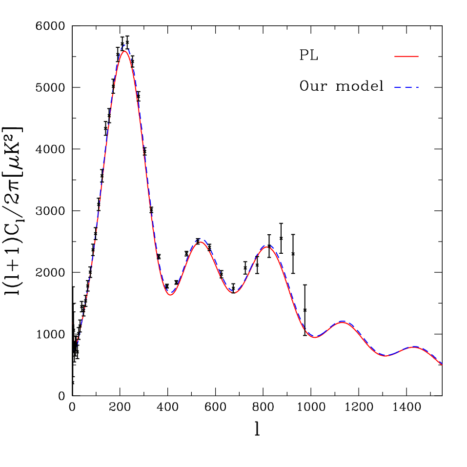
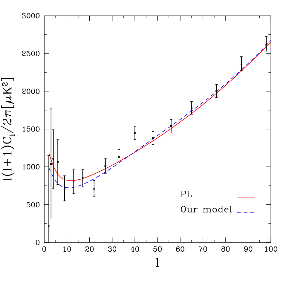
The package CosmoMC [14] was used to confront our model with the five-year observational data from WMAP. We find that our model gives a better fit with as compared to the best PL model with a constant . This improvement in the value of the likelihood has been obtained by introducing two more free parameters in our model as compared to the PL model, therefore it is reasonable. In fig. 4, the solid lines are marginalized probabilities of (the spectral index before the phase transition) and the dotted line gives the marginalized probabilities of (the spectral index after the phase transition). Observational data for multipoles with have been used. A contribution from primordial tensors, satisfying the one-inflaton consistency relation, , has been taken into account, too. The pivot point is set at .
From fig. 4 it is clear that a value of slightly larger than that without a step is favoured by the data. The marginalised probability for peaks at 0.947, while the marginalized probability for peaks at 0.97. Looking at the marginalized probability itself, we can see why a local running is suggested by our model: the peak of lies at a value significantly larger than . It is also interesting that the pair, favoured by CMB data, can be accommodated by the model (2.1) for very reasonable values of lying in the interval 40 - 60, as shown in fig. 1. In particular, to get just the peak values for and given above, one has to choose and that leads to .

The distributions for (red solid line) and also for (green dashed line) marginalized over all the other parameters are given in the left panel of fig. 5. It is quite clear from the plot that the data prefers be smaller than . Interestingly, the case corresponds to in our model. That is, the potential energy of the massive inflaton dominates the vacuum energy density at the moment of the phase transition. In the right panel of fig. 5 one can see the distribution of marginalized over all the other parameters. It is clear that the peak is at a value less than zero confirming the above result.
Note that in our previous theoretical paper [1], we were more concerned with the case since it leads to a larger value of , in particular, the spectrum even becomes blue-tilted for if . But observational data appear to have made their verdict for the opposite case when the potential is dominated by the term during the phase transition.
However, all formulae in [1] and in Sec. 2 are valid for any value of provided it is not very large. In more detail, the assumption of a fast phase transition is valid if during the transition, which requires (Eq. (4.9) of the paper [1]). For the typical values (see the table 1 in [1]), this leads to and , while corresponds to . It can be verified that if this condition is satisfied, then the contribution of particles created during this transition to the total energy density is small compared to the change in the equilibrium value of due to the step in its second derivative for the time period after the transition during which the correction (2.5-2.8) to the quasi-flat power spectrum is generated, irrespective of whether these created particles have decayed into other particles over this time period or not.
Another inequality bounding from above follows from the requirement that the change in the spectral index should be much more than next-order slow-roll corrections to and (not taken into account in our calculations), which are . This leads to . So, both upper limits on needed for the validity of Eq. (2.3) are effectively the same. Actually, they exclude the region only where the spectral feature itself becomes too small to be observable.


Fig. 6 gives the probability distribution for (location of the feature) which is larger for smaller values. It is clear that the feature, if exists at all, should preferentially lie on large scales: the marginalized upper limit for is 0.00355 Mpc-1 at 95% CL. Therefore, our model suggests that the main evidence for large running in the WMAP dataset comes from sufficiently low multipoles with .2 22footnotetext: Here we use the correspondence between and in the same form as the WMAP team: with Mpc.

Marginalized probabilities obtained for other cosmological parameters using the primordial spectrum given by our model are shown in fig. 7. It follows there are no significant changes in derived values of the cosmological parameters in comparison with the results, obtained by the WMAP team, assuming a power-law model of the primordial spectrum [4].

4 Conclusions and discussion
In this paper we confront the WMAP 5-year data with an exact solution [1] for the primordial power spectrum of perturbations generated when the inflaton effective potential has a sudden small change in its second derivative with respect to , i.e. in . The spectrum possesses a local universal feature having the form of a step in the primordial spectral index , modulated by comparatively weak oscillations (by universal is meant that the form of the spectral feature does not depend upon the structure of the discontinuity in ). It results in a large (but local) running of .
The simplest microscopic realization of such behaviour of is provided by a model having an auxiliary heavy scalar field which experiences a rapid second order phase transition (a mini-waterfall) during inflation in the observably accessible range of scales. Coupling this field to the inflaton leads to the desired type of local discontinuity in . The model is similar to that used in the hybrid inflationary scenario, but in contrast to the latter, its parameters are chosen in such a way that: (i) the transition occurs during inflation and not at its end, (ii) the change in the inflaton mass is small compared to the Hubble parameter at this moment. That is why we call it a ‘mini-waterfall’, in contrast to a ‘waterfall’ which provides an end to inflation in the hybrid scenario. Should such a mini-waterfall be detected through the corresponding feature in the primordial power spectrum of scalar perturbations, it would provide direct experimental evidence for the naturalness of a similar (though larger) waterfall in the hybrid scenario (the latter not being directly observable since it lies at a very small comoving scale).
We find that the best for this model shows an improvement by over the best fit obtained assuming a featureless power law for the primordial spectrum. (This improvement comes at the cost of introducing two additional parameters.) It is shown that such a feature in the primordial spectrum, if exists at all, should lie on large scales Mpc-1. Anyway, this feature is not excluded by the present observational data. Better data expected from future CMB experiments will help to settle the question about its existence.
An interesting problem not considered in this paper is the amount of non-Gaussianity in the statistics of primordial perturbations. Here, strictly speaking, one needs to distinguish two different, though related cases: the single-field inflationary model with an effective inflaton potential having the studied type of local non-analytic behaviour, and the two-field model (2.1). These models produce the same results for the power spectrum in the leading approximation, but may become non-equivalent at the level of deviations from Gaussian behaviour. Since the second field in the latter model is in the fast-rolling regime, one may expect larger amount of non-Gaussianity for it. We hope to return to this question elsewhere.
5 Acknowledgments
We acknowledge the use of high performance computing system at IUCAA. AAS acknowledges IUCAA hospitality as a visiting professor during the initial stage of this project. He was also partially supported by the grant RFBR 08-02-00923 and by the Scientific Programme “Elementary particles” of the Russian Academy of Sciences. MJ acknowledges the postdoctoral fellowship from KASI during the final stage of this project. A. S. acknowledges BIPAC and the support of the European Research and Training Network MRTPNCT-2006 10 035863-1 (UniverseNet).
References
- [1] M. Joy, V. Sahni and A. A. Starobinsky, Phys. Rev. D 77, 023514 (2008) (arXiv:0711.1585).
- [2] J. Lesgourgues, A. A. Starobinsky and W. Valkenburg, J. Cosm. Astropart. Phys. 0801, 010 (2008) (arXiv:0710.1630).
- [3]
D. N. Spergel, L. Verde, H. V. Peiris et al., Astroph. J. Suppl.
148, 175 (2003) (arXiv:astro-ph/0302209);
D. N. Spergel, R. Bean, O. Doré et al., Astroph. J. Suppl. 170, 377 (2007) (arXiv:astro-ph/0603449). - [4]
J. Dunkley, E. Komatsu, M.R. Nolta et al., Astrophys.J.Suppl. 180 (2009) (arXiv:0803.0586);
G. Hinshaw, J.L. Weinland, R.S. Hill et al., Astrophys.J.Suppl. 180 (2009) (arXiv:0803.0732). - [5] A. Benoit, P. Ade, A. Amblard et al., Astron. Astroph. 399, L25 (2003) (arXiv:astro-ph/0210306).
- [6]
R. Easther and H. Peiris, J. Cosm. Astropart. Phys. 0609, 010
(2006) (arXiv:astro-ph/0604214);
B. Feng, J.-Q. Xia and J. Yokoyama, arXiv:astro-ph/0608365. - [7]
L. A. Kofman and A. D. Linde, Nucl. Phys. B 282, 555 (1987);
L. A. Kofman and D. Y. Pogosyan, Phys. Lett. B 214, 508 (1988);
D. S. Salopek, J. R. Bond and J. M. Bardeen, Phys. Rev. D 40, 1753 (1989);
D. Polarski and A. A. Starobinsky, Nucl. Phys. B 385, 623 (1992);
H. V. Peiris, E. Komatsu, L. Verde et al., Astrophys. J. Suppl. 148, 213 (2003) (arXiv:astro-ph/0302225);
C. Contaldi, M. Peloso, L. Kofman and A. Linde, J. Cosm. Astropart. Phys. 0307, 002 (2003) (arXiv:astro-ph/0303636);
N. Kaloper and M. Kaplinghat, Phys. Rev. D 68, 123522 (2003) (arXiv:hep-th/0307016);
J. M. Cline and L. Hoi, J. Cosm. Astropart. Phys. 0606, 007 (2006) (arXiv:astro-ph/0603403). - [8]
A. A. Starobinsky, JETP Lett. 55, 489 (1992);
A. A. Starobinsky, in: ”Large Scale Structure: Tracks and Traces”, Proc. of the 12th Potsdam Cosmology Workshop (15-20 Sept. 1997), eds. V. Muller, S. Gottlober, J. P. Mucket, J. Wambsganss (Singapore: World Scientific), 1998, pp. 375-380 (arXiv:astro-ph/9808152). - [9]
J. A. Adams, G. G. Ross and S. Sarkar, Nucl. Phys. B 503, 405
(1997) (arXiv:hep-ph/9704286);
J. A. Adams, B. Cresswell and R. Easther, Phys. Rev. D 64, 123514 (2001) (arXiv:astro-ph/0102236);
P. Hunt and S. Sarkar, Phys. Rev. D 70, 103518 (2004) (arXiv:astro-ph/0408138);
S. Sarkar, Nucl. Phys. B Proc. Suppl. 148, 1 (2005) (arXiv:hep-ph/0503271);
P. Hunt and S. Sarkar, Phys. Rev. D 76, 123504 (2007) (arXiv:0706.4503). - [10] J.-O. Gong, J. Cosm. Astropart. Phys. 0507, 015 (2005) (arXiv:astro-ph/0504383).
- [11] M. Yamaguchi and J. Yokoyama, Phys. Rev. D 74, 043523 (2006) (arXiv:hep-ph/0512318).
- [12]
M. Tegmark and M. Zaldarriaga, Phys. Rev. D 66, 103508 (2002)
(arXiv:astro-ph/0207047) ;
M. Matsumiya, M. Sasaki and J. Yokoyama, Phys. Rev. D 65, 083007 (2002) (arXiv:astro-ph/0111549); ibid, J. Cosm. Astropart. Phys. 0302, 003 (2003) (arXiv:astro-ph/0210365) ;
S. L. Bridle, A.M. Lewis, J. Weller and G. Efsathiou, Mon. Not. Roy. Astron. Soc. 342 L72 (2003) (arXiv:astro-ph/0302306);
P. Mukherjee and Y. Wang, Astrophys. J. 599, 1 (2003) (arXiv:astro-ph/0303211) ;
S. Hannestad, J. Cosm. Astropart. Phys. 0404, 002 (2004) (arXiv:astro-ph/0311491) ;
A. Shafieloo and T. Souradeep, Phys Rev. D 70, 043523 (2004) (arXiv:astro-ph/0312174);
N. Kogo, M. Matsumiya, M. Sasaki and J. Yokoyama, Astrophys. J. 607, 32 (2004) (arXiv:astro-ph/0309662);
N. Kogo, M. Sasaki and J. Yokoyama, Prog. Theor. Phys. 114, 555 (2005) (arXiv:astro-ph/0504471);
P. Mukherjee and Y. Wang, J. Cosm. Astropart. Phys. 0512, 007 (2005) (arXiv:astro-ph/0502136);
D. Tocchini-Valentini, Y. Hoffman and J. Silk, Mon. Not. Roy. Astron. Soc. 367, 1095 (2006) (arXiv:astro-ph/0509478);
S. Leach, Mon. Not. Roy. Astron. Soc. 372, L646 (2006) (arXiv:astro-ph/0506390) ;
R. Sinha and T. Souradeep, Phys. Rev. D 74, 043518 (2006) (arXiv:astro-ph/0511808);
L. Covi et al., Phys.Rev. D 74, 083509 (2006) (arXiv:astro-ph/0606452);
A. Shafieloo, T. Souradeep, P. Manimaran et al., Phys. Rev. D 75, 123502 (2007) (arXiv:astro-ph/0611352);
J. Hamann, L. Covi, A. Melchiorri and A. Slosar, Phys. Rev. D 76, 023503 (2007) (arXiv:astro-ph/0701380);
A. Shafieloo and T. Souradeep, Phys. Rev. D 78, 023511 (2008) (arXiv:0709.1944).;
R. K. Jain et al., arXiv:0809.3915 - [13] A. D. Linde, Phys. Rev. D 49, 748 (1994) (arXiv:astro-ph/9307002).
- [14]
http://cosmologist.info/cosmomc/
A. Lewis and S. Bridle, Phys. Rev. D 66, 103511 (2002) (arXiv:astro-ph/0205436). - [15] E. Komatsu, J. Dunkley, M.R. Nolta et al., arXiv:0803.0547.