Disorder-driven splitting of the conductance peak at the Dirac point in graphene

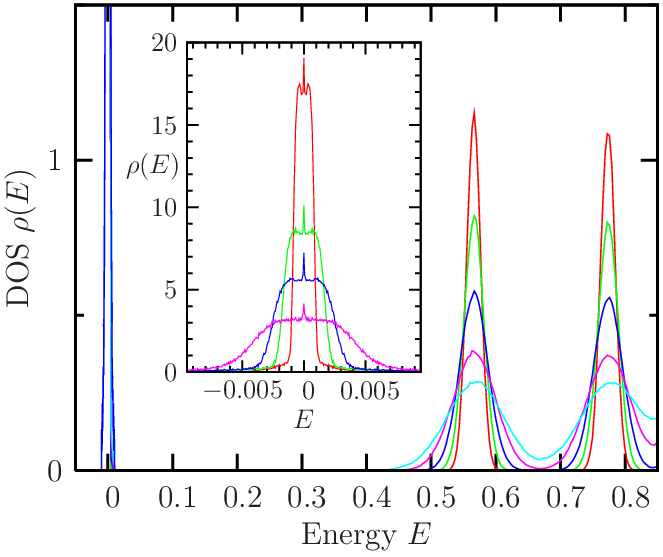
The density of states $\rho(E)$ was calculated by counting the eigenvalues obtained from diagonalization of $L^{2}=128\times 128$ samples with periodic boundary conditions in both directions, averaged over 500 disorder realizations. Without disorder, $\rho(E)$ was checked to be identical with the result of a true honeycomb lattice. Figure 2 shows $\rho(E)$ for $p/q=1/32$ flux quantum and several disorder strengths $f=0.001,0.002,0.003,\textnormal{and\ }0.005$. Due to the symmetry around $E=0$, the density of states is shown only for energies $E\gtrsim 0$. The Landau spectrum and the broadening of the bands are visible. However, compared with the $n=1$ and $n=2$ Landau bands, the central $n=0$ one remains very narrow and is hardly discernible. Therefore, in the inset of Fig. 2, the broadening of the narrow central band is shown in more detail where also the chiral peak at $E=0$ is distinguishable in the middle of the broadened Landau band. A real splitting of the $n=0$ Landau band becomes apparent only for very small disorder strength $f$. The total width at half height of the central band (neglecting the narrow chiral peak) is proportional to $\sqrt{p/q}f$. It should be noted that the degeneracy of the $n=0$ Landau level found in the Dirac model, even in the presence of a random magnetic field,[34] is already lifted in our clean lattice model due to Harper’s broadening.[35] In the case $B=0$, this lattice effect also causes deviations from the linear energy dispersion away from the Dirac point.

Since the number of eigenvalues is the same for each principle band shown in Fig. 2, the two split $n=0$ sub-bands must contain less eigenvalues than the higher Landau bands due to the additional chiral states close to the Dirac point $E=0$.

The energy dependence of the disorder averaged two-terminal conductance is shown in Fig. 3 for different random magnetic-field disorder strengths $f$. Again, only the positive energies are shown, because the conductance is an even function of the energy $E$. With increasing $f$, the conductance peaks corresponding to the $n=0$ Landau level, with peak value of about $1.12\,e^{2}/h$, move away from $E=0$, where the conductance peak of the scale independent chiral state remains fixed at $g(E=0)=1.27\,e^{2}/h$. The disorder induced splitting $\Delta E$ of the $n=0$ conductance peak is plotted in Fig. 4 versus $f$ for various magnetic fields with $p/q=1/24,1/32,1/64,\textnormal{ and }1/128$. For not too large $f$, the data points follow the straight solid lines which are given by the relation

Therefore, the conductance peak splitting shows a $\sqrt{B}$ behavior as observed in experiments and increases linearly with the strength $f$ of the random magnetic-flux disorder. Neither a splitting nor any shift of the conductance peak due to the disorder $f$ investigated could be observed for the $n=1$ Landau band and $L\leq 256$.

As known from experiment,[36] the minimum conductivity at the Dirac point depends verifiably on disorder. Therefore, in Fig. 5 we show the disorder dependence of the critical chiral conductance $\langle g(E=0,f)\rangle$ for different magnetic fields. The two values $4/\pi\,(e^{2}/h)$ and $8/\pi\,(e^{2}/h)$ are indicated by solid horizontal lines. The conductance turns out to be scale invariant for sufficiently strong random flux disorder. In the limit of $f\to 1.0$, $\langle g(E=0)\rangle$ converges to a common value that is a little larger than $8/\pi\,(e^{2}/h)$, which is independent of magnetic field. In contrast, a magnetic field dependence is seen for small $f$. In the range $0.001<f<0.4$, the conductance seems to approach a value somewhat smaller than $4/\pi\,(e^{2}/h)$ for all magnetic fields $p/q<1/32$ studied. For small disorder, e.g., $f=0.1$ and $B=0$, the conductance scales with the sample size. A convergence to a value $\approx 4/\pi\,(e^{2}/h)$ as in the finite $B$ case is compatible with our data.

In a finite clean system, $\langle g(E=0,f=0)\rangle$ is zero for $B=0$ but increases with the system size for finite $B$. The former behavior is due to the vanishing density of states at $E=0$ in the absence of a magnetic field. In the thermodynamic limit, the result for the conductance seems to depend on the order of limits $L\to\infty$ and $f\to 0$. A special case appears in the clean limit if $L_{z}$ is a multiple of three. $\langle g(E=0,f=0)\rangle$ turns out to be $2e^{2}/h$ due to the four eigenstates appearing at $E=0$ for $k_{z}=\pi/3$, where $k_{z}=N\pi/L_{z}$ and $N=1,2,\ldots$ . This agrees well with the experimentally observed minimal conductivity $\sigma_{\rm min}=4e^{2}/h$ if the electron spin is taken into account.

The energetic position of the split conductance peak within the $n=0$ Landau band as shown in Fig. 3 was estimated from the energy and size dependences of the conductance peak. For all values of disorder strength $f$, the conductance $g(E)$ exhibits a maximum around the critical energy $E_{c}(f)$. The maximal value of the conductance is $g_{c}\approx 1.12\,e^{2}/h$. If we take into account the factor of two due to the special aspect ratio, this value is in agreement with the critical conductance $g_{c}=0.6\,e^{2}/h$ found on the square lattice with spatial correlated diagonal disorder.[37] Likewise, it compares well with the results $g_{c}=2/\pi\,e^{2}/h$ obtained within a self-consistent Born approximation by Shon and Ando[38] for a graphene sheet in the presence of short- or long-range scattering potentials. Finally, our result for the split conductance peak agrees also with the analytical calculations of Ostrovsky and co-workers.[13, 15, 16]

A more detailed analysis of the size and energy dependences of the conductance shows that $g(E)$ exhibits a pronounced maximum around the disorder dependent critical energy $E_{c}(f)$. This renders the estimation of the corresponding critical exponent possible. The peak $g(E,f)$ becomes narrower when the size $L$ of the system increases. Following the scaling theory of localization, the conductance is assumed to be a function of only one parameter in the vicinity of the critical point, $\langle g\rangle=F[L/\xi(E)]$, with a diverging correlation length $\xi(E)\propto|E-E_{c}|^{-\nu}$. Then, we can extract the critical value of the conductance and the critical exponent assuming that

and

Figure 6 shows the size and energy dependence of the conductance peak for disorder $f=0.1$. We obtained a critical exponent $\nu\approx 2.5$ when only the data for $L\geq 384$ were used in the scaling analysis. We observed a similar behavior for smaller disorder strength $f=0.01$. In view of the uncertainties, we consider this to be consistent with the well-known results $\nu=2.3$ for ordinary quantum Hall systems supporting the view of the universality of the continuous quantum Hall phase transition.

The two-terminal conductance for the $n=1$ Landau band is shown in Fig. 7 versus energy. The peak value is about $1.87\,e^{2}/h$. The maximal available size of the system ($L=512$) is still insufficient for a more accurate estimation of the critical parameters. Therefore, we can neither give any limiting value nor address the Landau-level dependence of the critical conductance. The very slow $L$ dependence of the conductance in the critical region, indicating a larger localization length than for the $n=0$ case, makes the scaling analysis and estimation of critical exponent impossible.

From the energy and size dependences of the mean conductance in the vicinity of the chiral critical point we extract the critical conductance, $g_{c}=\lim_{L\to\infty}\langle g(E=0,L)\rangle$. Our data for the mean conductance $\langle g\rangle$ at the band center $E=0$ exhibit a convergence to the size independent limit $g_{c}$,

As shown in the inset of Fig. 8, $g_{c}$ $\simeq 1.267\,e^{2}/h$. This perfectly agrees with the theoretically predicted value $4/\pi\,e^{2}/h=1.273\,e^{2}/h$ for the spin-degenerate situation.[13, 15, 16] We mention again that in our case the factor of two originates not from the spin but from the special aspect ratio used.

To estimate the conductance fluctuations, we calculated the probability distribution $p(g)$ which proved to be Gaussian, confirming the presence of mesoscopic fluctuations also at the chiral critical point. The variance var $g=\langle g^{2}\rangle-\langle g\rangle^{2}$ varies slightly as a function of $B$ and $f$. For instance, we found var $g\approx 0.23\,(e^{2}/h)^{2}$ for the data shown in Fig. 8 but $0.21\,(e^{2}/h)^{2}$ for the $B=0$ case (Fig. 9).

To analyze the critical behavior of the conductance in the vicinity of the band center, we calculated $\langle g\rangle$ for square samples of size $L=64$, 128, 192, 256, and 384, within the narrow energy interval $10^{-9}\leq E\leq 10^{-4}$. Our data confirm that, after finite-size correction (7), the mean conductance is a function of one parameter only, $\langle g(E,L)\rangle=G(EL^{1/\nu})$. Following scaling theory, $\nu$ is the critical exponent that governs the divergence of the correlation length, $\xi(E)\propto|E|^{-\nu}$. A more detailed analysis shows that

with $c_{0}=0.05$, $c_{1}=-0.02944$, and $c_{2}=0.02134$. Scaling analysis provides us with the critical exponent $\nu=0.33\pm 0.1$. Although the best scaling is obtained for $\nu=0.33$ (as shown in Fig. 8), a reasonable scaling is also possible for values of the critical exponent in the range $0.25<\nu<0.45$. Again, only numerical data for much larger systems would reduce this inaccuracy.

We have carefully checked that our estimate of $\nu$ is insensitive to the range of the energy interval selected. Also, we tried to compensate for the observed divergence of the critical density of states near $E=0$, which, however, changed our estimates only marginally. We mention that our result does not satisfy the Harris criterion,[39] which states that $d\nu-2\geq 0$. There are similar results also for other models[40, 41, 42, 43, 44, 45] with chiral critical exponents $\nu<1$.

In the absence of a constant magnetic field, we observed that the value of the conductance at $E=0$ depends considerably on the size of the system, $g(L)=2.62-11.48/L$. Even worse, the scaling behavior is fulfilled only in a very narrow interval of conductance values. From Fig. 9 we see that the width of the scaling interval is comparable with the uncertainty in the conductance due to the finite-size effects. It is therefore no surprise that the estimation of the critical exponent is much more difficult. Taking into account these restrictions, we conclude that the estimated value of the critical exponent $\nu\approx 0.42$ is still in reasonable agreement with the previously obtained values $\nu=0.35$ and $\nu=0.42$ for a normal square lattice.[44, 45]

The critical eigenfunctions $\psi_{E}(r)$ of bricklayer samples with sizes up to $L^{2}=384\times 384$ were obtained numerically using a Lanczos algorithm. For eigenvalues close to $E=0$, the chiral eigenstates show the expected sub-lattice polarization, since for a clean system the wave functions are non-zero only on one of the sub-lattices.[25, 46] This sublattice polarization is still observable in the presence of both the fluctuating random flux and the constant perpendicular magnetic field. We also notice some weak quasi-one-dimensional structures making the appearance of $|\psi_{E=0}(r)|^{2}$ look slightly anisotropic.

A similar behavior is found for the $n=0$ critical quantum Hall states, as well. This is shown in Fig. 10 where the squared amplitude of a characteristic eigenstate with energy $E=0.016815$ is displayed for a $L=320$ sample with $p/q=1/32$ and RMF strength $f=0.1$. A closer inspection reveals an approximate sub-lattice polarization, also in this case. This effect appears to be stronger than in the diagonal disordered situation.[46]

The multifractal analysis was carried out as usual by utilizing the well-known box counting method where the scaling of a “box-probability” is calculated, $P(s,\lambda)=\sum_{i}^{N(l)}(\sum_{r\in\Omega_{i}(l)}|\psi_{E}(r)|^{2})^{s}\sim\lambda^{\tau(s)}$, from which the generalized fractal dimensions $D(s)=\tau(s)/(s-1)$ or, by a Legendre transform, the so-called $f[\alpha(s)]$ distribution can be derived.[47, 48] Here, $\Omega_{i}(l)$ is the $i$th box of size $l=\lambda L$ from which the $s$th moment of the modulus of the normalized eigenstate $\psi_{E}(r)$ is taken.

In Fig. 11 we show the $f[\alpha(s)]$ distribution of two $d=2$ chiral eigenstates at $E\approx 0$ in comparison with the parabolic approximation, $f[\alpha(s)]=d-[\alpha(s)-\alpha(0)]^{2}/\{4[\alpha(0)-d]\}$, which for finite systems is normally valid only for small $|s|$. We found a value $\alpha(0)=2.14\pm 0.02$ when averaged over several critical chiral states in the case $B=0$. This value turns out to be close to the one obtained previously for a square lattice with correlated random magnetic field.[49] For finite $B$, we found an averaged $\alpha(0)=2.27\pm 0.02$ which is the same as the $\alpha(0)$ value of the $n=0$ quantum Hall states. This result also agrees with $\alpha(0)$ values published for various quantum Hall models in the range $2.26<\alpha(0)\leq 2.29$.[50, 51, 52, 53] For the $n=1$ quantum Hall state the achievable system sizes were not sufficient for the calculation of a conclusive multifractal spectrum.

We finally mention that we also checked the $E=2.9725$ critical eigenstates within the Landau band closest to the tight-binding band edge in the presence of diagonal disorder. These outer states do not belong to the Dirac fermion sequence that can be found only in the energy range $-1.0\leq E\leq 1.0$. Again, we obtained the ordinary quantum Hall multifractality with $\alpha(0)\simeq 2.29$ and a critical conductance $g_{c}\simeq 1.0\,e^{2}/h$ (including the aspect ratio factor of 2).

References

- [1] K. S. Novoselov, A. Geim, S. V. Mozorov, D. Jiang, M. I. Katsnelson, I. V. Grigorieva, S. V. Dubonos, and A. A. Firsov, Nature 438, 197 (2005).
- [2] Y. Zhang, Y.-W. Tan, H. L. Stormer, and P. Kim, Nature 438, 201 (2005).
- [3] Y. Zhang, Z. Jiang, J. P. Small, M. S. Purewal, Y.-W. Tan, M. Fazlollahi, J. D. Chudow, J. A. Jaszczak, H. L. Stormer, and P. Kim, Phys. Rev. Lett. 96, 136806 (2006).
- [4] K. S. Novoselov, Z. Jiang, Y. Zhang, S. V. Morozov, H. L. Stormer, U. Zeitler, J. C. Maan, G. S. Boebinger, P. Kim, and A. K. Geim, Science 315, 1379 (2007).
- [5] A. J. M. Giesbers, U. Zeitler, M. I. Katsnelson, L. A. Ponomarenko, T. M. Mohiuddin, and J. C. Maan, Phys. Rev. Lett 99, 206803 (2007).
- [6] Z. Jiang, Y. Zhang, H. L. Stormer, and P. Kim, Phys. Rev. Lett. 99, 106802 (2007).
- [7] I. L. Aleiner and K. B. Efetov, Phys. Rev. Lett. 97, 236801 (2006).
- [8] A. Altland, Phys. Rev. Lett. 97, 236802 (2006).
- [9] S. V. Morozov, K. S. Novoselov, M. I. Katsnelson, F. Schedin, L. A. Ponomarenko, D. Jiang, and A. K. Geim, Phys. Rev. Lett. 97, 016801 (2006).
- [10] J. C. Meyer, A. K. Geim, M. I. Katsnelson, K. S. Novoselov, T. J. Booth, and S. Roth, Nature 446, 60 (2007).
- [11] A. F. Morpurgo and F. Guinea, Phys. Rev. Lett. 97, 196804 (2006).
- [12] F. Guinea, M. I. Katsnelson, and M. A. H. Vozmediano, Phys. Rev. B 77, 075422 (2008).
- [13] P. M. Ostrovsky, I. V. Gornyi, and A. D. Mirlin, Phys. Rev. B 74, 235443 (2006).
- [14] K. Nomura and A. H. MacDonald, Phys. Rev. Lett. 98, 076602 (2007).
- [15] P. M. Ostrovsky, I. V. Gornyi, and A. D. Mirlin, Eur. Phys. J. Spec. Top. 148, 63 (2007a).
- [16] P. M. Ostrovsky, I. V. Gornyi, and A. D. Mirlin, Phys. Rev. Lett. 98, 256801 (2007b).
- [17] D. V. Khveshchenko, EPL (Europhys. Lett.) 82, 57008 (2008).
- [18] D. A. Abanin, K. S. Novoselov, U. Zeitler, P. A.Lee, A. K. Geim, and L. S. Levitov, Phys. Rev. Lett. 98, 196806 (2007).
- [19] J.-N. Fuchs and P. Lederer, Phys. Rev. Lett. 98, 016803 (2007).
- [20] K. Nomura and A. H. MacDonald, Phys. Rev. Lett. 96, 256602 (2006).
- [21] D. A. Abanin, P. A. Lee, and L. S. Levitov, Phys. Rev. Lett. 96, 176803 (2006).
- [22] H. A. Fertig and L. Brey, Phys. Rev. Lett. 97, 116805 (2006).
- [23] M. O. Goerbig, R. Moessner, and B. Douçot, Phys. Rev. B 74, 161407(R) (2006).
- [24] J. Alicea and M. P. A. Fisher, Phys. Rev. B 74, 075422 (2006).
- [25] M. Koshino and T. Ando, Phys. Rev. B 75, 033412 (2007).
- [26] P. M. Ostrovsky, I. V. Gornyi, and A. D. Mirlin, Phys. Rev. B 77, 195430 (2008).
- [27] Y. Hasegawa, Y. Hatsugai, M. Kohmoto, and G. Montambaux, Phys. Rev. B 41, 9174 (1990).
- [28] K. Wakabayashi, M. Fujita, H. Ajiki, and M. Sigrist, Phys. Rev. B 59, 8271 (1999).
- [29] J. Miller and J. Wang, Phys. Rev. Lett. 76, 1461 (1996).
- [30] A. Furusaki, Phys. Rev. Lett. 82, 604 (1999).
- [31] C. Mudry, P. W. Brouwer, and A. Furusaki, Phys. Rev. B 59, 13221 (1999).
- [32] P. W. Brouwer, C. Mudry, B. D. Simons, and A. Altland, Phys. Rev. Lett. 81, 862 (1998).
- [33] J. B. Pendry, A. MacKinnon, and P. J. Roberts, Proc. R. Soc. London, Sect. A 437, 67 (1992).
- [34] Y. Aharonov and A. Casher, Phys. Rev. A 19, 2461 (1979).
- [35] P. G. Harper, Proc. Phys. Soc. London, Sect. A 68, 874 (1955).
- [36] Y.-W. Tan, Y. Zhang, K. Bolotin, Y. Zhao, S. Adam, E. H. Hwang, S. Das Sarma, H. L. Stormer, and P. Kim, Phys. Rev. Lett. 99, 246803 (2007).
- [37] L. Schweitzer and P. Markoš, Phys. Rev. Lett. 95, 256805 (2005).
- [38] N. H. Shon and T. Ando, J. Phys. Soc. Jpn. 67, 2421 (1998).
- [39] A. B. Harris, J. Phys. C: Solid State Phys. 7, 1671 (1974).
- [40] Y. Morita and Y. Hatsugai, Phys. Rev. B 58, 6680 (1998).
- [41] V. Z. Cerovski, Phys. Rev. B 62, 12775 (2000).
- [42] A. Eilmes, R. A. Römer, and M. Schreiber, Physica B 296, 46 (2001).
- [43] V. Z. Cerovski, Phys. Rev. B 64, 161101(R) (2001).
- [44] P. Markoš and L. Schweitzer, Phys. Rev. B 76, 115318 (2007).
- [45] L. Schweitzer and P. Markoš, Physica E 40, 1335 (2008).
- [46] A. L. C. Pereira and P. A. Schulz, Phys. Rev. B 77, 075416 (2008).
- [47] T. C. Halsey, M. H. Jensen, L. P. Kadanoff, I. Procaccia, and B. I. Shraiman, Phys. Rev. A 33, 1141 (1986).
- [48] A. Chhabra and R. V. Jensen, Phys. Rev. Lett. 62, 1327 (1989).
- [49] H. Potempa and L. Schweitzer, Ann. Phys. (Leipzig) 8, SI-209 (1999).
- [50] B. Huckestein, B. Kramer, and L. Schweitzer, Surf. Sci. 263, 125 (1992).
- [51] B. Huckestein and L. Schweitzer, Phys. Rev. Lett. 72, 713 (1994).
- [52] R. Klesse and M. Metzler, Europhys. Lett. 32, 229 (1995).
- [53] F. Evers, A. Mildenberger, and A. D. Mirlin, Phys. Rev. B 64, 241303(R) (2001).
- [54] K. Minakuchi and S. Hikami, Phys. Rev B 53, 10898 (1996).