Closed 1-forms in topology and dynamics
Abstract.
This article surveys recent progress of results in topology and dynamics based on techniques of closed one-forms. Our approach allows us to draw conclusions about properties of flows by studying homotopical and cohomological features of manifolds. More specifically we describe a Lusternik - Schnirelmann type theory for closed one-forms, the focusing effect for flows and the theory of Lyapunov one-forms. We also discuss recent results about cohomological treatment of the invariants and and their explicit computation in certain examples.
To S.P. Novikov on the occasion of his 70-th birthday
In 1981 S.P. Novikov [37, 40] initiated a generalization of Morse theory which gives topological estimates on the numbers of zeros of closed 1-forms, see also [42, 43]. Novikov was motivated by a variety of important problems of mathematical physics, leading, in one way or another, to the problem of finding relations between the topology of the underlying manifold and the number of zeros which closed 1-forms in a specific one-dimensional real cohomology class possess. Recall that a closed 1-form can be viewed as a multi-valued function or functional whose branching behavior is fully characterized by the cohomology class.
In [40] Novikov studies various problems of physics where the motion can be reduced to the principle of an extremal action , which is a multi-valued functional on the space of curves, with the variation being a well-defined closed 1-form, cf. [39, 38, 41]. Among problems of this kind are the Kirchhoff equations for the motion of a rigid body in ideal fluid, the Leggett equation for the magnetic momentum, and others.
His fundamental idea in [40] was based on a plan to construct a chain complex, now called the Novikov complex, which uses dynamics of the gradient flow in the abelian covering associated with the cohomology class. The dynamics of gradient flows appears traditionally in Morse theory providing a bridge between the critical set of a function and the global ambient topology.
At present the Novikov theory of closed one-forms is a rapidly developing area of topology which interacts with various mathematical theories. J.-Cl. Sikorav [56, 57] was the first who applied Novikov theory in symplectic topology. Hofer and Salamon [29] pioneered exploiting the ideas of Novikov theory in Floer theory. More recent applications of Novikov theory in symplectic topology and Hamiltonian dynamics can be found, for example, in the work of Oh [44], Usher [63] and references mentioned there. Combinatorial group theory is another area where Novikov theory plays an important role; this connection was also discovered by J.-Cl. Sikorav who realized that the Bieri - Neumann - Strebel invariant can be expressed in terms of (a generalized noncommutative) Novikov homology.
Many problems of Novikov theory are still being actively developed in current research. The list of such topics includes (a) constructions of chain complexes (more general than the Novikov complex) which are able to capture the link between topology of the manifold and topology of the set of zeros, (b) various types of inequalities for closed 1-forms (with Morse or Bott type nondegeneracy assumptions), (c) equivariant inequalities and (d) problems about sharpness of these inequalities.
Topology of closed 1-forms is a broader research area which together with the Novikov theory studies a new Lusternik - Schnirelmann type theory for closed 1-forms initiated in 2002 in [16]. The latter theory also aims at finding relations between topology of the zero set of a closed one-form and homotopy information, based mainly on the cohomology class of the form. The words “Lusternik - Schnirelmann type” intend to emphasize that no assumptions on the character of zeros are made, unlike the ones which appear in the Novikov theory requiring that all zeros are nondegenerate in the sense of Morse.
Although Lusternik - Schnirelmann theory for closed one-forms shares many common features with the Lusternik - Schnirelmann theory of functions and with the Novikov theory of closed one-forms, it is also very different from both these classical theories. The most striking new phenomenon is based on the fact that in any nonzero cohomology class there always exists a closed 1-form having at most one zero (see Theorem 4 below). Hence, the new theory is not merely about the number of zeros but, as we show in this article, about qualitative dynamical properties of smooth flows on manifolds.
Given a smooth flow one wants to “tame” it by a closed 1-form lying in a prescribed cohomology class. More precisely, one wants to find a closed 1-form such that the flow is locally decreasing. This idea leads to the notion of a Lyapunov closed one-form generalizing the classical notion of a Lyapunov function. The key question about the existence of Lyapunov closed 1-forms for flows has been resolved in a series of papers of Farber, Kappeler, Latschev and Zehnder [17, 20, 21, 33, 34]. Note that the classical theorem of C. Conley [5, 6] gives the answer in the special case of the zero cohomology class, i.e. when one deals with Lyapunov functions. When the cohomology class is nontrivial the notion of asymptotic cycle of a flow introduced by Schwartzman [53, 54] plays a crucial role.
A brief account of Lusternik - Schnirelmann theory for closed one-forms can be found in chapter 10 of the book [19] published in 2004. The main idea of this paper is to survey the new results obtained after 2004. To put the material in context we start this survey with a section describing the basic results of the Novikov theory.
In a forthcoming paper [27] we introduce and study the notion of sigma invariants for a finite CW-complex analogously to the sigma invariants of groups of Bieri et al [2, 3]. These invariants carry information about the finiteness properties of infinite abelian covers of . Both the present survey and [27] have a common main theme: they are based on movability properties of subsets of with respect to a closed 1-form which are very close in spirit to the idea of Novikov homology.
Table of contents
1. Fundamentals of the Novikov theory
2. The colliding theorem
3. Closed 1-forms on general topological spaces
4. Lyapunov 1-forms for flows
5. Notions of category with respect to a cohomology class
6. Focussing effect
7. Existence of flow-convex neighbourhoods
8. Proof of Theorem 12
9. Topology of the chain recurrent set
10. Proof of Theorem 14
11. Cohomological estimates for
12. Upper bounds for and relations with the Bieri - Neumann - Strebel invariants
13. Homological category weights, estimates for and calculation of , for products of surfaces
1. Fundamentals of the Novikov theory
S.P. Novikov [37], [40] suggested a generalization of the classical Morse theory which gives lower bounds on the number of zeros of Morse closed 1-forms. In this section we will give a brief account of the Novikov theory. We touch here only the following selected topics: Novikov inequalities, Novikov numbers, and Novikov Principle leading to the notion of the Novikov complex. We refer the reader to the original papers [37, 40] and to the monograph [19] for proofs and more details. Historical information about the development of the subject after [37, 40] as well as bibliographic references can also be found in [19].
1.1. Novikov inequalities
Let be a smooth manifold. A smooth closed 1-form on is defined as a smooth section of the cotangent bundle satisfying . By the Poincaré lemma for any simply connected open set one has where is a smooth function, defined uniquely up to addition of a locally constant function. The zeros of are points such that . If lies in a simply connected domain then if and only if is a critical point of .
Definition 1.
A zero of a smooth closed 1-form is said to be non-degenerate if it is a non-degenerate critical point of the function .
Clearly, this property is independent of the choice of the simply connected domain and the function .
Definition 2.
The Morse index of a non-degenerate zero of is defined as the Morse index of viewed as a critical point of .
We denote the Morse index by . It takes values where .
The main problem of the Novikov theory is as follows. Let be a smooth closed one-form on a closed smooth manifold . Let us additionally assume that is Morse, i.e. all its zeros are nondegenerate in the sense explained above. We denote by the number of zeros of having Morse index , where . One wants to estimate the numbers in terms of information about the topology of and of the cohomology class
| (1) |
represented by .
In the case of classical Morse theory one has (i.e. where is a smooth function) and the answer is given by the Morse inequalities
| (2) |
where denotes the -th Betti number of and denotes the minimal number of generators of the torsion subgroup of .
S.P. Novikov [37, 40] introduced generalizations of the numbers and which depend on the cohomology class of (see (1)) and are denoted and correspondingly. We call the Novikov - Betti number; the number is the Novikov torsion number. Their definitions will be given below. The Novikov inequality (in its simplest form) states:
Theorem 1.
Let be a smooth closed 1-form on a smooth closed manifold . Assume that all zeros of are nondegenerate. Then
| (3) |
where denotes the cohomology class represented by .
Note that for the number coincides with and the number coincides with , i.e. the Novikov inequalities (3) contain the Morse inequalities (2) as a special case.
Our goal in this section is to explain the main ideas of the proof of Theorem 1 without intending to present full details. A complete proof can be found in [19], pages 46 - 48.
Next we introduce the Novikov ring where is a commutative ring. Elements of are formal “power series” of the form
where is a formal variable, the coefficients are elements of , , and the exponents are arbitrary real numbers satisfying the following condition: for any the set
| (4) |
is finite. Equivalently, an element can be represented in the form
where , , and tends to . In other words, element of the Novikov ring are “Laurent like” power series with integral coefficients and with arbitrary real exponents tending to .
Addition in is given by adding the coefficients of powers of with equal exponents. Multiplication in is given by the formula
where
Note that the last sum contains only finitely many nonzero terms and moreover, the set of all the exponents for which is nonzero also satisfies the property that the sets (4) are finite.
For simplicity, we will abbreviate the notation to .
Lemma 1.
The ring is a principal ideal domain. Moreover, for any field the ring is a field.
The second statement is in fact trivial; the proof of the first statement can be found in [19], page 8. The credit for Lemma 1 should be mainly given to S.P. Novikov who discovered and stated it without proof. Full proofs appear in [29], [45] and [19]. Similar statements concerning related rings of rational functions were discovered in [12], [56].
Now we can explain how one associates to a cohomology class the Novikov numbers and . Here we assume that is a smooth closed manifold although the construction is applicable to finite polyhedra. Consider the group ring where denotes the fundamental group . The class determines a ring homomorphism
| (5) |
defined on a group element by the formula
Here is the evaluation of the cohomology class on the homotopy class . Recall that denote the formal indeterminant of the Novikov ring. Clearly,
i.e. is multiplicative on group elements. It follows that extends by linearity on the whole group ring as a ring homomorphism. By the well-known construction homomorphism (5) defines a local system of left -modules over which we denote by . The homology of this local system is a finitely generated module over the Novikov ring . As we know, is a principal ideal domain, and therefore is a direct sum of a free and a torsion -module.
Definition 3.
The Novikov-Betti number is defined as the rank of the free part of . The Novikov torsion number is defined as the minimal number of generators of the torsion submodule of .
Recall the definition of homology of local system . Consider the universal cover and the singular chain complex . The latter is a chain complex of free left modules over the group ring . One views as a right -module where
Then is the homology of the chain complex
| (6) |
1.2. Novikov and Universal complexes
The main idea of S.P. Novikov in [37, 40] which finally led him to Theorem 1 was the statement that for any Morse closed 1-form on a smooth closed manifold there exists a chain complex (which is now known as the Novikov complex) having the following two properties:
- (1)
is a free chain complex of -modules and each module has a canonical free basis which is in one-to-one correspondence with zeros of having Morse index , where .
- (2)
is chain homotopy equivalent to the complex . In particular, the homology is isomorphic to .
This statement, which we call the the Novikov Principle, trivially implies Theorem 1. It should be compared with the classical Morse Principle which claims that for any Morse function on a closed smooth manifold there exists a chain complex having the following two properties:
- (1)
is a free chain complex of -modules and each module has a canonical free basis which is in one-to-one correspondence with critical points of having Morse index , where .
- (2)
is chain homotopy equivalent to the chain complex , where is the universal cover of and .
There are several explicit constructions of Morse theory which lead to the complex . One of them is based on the fact that admits a cell-decomposition with cells in one-to-one correspondence with critical points of . Another well-known construction of is based on the Witten deformation of the de Rham complex.
One is naturally led to ask if there exist other ring homomorphisms
| (7) |
distinct from (5), for which the analogue of the Novikov Principle holds. To be more specific, we say that the Novikov Principle is valid for a group , a group homomorphism11 1 One has for and a ring homomorphism if for any smooth closed manifold with and for any Morse closed 1-form on representing the cohomology class there exists a chain complex
of free finitely generated -modules having the following two properties:
- (1)
each module has a canonical free basis which is in one-to-one correspondence with the zeros of having Morse index ;
- (2)
The complex is chain homotopy equivalent to , where is viewed as a left -module via .
A positive answer to this question was given in [13] in the case of rational cohomology classes and in [15] in the general case. Besides (5) the Novikov principle holds for many other ring homomorphisms (7). Moreover, there exists “the largest” such homomorphism which we describe below. The chain complex in this case is called the Universal complex. This complex lives over a localization of the group ring .
An element will be called -negative if (finite sum), where and for all . An -matrix over the group ring will be called -negative if all its entries are -negative. Consider the class of square matrices of the form , where is an arbitrary -negative square matrix with entries in .
Note that in the case (when one studies Morse functions) the set of -negative matrices is empty and so the Cohn localization (8) is just the identity map.
We will use the notion of noncommutative localization developed by P.M. Cohn [4]. The universal Cohn localization of the group ring with respect to the class is a ring together with a ring homomorphism
| (8) |
satisfying the following two properties: first, any matrix , where is -negative, is invertible over , and, secondly, it is a universal homomorphism having this property, i.e., for any ring homomorphism , inverting all matrices of the form , where is -negative, there exists a unique ring homomorphism such that the following diagram commutes
Theorem 2.
Let be any group and be a cohomology class. Then the Novikov Principle is valid for the Cohn localization (8).
Farber and Ranicki in [13] proved this theorem in the case of integral cohomology classes; the general case was treated by Farber [14]. The construction of the Universal complex employs the technique of collapse for chain complexes which is analogous to the well-known operation of combinatorial collapse. This technique was initiated in [13].
One should mention another important closely related ring called the Novikov-Sikorav completion ; it was first introduced by J.-Cl. Sikorav [56] who was inspired by the construction of the Novikov ring . One can view as the noncommutative analogue of the Novikov ring. Elements of are represented by formal sums, possibly infinite,
where and , satisfying the following condition: for any real number the set is finite. Compare this with the construction of the Novikov ring above. Addition and multiplication are given by the usual formulae; for example, the product of and is given by
| (9) |
The ring homomorphism is the inclusion. If is a -negative square matrix over the ring , then the power series
converges in and hence the matrix is invertible in . From the universal property of the Cohn localization it follows that there exists a canonical ring homomorphism
| (10) |
extending the inclusion . This implies that the homomorphism (8) is injective.
1.3. Novikov numbers and the fundamental group
It is obvious that one-dimensional Novikov numbers and depend only on the fundamental group and on the homomorphism of periods . Interestingly there is also a strong inverse dependence, i.e. one may sometimes recover information about the fundamental group while studying and . The following result shows that nontriviality of the first Novikov - Betti number happens only if the fundamental group is “large”:
Theorem 3 (Farber-Schütz [22]).
Let be a connected finite complex and let be a nonzero cohomology class. If the first Novikov-Betti number is positive then contains a nonabelian free subgroup.
Theorem 3 has the following Corollaries:
Corollary 2.
Let be a connected finite polyhedron having an amenable fundamental group. Then the first Novikov-Betti number vanishes for any .
Corollary 3.
Assume that is a connected finite two-dimensional polyhedron. If the Euler characteristic of is negative then contains a nonabelian free subgroup.
2. The colliding theorem
As follows from the discussion of the previous section, the Novikov theory gives bounds from below on the number of distinct zeros which have closed Morse type 1-forms lying in a prescribed cohomology class . The total number of zeros is then at least the sum of the Novikov numbers .
If is a closed 1-form representing the zero cohomology class then where is a smooth function; in this case must have at least geometrically distinct zeros (which are exactly the critical points of the function ), according to the classical Lusternik-Schnirelmann theory [8]; this result requires no assumptions on the nature of the zeros.
Encouraged by the success of the Novikov theory one may ask if it is possible to construct an analogue of the Lusternik - Schnirelmann theory for closed 1-forms. It is quite surprising that in general, with the exception of two situations mentioned above, there are no obstructions for constructing closed 1-forms possessing a single zero. Hence, for , the only homotopy invariant (depending on the topology of and on the cohomology class ) such that any closed 1-form on with has at least zeros is or .
Theorem 4 (Farber [16], Farber - Schütz [23]).
Let be a closed connected -dimensional smooth manifold, and let be a nonzero real cohomology class. Then there exists a smooth closed 1-form in the class having at most one zero.
This result suggests that “the Lusternik-Schnirelmann theory for closed 1-forms” (if it exists) must have a new character, quite distinct from both the classical Lusternik-Schnirelmann theory of functions and the Novikov theory of closed 1-forms.
Theorem 4 was proven in [16] under an additional assumption that the class is integral, ; see also [19], Theorem 10.1. In full generality it was proven in [23].
Let us mention briefly a similar question. We know that if then there exists a nowhere zero 1-form on . Given , one may ask if it is possible to find a nowhere zero 1-form on which is closed, i.e. ? The answer is negative in general. For example, vanishing of the Novikov numbers is a necessary condition for the class to be representable by a closed 1-form without zeros. The full list of necessary and sufficient conditions (in the case ) is given by the theorem of Latour [35].
Theorem 4 was proven in [16] and [19] in the case when the cohomology class is of rank 1. In this section we follow our recent paper [23] and give the proof of Theorem 4 in the case when .
2.1. Singular foliations of closed one-forms
Let be a smooth manifold. A smooth closed 1-form with Morse zeros determines a singular foliation on . It is a decomposition of into leaves: two points belong to the same leaf if there exists a path with , and for all . Locally, in a simply connected domain , we have , where ; each connected component of the level set lies in a single leaf. If is small enough and does not contain the zeros of , one may find coordinates in such that ; hence the leaves in are the sets . Near such points the singular foliation is a usual foliation. On the contrary, if is a small neighborhood of a zero of having Morse index , then there are coordinates in such that and the leaves of in are the level sets The leaf with contains the zero . It has a singularity at : a neighborhood of in is homeomorphic to a cone over the product . There are finitely many singular leaves, i.e. the leaves containing the zeros of .
We are particularly interested in the singular leaves containing the zeros of having Morse indices 1 and . Removing such a zero locally disconnects the leaf . However globally the complement may or may not be connected.
The singular foliation is co-oriented: the normal bundle to any leaf at any nonsingular point has a specified orientation.
We shall use the notion of a weakly complete closed 1-form introduced by G. Levitt [36]. A closed 1-form is called weakly complete if it has Morse type zeros and for any smooth path with the endpoints and lie in the same leaf of the foliation on . Here denotes where are the zeros of .
A weakly complete closed 1-form with has no zeros with Morse indices and . According to Levitt [36], any nonzero real cohomology class can be represented by a weakly complete closed 1-form.
The plan of our proof of Theorem 4 is as follows. We start with a weakly complete closed 1-form lying in the prescribed cohomology class , . We show that assuming all leaves of the singular foliation are dense (see §2.2). We perturb such that the resulting closed 1-form has a single singular leaf (see §2.3). After that we apply the technique of Takens [62] allowing us to collide the zeros in a single (highly degenerate) zero. We first prove Theorem 4 assuming that ; the special case is treated separately later.
2.2. Density of the leaves
In this section we show that if is weakly complete and then the leaves of are dense; moreover, given a point and a leaf of the singular foliation , there exist two sequences of points and such that , and
| (11) |
The integrals in (11) are calculated along an arbitrary path lying in a small neighborhood of . This can also be expressed by saying that the leaf approaches from both the positive and the negative sides. This statement was also observed by G. Levitt [36], p. 645; we give below a different proof. In general the assumptions that has no centers and do not imply that the leaves of the foliation are dense, see the examples in Chapter 11, §9.3 of [19].
Let be a weakly complete closed 1-form in class . Consider the covering corresponding to the kernel of the homomorphism of periods , where . Let be the group of periods. The rank of equals ; since we assume that , the group is dense in . The group of periods acts on the covering space as the group of covering transformations. We have where is a smooth function. The leaves of the singular foliation are the images under the projection of the level sets ; this property follows from the weak completeness of , see [36], Proposition II.1. For any and one has
| (12) |
Let be a leaf and let be an arbitrary point. Our goal is to show that lies in the closure of . Let be a path-connected neighborhood of which is assumed to be “small” in the following sense: . We want to show that contains a point satisfying where the integral is calculated along a curve in .
Consider a lift , . Let be a neighborhood of which is mapped by homeomorphically onto . We claim that the set of values contains an interval where and .
![[Uncaptioned image]](0807.3240v2/approx1.png)
This claim is obvious if is not a critical point of since in this case one may choose the coordinates around such that . In the case when is a critical point of , one may choose the coordinates near the point such that is given by and our claim follows since we know that the Morse index is distinct from and .
Because of the density of the group of translations one may find such that the real number lies in the interval . Then we obtain
| (13) |
We see that the sets and have a common point . The point has the required property .
2.3. Modification
Our next goal is to replace by a Morse closed 1-form which has the property that all its zeros lie on the same singular leaf of the singular foliation . In this section we assume that .
Let be a weakly complete Morse closed 1-form in class where . Let be the zeros of . For each choose a small neighborhood and local coordinates in such that for and
| (14) |
Here denotes the Morse index of . We assume that the ball is contained in and that for . Denote by the open ball .
Let be a smooth function with the following properties: (a) on ; (b) on ; (c) .
Such a function exists assuming that is small enough. (a), (b), (c) imply that
| (15) |
We replace the closed 1-form by
| (16) |
where is a smooth function with support in . In the coordinates of (see above) the function is given by The parameters appearing in (16) are specified later.
One has on and near the zeros of . Let us show that has no additional zeros. We have (where is defined in (14)) and
| (17) |
If this partial derivative vanishes and then which may happen only for according to (15).
We now show how to choose the parameters so that the closed 1-form given by (16) has a unique singular leaf. Let be a fixed nonsingular leaf of . Since is dense in (see §2.2) for any the intersection contains infinitely many connected components approaching from below and from above and the function is constant on each of them.
![[Uncaptioned image]](0807.3240v2/leaves.png)
We say that a subset is a level set if for some . Note that . The level set contains the zero ; it is homeomorphic to the cone over the product . Each level set with is diffeomorphic to and each level set with is diffeomorphic to . Recall that denotes the Morse index of .
Let denote the set of values of on different level sets belonging to the leaf . The zero does not lie in since we assume that the leaf is nonsingular. However, according to the result proven in §2.2, the zero is a limit point of and, moreover, the closure of either of the sets and contains .
For the modification (given by (16)) one has where . The level sets for are defined as . Clearly is given by the equation
Hence for this is the same as ; for the level set coincides with . In the ring the level set is homeomorphic to a cylinder.
The following figure illustrates the distinction between the level sets and in the case .
![[Uncaptioned image]](0807.3240v2/leaves3.png)
Examine the changes which the leaf undergoes when we replace by . Here we view with the leaf topology; it is the topology induced on from the covering using an arbitrary lift . First, let us assume that: (1) the Morse index satisfies ; (2) the coefficient is positive; (3) the number lies in the set . Then the complement
is connected and it lies in a single leaf of the singular foliation . We see that the new leaf is obtained from by infinitely many surgeries. Namely, each level set , where satisfies , is removed and replaced by a copy of ; besides, the set where , is removed and gets replaced by a cone over the product . Hence the new leaf contains the zero .
Let us now show how one may modify the above construction in the case . Since we have in this case ; hence removing the sphere from the leaf does not disconnect . We shall assume that the coefficient is negative and that the number lies in . The complement
is connected and it lies in a single leaf of the singular foliation . Clearly, is obtained from by removing the level sets where satisfies (each such is diffeomorphic to ) and by replacing them by copies of . In addition, the set where , is removed and is replaces by a cone over the product .
We see that is a leaf of the singular foliation containing all the zeros .
2.4. Proof of Theorem 4
Below we assume that . The case is covered by Theorem 2.1 from [16].
The results of the preceding sections allow us to complete the proof of Theorem 4 in the case . Indeed, we showed in §2.3 how to construct a Morse closed 1-form lying in the prescribed cohomology class such that all zeros of are Morse and belong to the same singular leaf of the singular foliation . Now we may apply the colliding technique of F. Takens [62], pages 203–206. Namely, we may find a piecewise smooth tree containing all the zeros of . Let be a small neighborhood of which is diffeomorphic to . We may find a continuous map with the following properties:
is a single point ;
is a diffeomorphism onto ;
is the identity map on the complement of a small neighborhood of where the closure is contained in .
Consider a smooth function such that ; it exists and is unique up to a constant. The function is well-defined (since is constant). is continuous by the universal property of the quotient topology. Moreover, is smooth on . Applying Theorem 2.7 from [62], we see that we can replace by a smooth function having a single critical point at and such that on .
Let be a closed 1-form on given by
| (18) |
Clearly is a smooth closed 1-form on having no zeros in . Moreover, lies in the cohomology class (since any loop in is homologous to a loop in ).
Now we prove Theorem 4 the case . We shall replace the construction of §2.3 (which requires ) by a direct construction. The final argument using the Takens’ technique [62] remains the same.
Let be a closed surface and let be a nonzero cohomology class. We can split into a connected sum
where each is a torus or a Klein bottle and such that the cohomology class is nonzero. Let be a closed 1-form on lying in the class and having no zeros; obviously such a form exists. §9.3.2 of [19] describes the construction of connected sum of closed 1-forms on surfaces. Each connecting tube contributes two zeros. In fact there are three different ways of forming the connected sum, they are denoted by A, B, C on Figure 9.8 in [19]. In the type C connected sum the zeros lie on the same singular leaf. Hence by using the type C connected sum operation we get a closed 1-form on having zeros which all lie on the same singular leaf of the singular foliation . The colliding argument based on the technique of Takens [62] applies as in the case and produces a closed 1-form with at most one zero lying in class .
3. Closed one-forms on general topological spaces
Since closed one-forms are central for our constructions, it will be convenient to operate with the notion of a closed one-form defined on general topological spaces. This notion will allow us to deal with spaces more general than smooth manifolds. The calculus of closed one-forms on topological spaces is very similar to that of smooth closed one-forms on manifolds: one may integrate any closed one-form along a path; the integral depends only on the homotopy class of the path; any closed one-form represents a one-dimensional cohomology class and any continuous function determines an exact closed one-form , the differential of .
In this section we recall the basic definitions referring to the book [19] for proofs and more details.
3.1. Basic definitions
Definition 4.
A continuous closed 1-form on a topological space is defined as a collection of continuous real-valued functions , where is an open cover of , such that for any pair the difference
is a locally constant function. Another such collection (where is another open cover of ) defines an equivalent closed 1-form if the union collection
is a closed 1-form (in the sense of the above definition), i.e., if for any and , the function is locally constant on .
Let be a continuous map and let be a continuous closed 1-form on . Then the induced closed 1-form is defined as follows. Let , where is an open cover of . The family is an open cover of and the functions define a continuous closed 1-form with respect to the cover .
As an example consider an open cover consisting of the whole space . Then any continuous function defines a closed 1-form on , which is denoted by . For two continuous functions , holds if and only if the difference is locally constant.
3.2. Integration
One may integrate continuous closed 1-forms along continuous paths. Let be a continuous closed 1-form on given by a collection of continuous real-valued functions with respect to an open cover of . Let be a continuous path. The line integral is defined as follows. Find a subdivision of the interval such that for any the image is contained in a single open set . Then we define
| (19) |
The standard argument shows that the integral (19) does not depend on the choice of the subdivision and the open cover .
For any pair of continuous paths with common beginning and common end points , it holds that
provided that and are homotopic relative to the boundary.
3.3. Cohomology class of a closed one-form
Any continuous closed 1-form defines the homomorphism of periods
| (20) |
given by integration along closed loops with . The image of this homomorphism is a subgroup of whose rank is called the rank of and is denoted .
Recall that a topological space is homologically locally -connected if for every point and any neighborhood of there exists a neighborhood of in such that the induced homomorphism of the reduced integral singular homology is trivial for all . is locally path connected iff it is homologically locally 0-connected.
Lemma 4.
Let be a locally path-connected topological space. A continuous closed 1-form on equals for a continuous function if and only if for any choice of the base point the homomorphism of periods (20) determined by is trivial.
Proof.
If , then holds for any path in , where . Hence if is a closed loop.
Conversely, assume that the homomorphism of periods (20) is trivial. Our assumption about implies that connected components of are open and path connected. In each connected component of choose a base point . One defines a continuous function by
here and belong the same connected component of and the integration is taken along an arbitrary path connecting to . The result of integration is independent of the choice of the path because of our assumption that the homomorphism of periods (20) is trivial. Assume that is given by a collection of continuous functions with respect to an open cover of . Then for any two points lying in the same connected component of ,
here the line integral is understood along any continuous path connecting and . This shows that the function is locally constant on . Hence . ∎
Any continuous closed 1-form on a topological space defines a singular cohomology class . It is defined by the homomorphism of periods (20) viewed as an element of . As follows from the above lemma, two continuous closed 1-forms and on lie in the same cohomology class if and only if their difference equals , where is a continuous function. Here we assume that is locally path-connected.
Lemma 5.
Let be a paracompact Hausdorff homologically locally 1-connected topological space. Then any singular cohomology class may be realized by a continuous closed 1-form on .
4. Lyapunov 1-forms for flows
C. Conley [5], [6] showed that any continuous flow on a compact metric space “decomposes” into a chain recurrent flow and a gradient-like flow. More precisely, he proved the existence of a continuous function which (i) decreases along any orbit of the flow in the complement of the chain recurrent set of and (ii) is constant on the connected components of . Such a function is called a Lyapunov function for . Conley’s existence result plays a fundamental role in his program of understanding general flows as collections of isolated invariant sets linked by heteroclinic orbits.
A more general notion of a Lyapunov 1-form was introduced in the paper [17]. Lyapunov 1-forms, compared to Lyapunov functions, allow us to go one step further and to analyze the flow within the chain-recurrent set as well. Lyapunov 1-forms provide an important tool in applying methods of homotopy theory to dynamical systems.
The problem of the existence of continuous Lyapunov 1-forms was first addressed in paper [20], in the generality of compact metric spaces, continuous flows and continuous closed 1-forms. In this section we present the result of [21] dealing with the smooth version of the problem: we are interested in constructing smooth Lyapunov 1-forms for smooth flows on smooth manifolds. These conditions are formulated in terms of homological properties of the flow; in particular, we use Schwartzman’s asymptotic cycles of the flow.
Let be a smooth vector field on a smooth manifold . Assume that generates a continuous flow and is a closed, flow-invariant subset.
Definition 5.
A smooth closed 1-form on is called a Lyapunov 1-form for the pair if it has the following properties:
- (1)
The function is negative on .
- (2)
and there exists a smooth function defined on an open neighborhood of such that .
The above definition is a modification of the notion of a Lyapunov 1-form introduced in §6 of [17]. Definition 5 can also be compared with the definition of a Lyapunov 1-form in the continuous setting which was introduced in [20]. Condition (1) above is slightly stronger than condition (L1) of Definition 1 in [20]. Condition (2) is similar to condition (L2) of Definition 1 from [20] although they are not equivalent.
There exist several natural alternatives for condition (2). One of them is:
- ()
The 1-form , viewed as a map , vanishes on .
It is clear that () implies (). We can show that the converse is true under some additional assumptions:
Lemma 6.
If the de Rham cohomology class of is integral, , then conditions () and () are equivalent.
Proof.
Clearly we only need to show that () implies (). Since is integral, there exists a smooth map such that , where is the standard angular 1-form on the circle . Let be a regular value of . Assuming that () holds, it then follows that is an open neighborhood of . Clearly where is a smooth function which is related to by for any . Hence () holds. ∎
Lemma 7.
Conditions () and () are equivalent if is a Euclidean Neighborhood Retract (ENR).
Proof.
Again, we only have to establish () (). Since is an ENR it admits an open neighborhood such that the inclusion is homotopic to , where is the inclusion and is a retraction (see [7], Chapter 4, §8, Corollary 8.7). Pick a base point in every path-connected component of and define a smooth function by
The latter integral is independent of the choice of the integration path in connecting with . This claim is equivalent to the vanishing of the integral for any closed loop lying in . To show this, we apply the retraction to see that is homotopic in to the loop , which lies in ; thus we obtain because of (). It is clear that the functions together determine a smooth function with . ∎
A class of interesting examples of Lyapunov 1-forms can be obtained as follows. Let be a smooth closed 1-form on a closed Riemannian manifold . Consider the negative gradient vector field of , i.e., for any vector field on where denotes the Riemannian metric. Denote by the flow induced by the vector field and by the set of zeros of . Then clearly conditions () and () are satisfied. If either the cohomology class of is integral or is an ENR, then (by the two lemmas above) is a Lyapunov 1-form for the pair .
The main goal of this section is to specify topological conditions which guarantee that for a given vector field on and for a prescribed cohomology class there exists a Lyapunov 1-form of the flow of with .
Asymptotic cycles of Schwartzman
Let be a closed smooth manifold and let be a smooth vector field. Let be the flow generated by . Consider a Borel measure on which is invariant under . According to S. Schwartzman [53], these data determine a real homology class
called the asymptotic cycle of the flow corresponding to the measure . The class is defined as follows. For a de Rham cohomology class the evaluation is given by the integral
| (21) |
where is a closed 1-form in the class . Note that is well-defined, i.e., it depends only on the cohomology class of ; see [53], page 277. Indeed, when we replace by , where is a smooth function, the integral in (21) gets changed by the quantity
| (22) |
Here denotes the derivative of in the direction of the vector field and stands for the flow of the vector field . Since the measure is flow invariant, the right integral in (22) vanishes for any . It is clear that the right hand side of (21) is a linear function of . Hence there exists a unique real homology class which satisfies (21) for all .
Necessary conditions
We consider the flow as being fixed and we vary the invariant measure . As the class depends linearly on , the set of asymptotic cycles corresponding to all -invariant positive measures forms a convex cone in the vector space .
Proposition 8.
Assume that there exists a Lyapunov 1-form for lying in a cohomology class . Then
| (23) |
for any -invariant positive Borel measure on ; equality in (23) takes place if and only if the complement of has measure zero. Furthermore, the restriction of to , viewed as a Čech cohomology class
vanishes, .
Proof.
Let be a Lyapunov 1-form for lying in the class . According to Definition 5, the function is negative on and vanishes on . We obtain that the integral
is nonpositive.
Assuming , we find a compact with ; This follows from the theorem of Riesz; see, e.g., [31], Theorem 2.3(iv), page 256. There is a constant such that . Therefore, one has
Hence, the value is strictly negative if the measure is not supported in .
To prove the second statement, we observe (see [59]) that the Čech cohomology equals the direct limit of the singular cohomology
where runs over open neighborhoods of . It is clear in view of condition (2) that (by the de Rham theorem). Hence the result follows. ∎
Chain-recurrent set
Given a flow , our aim is to construct a Lyapunov 1-form for a pair lying in a given cohomology class . A natural candidate for is the subset of the chain-recurrent set which was defined in [20]. We briefly recall the definition.
Fix a Riemannian metric on and denote by the corresponding distance function. Given any , , a -chain from to is a finite sequence of points in and numbers such that and for all . Here we use the notation . The chain recurrent set of the flow is defined as the set of all points such that for any and there exists a -chain starting and ending at . The chain recurrent set is closed and invariant under the flow.
Given a cohomology class , there is a natural covering space associated with . A closed loop lifts to a closed loop in if and only if the value of the cohomology class on the homology class vanishes, .
The flow lifts uniquely to a flow on the covering . Consider the chain recurrent set of the lifted flow and denote by its projection onto . The set is referred to as the chain recurrent set associated to the cohomology class . It is clear that is closed, -invariant, and .
We denote by the complement of in ,
Let us mention the following example illustrating the definition of . Consider a smooth flow on a closed manifold whose chain recurrent set consists of finitely many rest points and periodic orbits. Given a cohomology class , the chain recurrent set is the union of all the rest points and of those periodic orbits whose homology classes satisfy .
In general, any fixed point of the flow belongs to . The points of a periodic orbit belong to if the homology class of this orbit satisfies .
It may happen that the points of a periodic orbit belong to although for the homology class of the orbit. This possibility is illustrated by the following example; cf. [20].
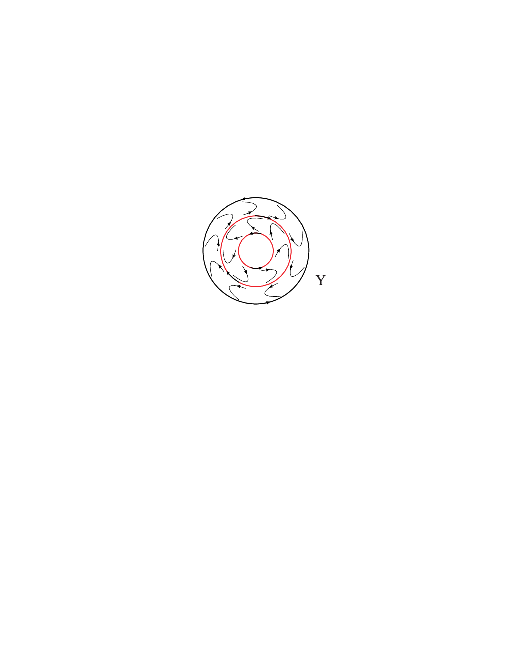
Consider the flow on the planar ring shown in Figure 1. In the polar coordinates the ring is given by the inequalities and the flow is given by the differential equations
Let , where , denote the circle . The circles are invariant under the flow. The motion along the circles and has constant angular velocity 1. Identifying any point with , we obtain a torus and a flow . The images of the circles represent two circles and on the torus . Let be a nonzero cohomology class which is the pullback of a cohomology class of . One verifies that in this example the set coincides with the whole torus . In particular, contains the periodic orbits and although clearly .
A different definition of which does not use the covering space can be found in [20].
To state the main result of this section, we need the following notion. A -cycle of the flow is defined as a pair , where and such that . If is small enough, then any -cycle determines in a canonical way a unique homology class which is represented by the flow trajectory from to followed by a “short” arc connecting with . See [20] for more details.

Theorem 5 (Farber, Kappeler, Latschev, Zehnder [21]).
Let be a smooth vector field on a smooth closed manifold . Denote by the flow generated by . Let be a cohomology class such that the restriction , viewed as a Čech cohomology class , vanishes. Then the following properties of are equivalent:
(I) There exists a smooth Lyapunov 1-form for in the cohomology class and the subset is closed.
(II) For any Riemannian metric on there exist and such that the homology class associated with an arbitrary -cycle of the flow, with , satisfies .
(III) The subset is closed and there exists a constant such that for any -invariant positive Borel measure on the asymptotic cycle satisfies
| (24) |
(IV) The subset is closed and for any -invariant positive Borel measure on with , the asymptotic cycle satisfies
| (25) |
Condition (24) can be reformulated using the notion of a quasi-regular point. Recall that is a quasi-regular point of the flow if for any continuous function the limit
| (26) |
exists. It follows from the ergodic theorem that the subset of all quasi-regular points has full measure with respect to any -invariant positive Borel measure on . From the Riesz representation theorem (see, e.g., [51], page 256) one deduces that for any quasi-regular point there exists a unique positive flow-invariant Borel measure with satisfying
| (27) |
for any continuous function . We use below the well-known fact that any positive, -invariant Borel measure with belongs to the weak∗ closure of the convex hull of the set of measures , .
If the subset is closed, and hence compact, one can apply the above-mentioned facts to the restriction of the flow to . Let be an arbitrary smooth closed 1-form lying in the cohomology class . For any quasi-regular point of the flow one has
| (28) | |||
We therefore conclude that condition (III) is equivalent to:
The subset is closed and there exists a constant such that for any quasi-regular point ,
| (29) |
where is an arbitrary closed 1-form in the class .
The value of the limit (29) is independent of the choice of a closed 1-form ; the only requirement is that lies in the cohomology class .
In the special case the set is empty and . The above statement then reduces to the following well-known theorem of C. Conley (see [5] and [55], Theorem 3.14):
Theorem 6.
(C. Conley) Let be a smooth vector field on a smooth closed manifold . Denote by the flow generated by and by the chain recurrent set of . Then there exists a smooth Lyapunov function for . This means that on and pointwise on .
We also refer to [20] where continuous Lyapunov 1-forms are studied. The paper [20] also contains a discussion comparing the results about the existence of Lyapunov 1-forms with the theorems of D. Fried [28] about the existence of cross sections for flows.
Finally we describe a class of examples of flows for which there exists a cohomology class satisfying all the conditions of Theorem 5.
Let be a closed smooth manifold with a smooth vector field . Let be the flow of . Assume that the chain recurrent set is a union of two disjoint closed sets , where . Out of this data we construct a flow on
such that , . Here denotes the de Rham cohomology class of the 1-form where denotes the angle coordinate on the circle ; is a two-point set.
We will need two vector fields and on , and . The field has two zeros corresponding to the angles and .
Let , where , be two smooth functions having disjoint supports and satisfying , .
Consider the flow determined by the vector field
Any trajectory of has the form , where , i.e., is a trajectory of . It follows that the chain recurrent set of is contained in . Over we have the vertical vector field along the circle which has two points as its chain recurrent set. Over we have the vertical vector field which has all of as the chain recurrent set. We see that , . Hence
and is closed. One easily checks that condition (III) of Theorem 5 (and hence the other conditions as well) is satisfied.
Further examples can be found in §7 of [20].
5. Notions of category with respect to a cohomology class
In this section we describe several generalizations of the classical notion of Lusternik - Schnirelmann category which reflect interesting dynamical properties of flows on manifolds. These new notions depend on a choice of a cohomology class and are all equal to the classical invariant in the case .
5.1. Movable subsets
First we define the notion of movability of a subset with respect to a closed one-form.
Definition 6.
Let be a closed one-form on a topological space . A subset is called -movable with respect to (where is an integer), if there is a homotopy such that for all , and
for all .
Note that the latter inequlaity
Below we shall think of the form being fixed and of integer being large, or tending to infinity. This may happen only in the case when the cohomology class is nonzero. Indeed, it is clear that in the case of an exact form , a nonempty subset can be -movable with respect for only for .
Any subset such that the inclusion is null-homotopic is -movable with respect to any closed 1-forms assuming that the cohomology class is nonzero.
As another example consider the following situation. Assume that is a closed smooth manifold and is a smooth closed one-form on . If has no zeros then any subset is -movable with respect to for any integer . In this case a homotopy is given by the gradient flow (appropriately scaled) of with respect to a Riemannian metric on .
In general there are topological obstructions to movability of subsets which are captured by topological invariants of Lusternik - Schnirelmann type described below.
5.2. Various notions of category
Here is the first version of the notion of a category with respect to a cohomology class. The definition given below is equivalent to the original definition of [16], see [18].
Definition 7.
Let be a finite CW-complex and . Fix a closed 1-form representing . Then the number
is defined the minimal integer such that for every there exists a closed subset which is -movable with respect to and such that .
Recall that for , is the minimal integer such that can be covered by open subsets of each of which is null-homotopic in .
Note that the number does not depend on the choice of a closed one-form and may depend only on the cohomology class . Indeed, if is another closed 1-form lying in the same cohomology then for some continuous function . Then for any path one has
Since is compact we see that there exists a constant such that for all paths in one has
Hence any subset which is -movable with respect to is -movable with respect to .
It may happen that
see Example 10.10 in [19]. Therefore it makes sense to introduce (as was suggested first in [61]) a symmetric version of which suit better dynamics applications:
Definition 8.
Let be a finite CW-complex and . Fix a closed 1-form representing . Then the number
is defined the minimal integer such that for every there exists a closed subset which is -movable with respect to both and and such that .
Clearly, one has
Reversing the quantifiers in Definition 7 gives a slightly different notion which was initially introduced in [18]:
Definition 9.
Let be a finite CW-complex and . Fix a closed 1-form representing . Then the number is defined as the minimal integer such that there exists a closed subset , which is -movable with respect to for every , and such that .
The invariant also has a symmetric modification The latter is defined similarly to with the only difference that in Definition 9 one requires that the closed subset is -movable with respect to both one-form and .
Yet another invariant similar in spirit is given by the following definition:
Definition 10.
Let be a finite CW-complex and . Fix a closed 1-form representing . Then is defined as the minimal integer such that there exists an open subset satisfying
(a) ;
(b) for some homotopy one has
for any point ;
(c) the limit in (b) is uniform in .
The symbol denotes the integral where the path is given by .
Remark 1.
The definition of given above differs from the original definition suggested in [17]; the latter was symmetric and stronger in some examples.
Independence of and of the choice of closed one-form with follows similarly to the argument given above for the case of .
The role the invariants , and play in dynamics will be discussed in the following sections.
Lemma 9.
In the case of the trivial cohomology class the numbers
coincide with the classical Lusternik - Schnirelmann category .
Proof.
We will give the proof for . If we may take and hence any subset which is -movable with respect to is empty assuming that . Hence we obtain that . ∎
Example 1.
Suppose that is a locally trivial fibration and where , . Then
| (30) |
(see [19]). Note that can be arbitrarily large in this example. Hence the new “cats” are not always equal the classical .
Comparing the definitions one trivially has
| (31) |
We will show later that may be significantly smaller than . At the moment we do not have examples when but we believe that such examples exist.
Lemma 10.
Suppose that and is connected. Then
| (32) |
The proof of this Lemma can be found in [19].
As another example consider a bouquet , where is a finite polyhedron, and assume that the class satisfies and . One can show (see [19]) that then
5.3. Homotopy invariance
Proposition 11.
Let be a homotopy equivalence between finite connected CW-complexes, and . Then
This statement remains true if one replaces by or .
Proof.
Let be a closed 1-form on representing . Let and satisfy . Because of compactness of , there exists a constant such that
for all , where . Assume that a subset is -movable with respect to the closed one-form on . Let be a homotopy such that and for all where . Then the set is -movable with respect to . Indeed, one may define a homotopy by
and for one has where .
If then for any there exists a closed subset which is -movable with respect to and such that . Then is -movable with respect to and, as is well-known, one has . This proves that .
The inverse inequality follows similarly if . The arguments for and are similar. ∎
5.4. Spaces of category zero
Here we collect some simple observations about spaces of category zero. More information can be found in [61], §3.
Lemma 12.
Let be a finite CW complex and . The following properties are equivalent:
(a) .
(b) .
(c) .
(d) There exists a continuous closed 1-form on representing (in the sense of subsection 3.3) and a homotopy , where , such that for any point one has
| (33) |
In (33) the integral is calculated along the curve , .
(e) For any continuous closed 1-form on representing there exists a homotopy , where , such that for any point inequality (33) holds.
Proof.
By Definition 7, means that the whole space is -movable for any , i.e. given , there exists a homotopy , where , such that and
| (34) |
for any . Hence, (a) implies (d).
Conversely, given property (d), using compactness of we find such that (33) can be replaced by . Now, one may iterate this deformation as follows. The -th iteration is a homotopy , where , defined as follows. Denote by the -fold composition ( times). Then for one has
| (35) |
If for any one has then for the -th iteration we obtain and (d) follows assuming that . This shows equivalence between (a) and (d).
(e) (d) is obvious. Now suppose that (d) holds for and let be another continuous closed one-form lying in the same cohomology class, i.e. where is continuous. Using compactness of we may find such that for any path one has . Fix and apply equivalence between (a) and (c) to find a homotopy with . Then one has , i.e. (e) holds.
It is obvious that (b) (a). Hence we are left to show that (a) implies (b). Given (b) fix a deformation as described in (c). Let be such that for any and for any one has . Then for any iteration (see above) one has and the result follows. ∎
In the case when is a closed smooth manifold a deformation as appearing in (b) can be constructed as the flow generated by a vector field on satisfying .
The remark of the previous paragraph explains why the following statement can be viewed as an analogue of the classical Euler - Poincaré theorem:
Theorem 7.
implies .
Proof.
Pairs with form an “ideal” in the following sense:
Lemma 13.
Let and be finite cell complexes and , . If then where
Proof.
The statement follows directly by applying the definitions. ∎
6. Focusing effect
In this section we start surveying applications of the invariant in dynamics. We describe the focusing effect discovered in [16], see also [19].
The nature of the Lusternik-Schnirelmann type theory for closed 1-forms is very much distinct from both the classical Lusternik-Schnirelmann theory for functions and from the Novikov theory. As we know, in any nonzero cohomology class , , one may always find a representing closed 1-form having at most one (highly degenerate) zero. Hence, quantitative estimates on the number of zeros may be obtained only under some additional assumptions. It turns out that these additional assumptions can be expressed in terms of some interesting dynamical properties of gradient-like vector fields for a given closed 1-form. This makes the new theory potentially very useful for dynamics.
Let be a smooth vector field on a closed smooth manifold . Recall that a homoclinic orbit of is defined as an integral trajectory ,
such that both limits and exist and are equal
More generally, a homoclinic cycle of length is a sequence of integral trajectories , of such that
for and

Homoclinic orbits were discovered by H. Poincaré and were studied by S. Smale. In the mathematical literature there are many results about existence of homoclinic orbits in Hamiltonian systems. For obvious reasons homoclinic orbits cannot exist in gradient systems for functions corresponding to the classical Lusternik-Schnirelmann theory.
One of the main theorems of this section (Theorem 8, originally established in [16]) states that any smooth closed 1-form on a smooth closed manifold must have at least geometrically distinct zeros (where denotes the cohomology class of ) assuming that admits a gradient-like vector field with no homoclinic cycles.
Viewed differently, the main result of the section claims that any gradient-like vector field of a closed 1-form has a homoclinic cycle if the number of zeros of is less than .
Definition 11.
Let be a smooth closed manifold and let be a smooth closed 1-form on with the set of zeros
We say that a smooth vector field on is a gradient-like vector field for if is a Lyapunov 1-form for the pair where is the flow on generated by the field , see Definition 5.
Note that this implies that
| (36) |
on and is invariant with respect to the flow generated by .
In the special case when the set of zeros is finite, a vector field is a gradient-like vector field for iff the sets of zeros of and of coincide and the inequality (36) holds on .
Theorem 8 (Farber [16]).
Let be a smooth closed 1-form on a closed smooth manifold . If admits a gradient-like vector field with no homoclinic cycles then has at least geometrically distinct zeros.
Here denotes the cohomology class of .
Next we give a reformulation of the above theorem:
Theorem 9.
If the number of zeros of a smooth closed 1-form is less than , then any gradient-like vector field for has a homoclinic cycle.
Note that the definition of gradient-like vector field in this paper is slightly more general than the one used in [16], [19].
A slightly more informative statement was proven in [19]:
Theorem 10 (Farber [19], Theorem 10.16).
Let be a smooth closed 1-form on a closed manifold having less than zeros, where . Then there exists an integer such that any gradient-like vector field for has a homoclinic cycle satisfying
| (37) |
One may combine these results with Theorem 4 which guarantees existence of closed 1-forms with at most one zero in any nonzero integral cohomology class. This shows that there always exist homoclinic cycles which cannot be destroyed while perturbing the gradient-like vector field!
This “focusing effect” starts when the number of zeros of a closed 1-form becomes less than the number . It is a new phenomenon, not occurring in Novikov theory. Indeed, if we assume that the zeros of are all Morse type, then (by the Kupka-Smale Theorem [58]) it is always possible to find a gradient-like vector field for such that any integral trajectory connecting two zeros comes out of a zero with higher Morse index and goes into a zero with lower Morse index; such a vector field has no homoclinic cycles.
As an illustration we will state here the following result which is a consequence of Theorem 9 and depends on a calculation of in the case when is a product of surfaces, see Theorem 25 below.
Theorem 11.
Let denote the product where each is a closed orientable surface of genus . For a cohomology class we denote by the number of indices such that . Let be a smooth closed 1-form on lying in the cohomology class and having at most zeros. Then any gradient-like vector field for has a homoclinic cycle.
Theorem 9 was generalized by J. Latschev [32] who studied a more general case of closed 1-forms having infinitely many zeros. The result of Latschev gives a “comparison” between the topology of the set of zeros of and the invariant . We prove below in §8 of this paper the following strengthening of the main Theorem of [32] and of Theorem 10:
Theorem 12.
Let be a smooth closed 1-form on a smooth closed manifold . Assume that the set of zeros admits a neighbourhood such that is exact22 2 This condition is automatically satisfied if either the cohomology class is integral or is an ENR, see Lammas 6, 7. and has finitely many connected components which satisfy
| (38) |
where denotes the cohomology class of . Then there exists an integer such that for any gradient-like vector field for there exists a finite chain of orbits
lying in (with ) and labels such that
| (39) |
for all and additionally one has
| (40) |
In other words, if the set of zeros of a closed 1-form is “small” in some sense, i.e. it satisfies the inequality (38), then any gradient-like vector field for has a generalized homoclinic cycle making at most full twists with respect to .
Note that conditions (39) describe a generalization of the notion of homoclinic cycle. Indeed, (39) intuitively means that the -th trajectory “ends” at the same connected component of from which the next -th trajectory “originates”. Such sequence of trajectories will be called a generalized homoclinic cycle.

7. Existence of flow-convex neighborhoods
In this section we study some auxiliary problem which will be used in the proof of Theorems 12 and Theorem 14 and is also of independent interest. The results of this section are typical for the Conley theory of isolated invariant sets. We follow here the paper [18].
Consider a smooth vector field on a closed smooth manifold . Let be the flow of . We will write as , where and . The symbol denotes the chain recurrent set of .
Theorem 13 (Farber - Kappeler [18]).
Let be a connected component of which is isolated in , i.e. such that there exists a neighborhood with . Let be a neighborhood of . Then there exists an open neighborhood of , contained in , with the following two properties:
(A) For any , the open set
is convex (i.e. it is either empty or an interval);
(B) Let be the set of points such that the interval is nonempty and bounded below. Then the function
is continuous.
A neighborhood of having properties (A) and (B) is called convex with respect to the flow .
By Conley’s theorem [5, 6], there exists a smooth Lyapunov function for the flow; see also [21], Proposition 2, where the proof of the smooth version of Conley’s theorem is given. The Lyapunov function satisfies: on the complement of and the differential vanishes on .
Fix a point and consider its orbit . The function is strictly decreasing. Hence, as tends to the limit
| (41) |
exists and is finite. If then the function is constant.
![[Uncaptioned image]](0807.3240v2/ell.png)
For any the number is a critical value of . Indeed, the -limit set is contained in the level set and, on the other hand, is a part of the chain recurrent set which is the set of critical points of .
Lemma 14.
The function is upper semi-continuous: if then
| (42) |
Proof.
Given any there exists such that . Since is continuous and the map is continuous, there exists a neighborhood of such that for any . Hence for all one has
Hence, . ∎
The function restricted to is constant. Indeed, must be connected (as the image of a connected set) and it has measure zero by Sard’s theorem. Hence it is a single point. Denote .
Let be an open neighborhood. As is supposed to be isolated in , we may assume (without loss of generality) that .
Fix and denote by the set of all points with the properties: (a) ; (b) . Note that (b) implies that .
Lemma 15.
For any sufficiently small the set is contained in the neighborhood .
Proof.
Assuming the contrary, there exists a convergent sequence such that and , and , where denotes the -limit set of the trajectory . If is the limit of then (using (42)) one has . On the other hand, and hence . We obtain that belongs to the set In other words, it lies in a connected component of distinct from .
Fix a Riemannian metric on . Denote by the distance between and . Denote by a constant such that the norm of the vector is less than at every point of . Such exists since is compact.
Fix some such that . The function restricted to the complement of the -neighborhood of is negative and moreover can be estimated from above for some positive . Now, we may find a large such that
and lies in the -neighborhood of . The trajectory approaches for large . The length of the trajectory is given by
One concludes that the time the trajectory for spends in the complement of the -neighborhood of can be estimated by
Therefore, for large one has
These inequalities show (since tends to ) that for large one has contradicting the assumption . ∎
Remark 2.
Define as the set of all points with and where denotes the -limit set of the trajectory . Applying the above arguments to the time reversed flow one obtains that for any neighborhood of the set is contained in for any sufficiently small .
The arguments of the proof could be summarized as follows: the point is very close to a component of lying in and distinct from . The trajectory starting at cannot approach since while it passes the distance separating and it descends with respect to so that the point slips below the level .
Lemma 16.
For any sufficiently small the set is closed.
Proof.
Let be a neighborhood of with and let be such that . Assume that a sequence converges to a point . Then, for any the point lies in . Hence we obtain that for any the point lies in . It follows that . Hence, is an element of . ∎
Lemma 17.
Let be an open neighborhood of such that . Let be such that is contained in for any . Then there exists an open neighborhood of the set in the level set and an open neighborhood of in with the following properties:
- (1)
If then for some the point lies in .
- (2)
The mapping is a homeomorphism of .
- (3)
For any the point lies in .
- (4)
The number depends continuously on and it tends to as approaches .
![[Uncaptioned image]](0807.3240v2/boxik1.png)
Proof.
If and is close enough to the set then for the orbit does not leave before it leaves the set . Indeed, if this claim is false then there exists a sequence of points and a sequence of numbers such that , , , and . Fix a Riemannian metric on . Let be such that the length of the vector is less or equal than at every point . Choose a small neighborhood of such that its closure is contained in . Let be the distance between and . The function satisfies in the inequality for some . Now, let be a neighborhood of such that
As belongs to there exists with . Then for large enough . Arguing as in the proof of Lemma 15, one obtains that the point cannot reach before it leaves the domain .
Similarly we observe: if where is sufficiently close to then the trajectory for some reaches the level without leaving . Indeed, if this statement is false one finds a sequence , such that and for some , , . We may assume that the sequence converges to a point . If the forward trajectory where crosses the level surface at a point which is not in and the trajectory must cross this level at a nearby point as , a contradiction. Hence we have to consider only the case which leaves two possibilities: either is contained in a connected component of distinct from which also lies on the level surface , or . The first possibility leads to a contradiction, arguing as in the proof of Lemma 15. The second possibility means that belongs to where . This is a contradiction since we assume that is contained in the open set .
Let be the union of the set and the set of all points such that the trajectory for reaches the set without leaving .
Let be the union of and the set of all such that the trajectory for reaches the level surface without leaving .
is an open neighborhood of in and is an open neighborhood of in as was shown above. It is then easy to see that the statements of Lemma 17 hold for and . Let us show, for example, that if and then tends to . If not one may pass to a subsequence such that the sequence has a finite limit . Then . Thus the trajectory arrives in finite time at which is impossible since is flow-invariant and . ∎
Here is an analog of Lemma 17:
Lemma 18.
Let be an open neighborhood of such that . Let be such that is contained in for any . Then there exists an open neighborhood of the set in the level set and an open neighborhood of in with the following properties:
- (1)
If then for some the point lies in .
- (2)
The mapping is a homeomorphism
- (3)
For any the point lies in .
- (4)
The number depends continuously on and it tends to as approaches .
Proof.
It is similar to the proof of Lemma 17. ∎
Proof of Theorem 13.
Let be an open neighborhood of . We may assume without loss of generality that . By Lemma 15 and Remark 2 we may find such that for any the sets and are contained in .
Let denote the set of all points such that there exist numbers with
| (43) |
and is contained in for any . Observe that if then is contained in .
Define the set
We are going to show that it satisfies the requirements of Theorem 13. This set is open. Indeed, the terms in (43) are pairwise disjoint. The set is clearly open. Any point of (where ) has a neighborhood contained entirely in (by Lemmas 17 and 18). Similarly, any sufficiently small neighborhood of a point is contained in : if and then the trajectory for either approaches (in that case lies in for some ) or it hits the level surface . In the second case the intersection point is very close to and hence by Lemmas 17 and 18 the trajectory continues all the way till it reaches the level without leaving .
Given consider the set . Let us assume that . Then there exist the following possibilities:
- (1)
; then .
- (2)
; then is a half infinite interval .
- (3)
and ; then .
- (4)
; then is either the empty set or a finite interval .
In the case the arguments are similar.
The continuity of follows from the Implicit Function Theorem: the number is the solution of the equation and the partial derivative of with respect to is strictly negative. ∎
8. Proof of Theorem 12
The arguments are similar to those use in the proof of Theorem 4.1 of [16].
Suppose that Theorem 12 is false, i.e. for any there exists a gradient-like vector field for having no generalized homoclinic cycles of integral trajectories satisfying (39) and (40). Our goal is to show that then
| (44) |
i.e. the inequality (38) is violated. Without loss of generality we may assume that the number of connected components is finite since if the inequality (44) is obviously true, as for any .
Fix a Riemannian metric on . We will denote the flow generated by by , where and . Since on , the integral is non-positive and non-increasing for .
We start by proving the following Lemma:
Lemma 19.
Assume that for an integer there exists a gradient-like vector field for having no generalized homoclinic cycles of integral trajectories satisfying (39) and (40). Let be an open neighbourhood of , where . Then there exists a family of smaller closed neighbourhoods of satisfying the following properties:
- (a)
Each set lifts to the covering space corresponding to the kernel of the homomorphism of periods determined by the cohomology class .
- (b)
The lift of into is flow convex (i.e. it satisfies properties (A) and (B) of Theorem 13) with respect to the natural lift of the flow into .
- (c)
Let denote the exit set of , i.e. the set of all points such that for all sufficiently small one has . Then there exist no and such that and .
The intuitive meaning of property (c) is that it is impossible for a trajectory to leave and then revisit in time without making the quantity smaller than .
![[Uncaptioned image]](0807.3240v2/return.png)
Proof.
Without loss of generality we may assume that the initial neighbourhoods satisfy properties (a) and (b) of Lemma 19.
Let be any closed neighborhood of satisfying (b); then (a) is automatically satisfied. Denote by and the unions , and . We claim:
- (i)
There exists such that for any and with one has .
Indeed, as follows from the gradient convexity of the sets , any trajectory starting at at leaves before it can re-enter . Hence, we may take , where denotes the distance between and , and for .
Note that if we shrink the sets , the number may only increase, assuming that are sufficiently small.
- (ii)
There exists such that for any and with one has
Indeed, we may take
From (i) and (ii) it follows that:
- (iii)
There exists an integer such that for any the set
is a union of at most disjoint intervals, i.e.
and
Indeed, the number of gaps between the intervals is at most as follows from (ii).
For a point we denote by
| (45) |
the backward and forward limit sets of the trajectory passing through . These sets are nonempty, compact, connected and flow-invariant.
Now, suppose that we can never achieve (c) by shrinking the initially chosen neighbourhoods . We want to show that then there exists a sequence of points and an injection such that
where and and additionally the following inequality is satisfied
| (46) |
where the curve is given by for which would contradict our assumptions.
There exists an infinite sequence of points , where , and two sequences of real numbers and such that
- (1)
the set is contained in a fixed connected component and the distance tends to as ;
- (2)
converges to as ;
- (3)
one has
(47)
Passing to a subsequence, we may assume that converges to a point and the sequences and have finite or infinite limits, which we denote by and respectively. Because of property (iii), we may also assume that the number of intervals is independent of and the sequences and have finite or infinite limits denoted by and respectively for . Moreover, for the same reasons, we may assume that as the sequences
converge to points correspondingly, where .
It is easy to see that (1) and (2) imply that and .
Note that . Indeed, by (1), one has and therefore the set must be contained in the maximal invariant subsets of .
s
![[Uncaptioned image]](0807.3240v2/catch5.png)
Clearly the points lie on the boundary of the same connected component of where is a map and . The points and either lie on the same orbit of the flow or one has
| (48) |
as follows from arguments mentioned above. We may ignore the first case since then we may simply relabel the points and apply the following observations. The points and lie on the same orbit and hence we may rewrite (48) in the form
| (49) |
where . For the last point we have
Hence we obtaine a closed chain of integral trajectories – a generalized homoclinic cycle. Inequality (46) follows from (47) by passing to the limit and observing that the form is exact, where is smooth. Moreover the function is constant on . Indeed, the image is connected and has measure zero by Sard’s theorem; hence is a single point. These remarks imply that
for any .
This completes the proof of Lemma 19. ∎
Proof of Theorem 12.
Assume that under the condition of Theorem 12 there exist no generalized homoclinic cycles satisfying (40). Applying Lemma 19 with neighbourhoods such that we obtain a system of neighbourhoods satisfying (a)-(c) of Lemma 19 and also where .
Define sets as follows. We say that if for some the point belongs to the interior of , and
It is clear that is open.
Let us show that can be deformed into . For any point let denote the set . Because of our assumption about the gradient-convexity of neighborhood , the set is a union of disjoint closed intervals, and some of these intervals may degenerate to a point. Consider the first interval . If this interval degenerates to a point (i.e., the trajectory through touches ), then does not belong to the set , according to our assumption (c); see above. For the same reason, points of do not belong to .
Assume now that and . Then the point lies in the interior of for . Also, we have
The function , given by
is continuous since . One may now define a homotopy
Here is the inclusion and maps into the interior of . By Lemma 19.5 from [8] we obtain
and therefore
| (50) |
Consider now the complement . For any point there exists such that . It is clear that is a continuous real valued function on . One may define a homotopy
Then for any one has
i.e. the closed set is -movable with respect to and
9. Topology of the chain recurrent set
In this section we prove the following result from [18].
Theorem 14 (Farber - Kappeler).
Consider a smooth flow on a closed smooth manifold . Let be a cohomology class such that the following conditions are satisfied:
(1) The chain recurrent set is isolated in the full chain recurrent set of .
(2) The restriction
(viewed as a Čech cohomology class) vanishes.
(3) For any -invariant, positive Borel measure on with , Schwartzman’s asymptotic cycle satisfies
Then one has the following inequality
| (51) |
where denote the connected components33 3 The number of connected components of can be infinite. In this case inequality (14) is trivially satisfied as its LHS is infinite. of the chain recurrent set .
Let us compare Theorem 14 with Theorem 6.6 of [17]. Theorem 14 allows arbitrary sets whereas Theorem 6.6 of [17] assumes that consists of finitely many isolated points. Another important advantage of Theorem 14 is that it does not require condition (), see [17], page 108; this condition is difficult to check in concrete examples. On the other hand, since , the estimate of Theorem 6.6 of [17] is potentially slightly sharper.
Next we state some corollaries of Theorem 14.
In the special case one has and the assumptions (1), (2), (3) of Theorem 14 are automatically satisfied. Hence we obtain the following result which presumably is well known but for which we failed to find a reference:
Theorem 15.
Consider a smooth flow on a closed smooth manifold . Let be the chain recurrent set of the flow. Then
| (52) |
Here denote the connected components of .
In the special case where the chain recurrent set consists of finitely many points (the fixed points of the flow) Theorem 15 says that the number of fixed points is at least the Lusternik - Schnirelman category of . This is one of the fundamental results of the classical Lusternik – Schnirelman theory, see [8].
Consider another special case of Theorem 14 when consists of finitely many points (they are the fixed points of the flow). Condition (2) of Theorem 14 is automatically satisfied under these assumptions. We obtain:
Theorem 16 (Farber - Kappeler).
Consider a smooth flow on a closed smooth manifold . Let be a cohomology class such that the chain recurrent set consists of finitely many points which are isolated in the full chain recurrent set of the flow. Assume additionally that condition (3) of Theorem 14 is satisfied. Then the flow has at least fixed points.
Here is a reformulation of Theorem 16:
Theorem 17 (Farber - Kappeler).
Let be a cohomology class. Consider a flow on such that the chain recurrent set consists of less than fixed points and such that condition (3) of Theorem 14 is satisfied. Then at least one of the fixed points of the flow is not isolated in the full chain recurrent set .
Here is a typical application of Theorem 16:
Theorem 18 (Farber - Kappeler).
Let be a smooth flow on a closed smooth manifold such that the chain recurrent set of is a union of finitely many circles and isolated points. Let be a cohomology class such that for the homology class of any periodic orbit. Then
| (53) |
where denotes the number of fixed points of the flow, denotes the number of periodic orbits which are null-homotopic in , and denotes the number of periodic orbits which are homotopically nontrivial but their homology classes satisfy .
Proof.
In the special case of Theorem 18 condition (3) of Theorem 14 is equivalent to the requirement that for the homology class of any periodic orbit. Under the assumptions of Theorem 18 the set is the union of the fixed points and of the periodic orbits satisfying . If is a periodic orbit then the number equals 1 or 2 depending on whether is or is not null-homotopic in . These consideration show that Theorem 18 follows from Theorem 14. ∎
10. Proof of Theorem 14
Consider a smooth flow , and a real cohomology class satisfying the conditions of Theorem 14.
If the chain recurrent set has infinitely many connected components then the RHS of inequality (51) is infinite and so this inequality is obviously satisfied. Hence without loss of generality we may assume that the number of connected components of is finite.
Let be the connected components of . Fix mutually disjoint open neighborhoods , where . We shall assume that is so small that
| (55) |
Compare [8], Lemmas 19.2 and 19.6.
Applying Theorem 13 we may find an open neighborhood of which is convex with respect to the flow . Clearly,
| (56) |
as a consequence of (55).
Let be an open neighborhood of such that the closure is contained in . We have the inclusions .
Let denote the set of points such that for any the point does not belong to the union . The set is closed and flow-invariant.
Applying Theorem 5 we find that there exists a smooth Lyapunov 1-form for the pair lying in the cohomology class . This means that the function is negative on (where denotes the vector field on generating the flow ) and . Moreover, the restriction of on some open neighborhood of is the differential of a smooth function (this is equivalent to condition (1) of Theorem 14).
Let us show that for any integer the set is -movable with respect to both and . Since is compact there exists such that on . Then for any one has
Hence a continuous homotopy , defined by
satisfies the condition of Definition 6. This shows that is -movable with respect to . In a similar way one shows that for any integer the set is -movable with respect to .
Let denote the set of points such that belongs to for some . Then is a nonempty open interval. For define
The function is continuous as follows from Theorem 13.
11. Cohomological estimates for
The effectiveness of dynamical applications described in sections §§6 - 10 depend crucially on the ability to calculate, or to estimate from below, the quantity where is a finite polyhedron and is a cohomology class. The situation here is quite similar to the classical Lusternik - Schnirelmann theory where is most often computed by a combination of upper and lower bounds and the most popular lower bound for uses the cohomological cup-length, see [8].
In this section we discuss results of this type for following our paper [25]; some lower bounds for were obtained earlier in the papers [16] and [19]. We give in this section the main definitions, state principal results and illustrate them by several specific examples; however for complete proofs we refer the reader to our original papers [25], [26] and [24].
Let be a finite polyhedron and . Denote by the kernel of the homomorphism given by evaluation on . Then is a free abelian group of finite rank where denotes the rank of class . Consider the cover corresponding to . It has as the group of covering translations.
Let denote the variety of all complex flat line bundles over such that the induced flat line bundle on is trivial. If is a basis, then the monodromy of along is a nonzero complex number and the numbers form a coordinate system on . Given a flat line bundle the monodromy representation of is the ring homomorphism
| (58) |
sending each to . The dual bundle is such that is trivial; if are coordinates of then are coordinates of .
Any nontrivial element lying in the kernel of can be viewed as a (Laurent) polynomial equation between the variables . Alternatively, we will consider algebraic subvarieties . Any such is the set of all solutions of a system of equations of the form
where is a Laurent polynomial with complex coefficients
This is equivalent to fixing an ideal and studying the set of all flat line bundles such that
Definition 12.
(1) We say that a bundle is -algebraic if the monodromy homomorphism has nontrivial kernel.
(2) We say that is a -algebraic integer if the kernel of contains a nontrivial polynomial with -top coefficient (see below).
(3) We say that is -transcendental if is injective.
Any nonzero can be written as where , , and The nonzero integer is called the -top coefficients of .
If is a basis and if denotes the monodromy of along , i.e. , then is -algebraic iff there exist a nontrivial Laurent polynomial equation with integral coefficients such that .
There exist countably many nonzero Laurent polynomials with integral coefficients and for each such the set of solutions is nowhere dense in . Since is homeomorphic to a complete metric space we obtain:
Lemma 20.
The set of all -transcendental bundles is of Baire category 2. In particular, the set of -transcendental is dense in the variety .
Lemma 21.
For any -transcendental flat line bundle the dimension of the vector space equals the -dimensional Novikov - Betti number ,
Proof.
The monodromy homomorphism defines a left -module structure on and by definition
| (59) |
where is the cellular chain complex of the covering corresponding to . If is transcendental then gives a field extension where is the field of fractions of . We obtain therefore (using finiteness of over and (59)):
This implies that for any transcendental one has
| (60) |
and the right hand side. Finally we invoke Proposition 1.30 of [19] which explains why the right hand side of (60) equals the Novikov - Betti number . ∎
Theorem 19 (Farber - Schütz, [25]).
Let be a finite cell complex and . Let be -transcendental. Assume that there exist cohomology classes and where such that for and the cup-product
| (61) |
is nontrivial. Then .
Theorem 19 combines simplicity with remarkable efficiency. Below in this section we test this theorem in many specific examples.
11.1. The notion of cup-length
In view of Theorem 19 we introduce the following notation.
Let be a finite cell complex and . We denote by the maximal integer such that Theorem 19 could be applied to ; if Theorem 19 is not applicable (i.e. if for any -transcendental , compare Lemma 21) we set
Hence,
| (62) |
In other words, where iff there exists a -transcendental flat line bundle and there exist cohomology classes and where and for such that the cup-product
| (63) |
is nontrivial.
Note that for the number coincides with the usual cup-length ; recall that the later is defined as the largest integer such that there exist cohomology classes where of positive degree such that their cup-product is nontrivial.
One can restate Theorem 19 as follows:
Theorem 20.
For any finite complex and one has
The next useful Lemma suggests several different ways to characterize the number . This Lemma plays an important role in the sequel.
Lemma 22.
Let be a finite cell complex and . The following statements regarding an integer are equivalent:
- (A)
;
- (B)
There exists cohomology class where is a -transcendental flat line bundle and there exist integral cohomology classes where and for , such that the cup-product (63) is nontrivial.
- (C)
Let denote and let denote the field of fractions of the group ring . Then there exist cohomology classes and where for such that the cup-product
is nontrivial.
- (D)
For any -transcendental flat line bundle there exists cohomology class such that the cup-product (63) is nontrivial for some integral cohomology classes with for .
- (E)
For any -transcendental flat line bundle there exist cohomology classes and where and for such that the cup-product (63) is nontrivial.
Proof.
Let us show that (A)(B). Fix a -transcendental bundle , and such that (63) is nontrivial for some with . Consider now the cup-products
| (64) |
with arbitrary integral cohomology classes ; here the degrees are assumed to be fixed. (64) is a multi-linear function of the classes . Since the integral classes generate over we obtain that (64) must be nonzero for some choice of classes , i.e. (B) holds.
Now we show that (B)(C). Fix and the classes and satisfying conditions described in (B). The monodromy homomorphism is an injective ring homomorphism, it extends to the field of fractions . The image of the induced homomorphism on cohomology
| (65) |
generates over and (65) is injective (for reasons mentioned in the proof of Lemma 21). Fix cohomology classes where . For a cohomology class the function
| (66) |
extends to a -linear function of
If this function is nonzero then it may not vanish on the image of , i.e. (C) holds.
Implications (D)(E) and (E)(A) are obvious. This completes the proof. ∎
Lemma 23.
Assume that and are path connected finite cell complexes and . Then
| (67) |
Proof.
Denote and . Any flat line bundle over has the form (exterior tensor product) where and are flat line bundles over and respectively. Note that if lies in the variety then and are obtained by restrictions and hence and . We will use equivalence between (A) and (E) of Lemma 22. Fix a -transcendental bundle over . Then both and are -transcendental. Find classes , , , such that and . Now we have cohomology classes and and the product
is nonzero. Here we use the Künneth formula which states
| (68) |
This proves (67). ∎
11.2. Some examples
In this section we apply Theorem 19 in a few simple examples.
11.2.1.
First consider the case . We know that for the number coincides with the classical LS category , see [19], Example 10.8. Let us examine what Theorem 19 gives in this case. The variety has only one point – the trivial flat line bundle over . The support is always empty for . We may therefore take applying Theorem 19. Thus, we see that Theorem 19 claims in the special case that if there exist cohomology classes with then . This claim is the classical cup-length estimate for the LS category .
11.2.2.
Note that if and is connected then for any nontrivial . Note also that the trivial flat line bundle is never -transcendental. Therefore the degree of the class (which appears in Theorem 19) in the case must be positive. Hence for the number in Theorem 19 satisfies . This explains why Theorem 19 cannot give for .
Lemma 10 yields
| (69) |
assuming that is connected and . This is consistent with the remark of the previous paragraph.
11.2.3.
The following example shows that (69) can be satisfied as an equality i.e. that is possible. Consider the bouquet where is a finite polyhedron, and assume that the class satisfies and We know that in this case
| (70) |
see Example 10.11 from [19].
We are going to apply Theorem 19. The variety in this case coincides with the set The support contains in this case only the trivial line bundle. is -transcendental if the monodromy along the circle is a -transcendental complex number. For any the restriction is trivial and the restriction homomorphism is onto.
Suppose that the cohomological cup-length of with -coefficients equals , i.e. there exist cohomology classes of positive degree such that the product is nonzero. By the above remark, for a nontrivial we obtain cohomology classes and such that . Hence . By Theorem 19 we obtain which is equivalent (taking into account (70)) to . The last inequality is the classical cup-length estimate for the usual category.
11.2.4.
Let us now consider a very specific example: . In this case and we describe as function of . We denote by the set of all classes such that . Clearly is a line through the origin in . We claim that:
Indeed, consider first the case , i.e. . Let us show that . Denote and let be a point distinct from . Set and . Then is an open cover of with null-homotopic and with being -movable in for any (assuming that ; this follows from homotopy invariance of and from Example 1.
Since would imply by Theorem 7 stated below we obtain that for any (as ). This proves the first line of (11.2.4).
If we apply (70) to obtain .
For we easily find .
12. Upper bounds for and relations with the Bieri - Neumann - Strebel invariants
Bieri, Neumann and Strebel introduced in [2] a geometric invariant of discrete groups which captures information about the finite generation of kernels of abelian quotients of . In this section we describe a relation between this invariant and properties of .
Let us recall the definition. We always assume that is finitely presented as this is sufficient for our purposes. Let denote where acts on by multiplication. Clearly is a sphere of dimension where is the rank of the abelianization of . Denote by the equivalence class of a nonzero homomorphism . The Bieri-Neumann-Strebel invariant associates to a subset defined as follows44 4 We rely on Theorem 5.1 of [2] which states that the definition of given above coincides in the case of finitely presented with the main definition of [2].. Let be a finite cell complex with and let be the universal abelian cover of . A homomorphism can be viewed as a cohomology class lying in . One has if and only if the inclusion induces an epimorphism where is a connected neighborhood of infinity with respect to , see §2 of [25] and Lemma 5.2 from [2].
The following Theorem summarizes the results proven in [25]:
Theorem 21 (Farber - Schütz).
- (a)
Let be a finite connected polyhedron and let be nonzero. Then
- (b)
Let be a closed connected smooth manifold and let be nonzero. Then
- (c)
Let be a closed connected smooth manifold of dimension and let be nonzero. If either
then
- (d)
Let be a closed connected smooth manifold of dimension and let be nonzero. If both inclusions take place
then
13. Homological category weights, estimates for and calculation of , for products of surfaces
In this section we describe briefly the results obtained in [26] which has as its main goal obtaining cohomological lower estimates for . In particular we will see that there are many examples when and the difference can be arbitrarily large.
The first step is the introduction of a new notion of category weight of homology classes which is somewhat dual to the cohomological notion introduced by E. Fadell and S. Husseini [9]. It was a pleasant surprise to discover that the homological category weight is homotopy invariant unlike the cohomological version of Fadell and Husseini.
The notion of homological category weight allows us to obtain improved cohomological lower bounds for .
13.1. Homological category weight
The classical cohomological lower bound for the Lusternik - Schnirelmann category states that if there exist cohomology classes of positive degree where , such that their cup-product is nontrivial. Here denotes a local coefficient system on and is the tensor product .
E. Fadell and S. Husseini [9] improved this estimate by introducing the notion of a category weight of a cohomology class .
Definition 13 (Fadell - Husseini, [9]).
Let be a nonzero cohomology class where is a local coefficient system on . One says that (where is an integer) if for any closed subset with one has .
Recall that the inequality means that can be covered by open subsets such that each inclusion is null-homotopic, .
According to Definition 13 one has in general and for any nonzero cohomology class of positive degree. As Fadell and Husseini [9] showed, in some special situations which improves the lower estimate for . Indeed, one has
assuming that the cup-product is nonzero.
Y. Rudyak [52] and J. Strom [60] studied a modification of , called the strict category weight . The latter has the advantage of being homotopy invariant. However in some examples the strict category weight is considerably smaller than the original category weight of Fadell and Husseini.
In [26] we introduced and exploited a “dual” notion of category weight of homology classes. It has the geometric simplicity and clarity of category weight as defined by Fadell and Husseini and has a surprising advantage of being homotopy invariant.
Definition 14 (Farber - Schütz, [26]).
Let be a singular homology class with coefficients in a local system and let be a nonnegative integer. We say that if for any closed subset with there exists a singular cycle in representing . We say that iff and .
In other words, is equivalent to the fact that can be realized by a singular cycle avoiding any closed subset with .
For example, iff can be realized by a singular cycle avoiding any closed subset such that the inclusion is homotopic to a constant map.
It will be convenient to define the category weight of the zero homology class as .
Formally if lies in the intersection
where runs over all closed subsets with .
The relation means that there exists a closed subset with such that any geometric realization of intersects . In particular we obtain the following inequality
| (75) |
for any nonzero homology class , . The last inequality can be also rewritten as
| (76) |
for any nonzero homology class.
Note that if is path-connected and is zero-dimensional, i.e. , then .
Lemma 24.
Assume that is a simplicial polyhedron. Then iff can be realized in for any sub-polyhedron with .
Proof.
We only need to show the ’if’-direction. Let be closed with . We need to show that can be realized by a cycle in . We have with each open and null-homotopic in . Passing to a fine subdivision of , we can find a sub-polyhedron with . Then and can be realized by a cycle lying in . ∎
Example 2.
Assume that is a closed 2-dimensional manifold, i.e. a compact surface. Let us show that any nonzero homology class has . Indeed, it is easy to see that any closed subset which is null-homotopic in lies in the interior of a disk ; but is an isomorphism.
Theorem 22 (Farber - Schütz, [26]).
If is a homotopy equivalence then for any homology class one has
| (77) |
Here where is the local coefficient system over induced by the homotopy inverse of .
Another important result from [26] shows how one may use the notion of homological category weight in conjunction with the notion of Fadell and Husseini to estimate :
Corollary 25.
Suppose that is a metric space and for some classes and the evaluation
is nonzero. Then
| (78) |
Here is the category weight of homology class as defined above and is the category weight of as defined by Fadell and Husseini [9].
The main idea standing behind this Corollary is that “the degree of nontriviality”of a cohomology class can be “measured” by “quality” of the homology class satisfying .
It is curious to observe that in the case of closed manifolds our notion of category weight of homology classes coincides with the cohomological notion of Fadell and Husseini [9] via the Poincarè duality. However for Poincaré complexes these notions are distinct as we show by an example given below.
Theorem 23 (Farber - Schütz, [26]).
Suppose that is a closed -dimensional manifold, where is a local coefficient system. Let be the Poincaré dual cohomology class, i.e. , see below. Then
| (79) |
Here denotes the orientation local system on , i.e. for a point the stalk of at is , see [59].
Example 3.
Let be the real projective space. For the unique nonzero cohomology class one has Indeed, the dual homology class is where is the generator. Clearly, .
Theorem 23 implies:
Corollary 26.
If is a closed -dimensional manifold then for any homology class with one has
| (80) |
Indeed, if then the dual cohomology class has positive degree and hence .
Consider now the case when is -dimensional Poincaré complex. The following example shows that Theorem 23 is false for Poincaré complexes. It is a modification of an argument due to D. Puppe showing that the notion of category weight of cohomology classes is not homotopy invariant.
Example 4.
Consider the lens space where is an odd prime and acts freely on . Denote by the quotient map. Let be the mapping cylinder of , i.e.
where each point is identified with . Clearly is homotopy equivalent to and so it is a Poincaré complex. By a theorem of Krasnoselski [30], the category of equals . Hence for one has
see above. The dual cohomology class is the generator . Let us show that
Indeed, consider the sphere . The restriction coincides with the induced class where is the generator. Hence the cohomology class is nonzero. However, the sphere has category 2 and moreover (as the inclusion is not null-homotopic).
13.2. Cohomological estimate for
The following Theorem is the main result established in [26].
Theorem 24 (Farber - Schütz, [26]).
Let be a finite cell complex and . Let be a complex flat line bundle over which is not a -algebraic integer (see Definition 12). Suppose that for an integral homology class and some cohomology classes and , where for , the evaluation is nonzero. Here , . Then one has
| (81) |
Here denotes the category weight of viewed as a homology class of with local coefficient system where is a free abelian group which can be identified with the group of periods of .
13.3. and for products of surfaces
Theorem 25 (Farber - Schütz [25, 26]).
Let denote the product
where each is a closed orientable surface of genus . Given a cohomology class , one has
| (82) |
and
| (83) |
where denotes the number of indices such that the cohomology class vanishes. In particular
| (84) |
and
| (85) |
assuming that for any .
Theorem 25 demonstrates that the difference between two notions of category with respect to a cohomology class
can be arbitrarily large.
References
- [2] R. Bieri, W. Neumann, R. Strebel, A geometric invariant of discrete groups, Invent. Math. 90 (1987), 451-477.
- [3] R. Bieri, B. Renz, Valuations on free resolutions and higher geometric invariants of groups, Comment. Math. Helv. 63 (1988), 464-497.
- [4] P. M. Cohn, Free rings and their relations, Academic Press, London, 1985.
- [5] C. Conley, Isolated invariant sets and the Morse index, CBMS Regional Conference Series in Mathematics, no. 38, AMS, 1976.
- [6] C. Conley, The gradient structure of a flow: I, Ergod. Th. & Dynam. Sys., 8(1988), 11–26.
- [7] A. Dold, Lectures on Algebraic topology, Springer-Verlag, 1972.
- [8] B. Dubrovin, S. Novikov and A. Fomenko, Modern Geometry; Methods of the homology theory, 1984.
- [9] E. Faddell, S. Husseini, Category weight and Steenrod operations, Boletín de la Sociedad Mathemática Mexicana, 37(1992), 151-161
- [10] H. Fan, J. Jost, Novikov-Morse theory for dynamical systems. Calc. Var. Partial Differential Equations 17 (2003), no. 1, 29–73.
- [11] H. Fan, J. Jost, Conley index theory and Novikov-Morse theory. Pure Appl. Math. Q. 1 (2005), no. 4, part 3, 939–971.
- [12] M. Farber, Exactness of Novikov inequalities, Functional Analysis and its Applications 19(1985), 40-48.
- [13] M. Farber and A. Ranicki, The Morse-Novikov theory of circle-valued functions and noncommutative localization, Proceedings of the Steklov Institute of Mathematics, 225(1999), pp. 363 - 371.
- [14] M. Farber, Morse-Novikov critical point theory, Cohn localization and Dirichlet units, Communications in Contemporary Mathematics, 1(1999), 467 - 495.
- [15] M. Farber, Counting zeros of closed 1-forms, “Topology, Ergodic Theory, Real Algebraic Geometry. Rokhlin’s Memorial”, V. Turaev, A. Vershik editors, Amer. Math. Translations, Ser. 2, 202(2001), 95 - 107.
- [16] M. Farber, Zeros of closed 1-forms, homoclinic orbits and Lusternik-Schnirelman theory, Topol. Methods Nonlinear Anal. 19 (2002), 123-152.
- [17] M. Farber, Lusternik-Schnirelman theory and dynamics, ”Lusternik-Schnirelmann Category and Related Topics”, O. Cornea, G. Lupton, J. Oprea and D. Tanré editors, Contemporary Mathematics, 316(2002), 95 - 111.
- [18] M. Farber, T. Kappeler, Lusternik-Schnirelmann theory and dynamics, II, Proc. Steklov Inst. Math. 2004, no. 4 (247), 232–245.
- [19] M. Farber, Topology of closed one-forms, Mathematical Surveys and Monographs, AMS, 2004.
- [20] M. Farber, T. Kappeler, J. Latschev, E. Zehnder, Lyapunov 1-forms for flows, “Ergodic theory and dynamical systems”, 24(2004), 1451-1475.
- [21] M. Farber, T. Kappeler, J. Latschev, E. Zehnder, Smooth Lyapunov 1-forms, “L’Enseignement Mathematique”, 50 (2004), no. 1-2, 3–17.
- [22] M. Farber and D. Schütz, Novikov Betti numbers and the fundamental group, Russian Math. Surveys 61 (2006), no. 6, pp. 1173–1175.
- [23] M. Farber, D. Schütz, Closed 1-forms with at most one zero, Topology, 45(2006), 465-473.
- [24] M. Farber, D. Schütz, Moving homology classes to infinity, Forum Math. 19 (2007), 281-296.
- [25] M. Farber, D. Schütz, Cohomological estimates for , Geom. Top. 11 (2007), 1255-1289.
- [26] M. Farber, D. Schütz, Homological category weights and estimates for , J. Eur. Math. Soc. 10 (2008), 243-266.
- [27] M. Farber, R. Geoghegan and D. Schütz, Closed 1-forms in topology and geometric group theory, preprint.
- [28] D. Fried, The geometry of cross sections to flows, Topology, 21(1982), 353–371.
- [29] H. Hofer and D. Salamon, Floer homology and Novikov rings, Floer memorial volume, Birkhäuser (1995), pp. 483-524.
- [30] M.A. Krasnoselski, On special coverings of finite dimensional sphere, Doklady AN SSSR, 103(1955), 961-964.
- [31] S. Lang, Real and Functional Analysis, third edition, Graduate Texts in Mathematics, 142, 1993, Springer-Verlag
- [32] J. Latschev, Flows with Lyapunov 1-forms and a generalization of Farber’s Theorem on homoclinic cycles, “International Mathematical Research Notices”, 2004:5, pp. 239-247.
- [33] J. Latschev, Closed forms transverse to singular foliations, Manuscripta Math. 121 (2006), no. 3, 293–315.
- [34] J. Latschev, Coherent measures and the existence of smooth Lyapunov 1-forms for flows, Topology 45 (2006), no. 4, 707–723.
- [35] F. Latour, Existence de 1-formes fermées non singulières dans une classe de cohomologie de de Rham, Publ. IHES 80 (1994), 135-194.
- [36] G. Levitt, 1-formes fermées singulières et groupe fondamental, Invent. Math., 88(1987), 635 - 667.
- [37] S. P. Novikov, Multi-valued functions and functionals. An analogue of Morse theory, Soviet Math. Doklady, 24(1981), pp. 222–226.
- [38] S. P. Novikov, I. Smel’tser, Periodic solutions of the Kirhhoff equations for the free motions of a rigid body in a liquid, and extended Lusternik-Schnirelman-Morse theory, I Functional Analysis and Its Applications, 15(1981), pp. 197 - 207.
- [39] S. P. Novikov, Variational methods and periodic solutions of equations of Kirchhoff type, II, Functional Analysis and Its Applications, 15(1981), pp. 263 - 274.
- [40] S.P. Novikov, The Hamiltonian formalism and a multi-valued analogue of Morse theory, Russian Math. Surveys 37 (1982), 1-56.
- [41] S. P. Novikov, I. Taimanov, Periodic extremals in multivalued or not everywhere positive functionals, Soviet Math. Doklady, 29(1984), pp. 18 - 20.
- [42] S. P. Novikov, Bloch homology, critical points of functions and closed 1-forms, Soviet Math. Dokl., 33(1986), pp. 551–555.
- [43] S. P. Novikov, Quasiperiodic structures in topology, Topological Methods in Modern Mathematics, Publish or Perish, 1993, pp. 223 - 235.
- [44] Y.-G. Oh, Spectral invariants, analysis of the Floer moduli space and geometry of Hamiltonian diffeomorphisms, Duke Math. J., 130(2005), 199 - 295.
- [45] A. Pazhitnov, On the sharpness of Novikov type inequalities for manifolds with free abelian fundamental group, Math. USSR Sbornik, 68(1991), pp. 351-389.
- [46] A. Pazhitnov, Morse theory of closed 1-forms, Lecture Notes in Math, 1474(1991), pp. 98 - 110.
- [47] A. V. Pazhitnov, On the Novikov complex of rational Morse forms, Ann. Fac. Sci. Toulouse Math., 4(1995), pp. 297 - 338.
- [48] A. V. Pajitnov, Circle-valued Morse theory. de Gruyter Studies in Mathematics, 32. Walter de Gruyter & Co., Berlin, 2006.
- [49] A. Ranicki, Finite domination and Novikov rings, Topology, 34(1995), pp 619–632.
- [50] A. Ranicki, The algebraic construction of the Novikov complex of a circle-valued Morse function, Mathematische Annalen 322(2002), 745–785.
- [51] W. Rudin, Functional Analysis, McGraw-Hill Book Company, 1973.
- [52] Y. Rudyak, On category weight and its applications, Topology 38(1999), pp. 37 -55.
- [53] S. Schwartzman, Asymptotic cycles, Ann. of Math., 66(1957), pp. 270–284
- [54] S. Schwartzman, Global cross-sections of compact dynamical systems, Proc. Nat. Acad. Sci. USA, 48(1962), pp. 786 - 791
- [55] M. Shub, Global Stability of Dynamical Systems, Springer-Verlag, 1986.
- [56] J.-Cl. Sikorav, Thèse, Université Paris-Sud, 1987.
- [57] J.-Cl. Sikorav, Un problème de disjonction par isotopie symplectique dans un fibré cotangent, Ann. Sci. École Norm. Sup. (4)19(1986), 543-552.
- [58] S. Smale, Stable manifolds for differential equations and diffeomorphisms, Ann. Scuola Norm. Sup. Pisa, 17(1963), 97 – 116.
- [59] E.H. Spanier, Algebraic topology. McGraw-Hill Book Co., New York-Toronto, Ont.-London 1966.
- [60] J. Strom, Essential category weight and phantom maps, Cohomological methods in homotopy theory (Bellaterra, 1998), 409 - 415.
- [61] D. Schütz, On the Lusternik-Schnirelman theory of a real cohomology class, Manuscripta Math. 113 (2004), 85-106.
- [62] F. Takens, The minimal number of critical points of a function on a compact manifold and the Lusternik - Schnirelmann category, Invent. Math., 6(1968), pp. 197 - 244.
- [63]
M. Usher, Spectral numbers in Floer theories, preprint, available as
arXiv:0709.1127