Quantum decoherence of interacting electrons in arrays of quantum dots and diffusive conductors
Abstract
We develop a new unified theoretical approach enabling us to non-perturbatively study the effect of electron-electron interactions on weak localization in arbitrary arrays of quantum dots. Our model embraces (i) weakly disordered conductors (ii) strongly disordered conductors and (iii) metallic quantum dots. In all these cases at the electron decoherence time is determined by the universal formula , where , , and are respectively dimensionless conductance, dwell time, charging energy and level spacing of a single dot. In the case (i) this formula yields ( is the diffusion coefficient) and matches with our previous quasiclassical results [D.S. Golubev, A.D. Zaikin, Phys. Rev. Lett. 81 (1998) 1074], while in the cases (ii) and (iii) it illustrates new physics not explored earlier. A detailed comparison between our theory and numerous experiments provides an overwhelming evidence that zero temperature electron decoherence in disordered conductors is universally caused by electron-electron interactions rather than by magnetic impurities.
Keywords:
weak localization , decoherence , electron-electron interactions , disorder , quantum dotsPACS
73.63.Kv , 73.21.La , 73.20.Fz , 73.23.-b,
1 Introduction
Quantum interference of electrons in mesoscopic conductors manifests itself in a number of fundamentally important phenomena which can be directly observed in modern experiments. One of them is the phenomenon of weak localization (WL) [1, 2, 3]. In the absence of interactions electron wave functions preserve their coherence and, hence, quantum interference remains efficient throughout a large part of the sample making WL a pronounced effect. Interactions between electrons and with other degrees of freedom may limit phase coherence thereby making quantum interference of electrons possible only within a finite length scale . This so-called electron decoherence length as well as directly related to it decoherence time (where is diffusion coefficient) are crucial parameters indicating importance of quantum effects in the system under consideration.
At sufficiently high temperatures quantum behavior of electrons in disordered conductors is usually suppressed due to various types of interactions. However, as temperature gets lower, certain interaction mechanisms either “freeze out” or become less efficient in destroying quantum coherence. As a result, both and usually grow with decreasing temperature and quantum effects become progressively more important.
Should one expect and to diverge in the limit ? While some authors tend to give a positive answer to this question, numerous experiments performed on virtually all kinds of disordered conductors and in all dimensions demonstrate just the opposite, i.e. that at low enough both decoherence length and time saturate to a constant and do not anymore grow if temperature decreases further. The list of corresponding structures and experiments, by far incomplete, includes quasi-1d metallic wires [4, 5, 6, 7, 8, 9, 10, 11, 12, 13, 14, 15, 16], quasi-1d semiconductors [17, 18, 19], carbon nanotubes [20, 21, 22], 2d metallic [5, 6, 23, 24, 25, 26, 27] and semiconductor [28, 29, 30] films, various 3d disordered metals [26, 27, 31] and (0d) quantum dots [32, 33, 34, 35, 36]. Though dimensions and parameters of these systems are different, the low temperature saturation of remains the common feature of all these observations.
Is this ubiquitous saturation of an intrinsic or extrinsic effect? If intrinsic, decoherence of electrons at would be a fundamentally important conclusion which would shed a new light on the physical nature of the ground state of disordered conductors as well as on their low temperature transport properties. While extrinsic saturation of could be caused by a variety of reasons, the choice of intrinsic dephasing mechanisms is, in fact, much more restricted. There exists, however, at least one mechanism, electron-electron interactions, which remains important down to lowest temperatures and may destroy quantum interference of electrons even at [4, 37].
In a series of papers [37, 38, 39, 40] we offered a theoretical approach that allows to describe electron interference effects in the presence of disorder and electron-electron interactions at any temperature including the most interesting limit . This formalism extends Chakravarty-Schmid description [3] of WL and generalizes Feynman-Vernon-Caldeira-Leggett path integral influence functional technique [41, 42, 43, 44] to fermionic systems with disorder and interactions. With the aid of our approach we have evaluated WL correction to conductance and electron decoherence time in the limit and demonstrated that low temperature saturation of can indeed be caused by electron-electron interactions. Our results allowed for a direct comparison with experiments and a good agreement between our theory and numerous experimental data for in the low temperature limit was found [37, 38, 45, 46]. In particular, for quasi-1d wires with thicknesses exceeding the elastic electron mean free path at our theory predicts , where is the diffusion coefficient. This scaling is indeed observed in experiments for not very strongly disordered wires typically with cm2/s (see Sec. 6 for more details).
On the other hand, for strongly disordered structures with smaller values of this scaling is not anymore fulfilled and, moreover, an opposite trend is observed: was found to increase with decreasing [27, 31, 47]. This trend is not described by our expressions for [37, 38]. Another interesting scaling was observed in quantum dots: saturated values were argued [36] to scale with the dot dwell times as . Our theory [37, 38] cannot be directly used in order to explain the latter scaling either.
In order to attempt to reconcile all these observations within one approach it is necessary to develop a unified theoretical description which would cover essentially all types of disordered conductors. It is worth pointing out that the technique [38, 39, 40] is formally an exact procedure which should cover all situations. However, for some structures, such as, e.g., quantum dots and granular metals, it can be rather difficult to directly evaluate the WL correction within this technique for the following reasons.
First of all, our description in terms of quasiclassical electron trajectories may become insufficient in the above cases, and electron scattering on disorder should be treated on more general footing. Another – purely technical – point is averaging over disorder. In our approach [37, 38, 39, 40] it is convenient to postpone disorder averaging until the last stage of the calculation. In some cases – like ones studied below – it might be, on the contrary, more appropriate to perform disorder averaging already in the beginning of the whole consideration. In addition, it is desirable to deal with the model which would embrace various types of conductors with well defined properties both in the long and short wavelength limits. This feature will help to construct a fully self-contained theory free of any divergencies and additional cutoff parameters.
Recently [48] we made a first step towards this unified theory. Namely, we adopted a model for a disordered conductor consisting of an array of (metallic) quantum dots connected via junctions (scatterers) with arbitrary transmission distribution of their conducting channels. This model allows to easily crossover between the limits of a granular metal and that with point-like impurities and to treat spatially restricted and spatially extended conductors within the same theoretical framework, as desired. Within this model in Ref. [48] we analyzed WL corrections to conductance merely for non-interacting electrons and included interaction effects by introducing the electron dephasing time just as a phenomenological parameter. Systematic analysis of the effect of electron-electron interactions on weak localization within this formalism will be developed in this paper. This approach will allow to microscopically evaluate for all the structures under consideration.
The structure of our paper is as follows. In Sec. 2 we will discuss qualitative arguments illustrating the role of scattering and interactions in electron dephasing. In Sec. 3 we introduce our model of an array of quantum dots and outline a general theoretical framework which is then employed in Sec. 4 and 5 for rigorous calculations of the WL correction to conductance and electron decoherence time in the presence of electron-electron interactions. A detailed comparison of our results with numerous experiments performed in various disordered conductors is carried out in Sec. 6. A brief summary of our main results and conclusions is presented in Sec. 7.
2 Qualitative arguments
Before turning to a detailed calculation it is instructive to discuss a simple qualitative picture demonstrating under which conditions electron dephasing by interaction is expected to occur.

Consider first the simplest system of two scatterers separated by a cavity (quantum dot, Fig. 1) The WL correction to conductance of a disordered system is known to arise from interference of pairs of time-reversed electron paths [3]. In the absence of interactions for a single quantum dot of Fig. 1 this correction is evaluated in a general form [49]. The effect of electron-electron interactions can be described in terms of fluctuating voltages. Let us assume that the voltage can drop only across the barriers and consider two time-reversed electron paths which cross the left barrier (with fluctuating voltage ) twice at times and as shown in Fig. 1. It is easy to see that the voltage-dependent random phase factor acquired by the electron wave function along any path turns out to be exactly the same as that for its time-reversed counterpart. Hence, in the product these random phases cancel each other and quantum coherence of electrons remains fully preserved. This implies that for the system of Fig. 1a fluctuating voltages (which can mediate electron-electron interactions) do not cause any dephasing.
This qualitative conclusion can be verified by means of more rigorous considerations. For instance, it was demonstrated [50] that the scattering matrix of the system remains unitary in the presence of electron-electron interactions, which implies that the only effect of such interactions is transmission renormalization but not electron decoherence. In Ref. [51] a similar conclusion was reached by directly evaluating the WL correction to the system conductance. Thus, for the system of two scatterers of Fig. 1a electron-electron interactions can only yield energy dependent (logarithmic at sufficiently low energies) renormalization of the dot channel transmissions [52, 53] but not electron dephasing.

Let us now add one more scatterer and consider the system of two quantum dots depicted in Fig. 2. We again assume that fluctuating voltages are concentrated at the barriers and not inside the cavities. The phase factor accumulated along the path (see Fig. 2) which crosses the central barrier twice (at times and ) and returns to the initial point (at a time ) is , where is the fluctuating voltage across the central barrier. Similarly, the phase factor picked up along the time-reversed path reads . Hence, the overall phase factor acquired by the product for a pair of time-reversed paths is , where
Averaging over phase fluctuations, which for simplicity are assumed Gaussian, we obtain
| (1) |
where we defined the phase correlation function
| (2) |
Should this function grow with time the electron phase coherence decays and, hence, has to be suppressed below its non-interacting value due to interaction-induced electron decoherence.
The above arguments are, of course, not specific to systems with three barriers only. They can also be applied to any system with larger number of scatterers, i.e. virtually to any disordered conductor where – exactly for the same reasons – one also expects non-vanishing interaction-induced electron decoherence at any temperature including . In the next sections we will develop a quantitative theory which will confirm and extend our qualitative physical picture. We are going to give a complete quantum mechanical analysis of the problem which fully accounts for Fermi statistics of electrons and treats electron-electron interactions in terms quantum fields produced internally by fluctuating electrons. Below we will non-perturbatively evaluate WL correction for arrays of metallic quantum dots in the presence of electron-electron interactions which will be shown to reduce phase coherence of electrons at any temperature down to .
3 The model and basic formalism
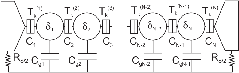
Let us consider a 1d array of quantum dots connected in series chaotic quantum dots (Fig. 3). Each quantum dot is characterized by its own mean level spacing . Adjacent quantum dots are connected to each other via barriers which can scatter electrons. The first and the last dot are also connected to the leads (with total resistance ), i.e. altogether we have scatterers in our system. Each such scatterer is described by a set of transmissions of its conducting channels (here labels the channels and labels the scatterers). Below we will focus our attention on the case of metallic quantum dots with the level spacing being the lowest energy parameter in the problem.
The system of Fig. 3 will be described by the Hamiltonian
| (3) | |||||
where is the capacitance matrix of the array, is the operator of electric potential on th quantum dot,
are the Hamiltonians of the left and right leads, are the electric potentials of the leads fixed by the external voltage source,
is the Hamiltonian of -th quantum dot and is a random matrix which belongs to the orthogonal ensemble. Finally, electron transfer between adjacent -th and -th quantum dots will be described by the Hamiltonian
Here the integration runs over the junction area.
Note that in Ref. [48] we have already applied the model of Fig. 3 in order to analyze WL effects in the absence of electron-electron interactions. In that paper we have used the scattering matrix formalism combined with the non-linear -model. In order to incorporate interaction effects into our consideration it will be convenient for us to describe inter-dot electron transfer within the tunneling Hamiltonian approach, as specified above. We would like to emphasize that this choice is only a matter of technical convenience, since the approaches based on the tunneling Hamiltonian and on the scattering matrix are fully equivalent to each other.
For the sake of completeness, let us briefly remind the reader the relation between these two approaches. Consider, e.g., the -th barrier between the -th and -th quantum dots and define the matrix elements between the th wave function in the -th dot and th wave function in the -th dot. Electron transfer across this barrier can then be described by the set of eigenvalues of this matrix . These eigenvalues are related to the barrier channel transmissions as ( see, e.g., [49])
| (4) |
This equation allows to keep track of the relation between two approaches at every stage of the calculation.
To proceed we will make use of the path integral Keldysh technique. A brief sketch of this approach is outlined below. The time evolution of the density matrix of our system is described by the standard equation
| (5) |
where is given by Eq. (3). Let us express the operators and via path integrals over the fluctuating electric potentials defined respectively on the forward and backward parts of the Keldysh contour:
| (6) |
Here () stands for the time ordered (anti-ordered) exponent and the Hamiltonians , are obtained from the original Hamiltonian (3) if one replaces the operators respectively by the fluctuating voltages and .
The central object of our analysis is the effective action defined as
| (7) | |||||
Since the operators , are quadratic in the electron creation and annihilation operators, it is possible to rewrite the action in the form
| (8) |
where is the inverse Keldysh Green function of the system. The operator has the following matrix structure
Here each quantum dot as well as each of the two leads is represented by a diagonal block
while barriers are described by off-diagonal blocks , which have the form
| (19) |
Below we will employ these general expressions in specific situations of two quantum dots and of an array with a large number of quantum dots. The latter system will also serve as a model for spatially extended diffusive conductors.
4 System of three barriers
Let us first consider the system of three scatterers (two quantum dots). This system is important both in the context of electron dephasing in quantum dots [32, 33, 34, 35, 36] and as a relatively simple example which illustrates all significant features of the effect of electron-electron interactions on WL in more complicated systems.
Here we will treat interaction effects practically without any approximations. For the sake of simplicity we will assume that the central (i.e. second) barrier is a tunnel junction with for all its transmission channels. This assumption allows one to expand the action (8) in powers of the parameter . We will also assume that dimensionless conductance of the central barrier is much lower than those of the first and third barriers which, in turn, strongly exceed unity, i.e, . The effective expansion parameter in this case is . Then the WL correction to the conductance in the absence of interactions takes a particularly simple form [48]. E.g., for fully open outer barriers we have
| (20) | |||||
| (21) |
The first term in Eq. (20) defines the contribution of the first and third scatterers, while the term comes from the central junction. Experimentally one can access attaching additional voltage probes to the quantum dots. The aim of our subsequent analysis is to demonstrate how the result (21) is modified in the presence of electron-electron interactions.
4.1 WL correction in the presence of interactions
Setting in Eq. (3) and defining the fluctuating phases across the barriers we perform the gauge transformation which yields the new expressions for the blocks and :
| (22) |
| (23) |
Since the central barrier transmission is small we can expand the action (8) in powers of the parameter . Proceeding with this expansion up to the fourth order we get
| (24) |
Here
| (25) |
is the effective action at zero transmission of the second barrier which also includes terms describing capacitances () and the external circuit (), the term is the standard Ambegaokar-Eckern-Schön (AES) action [43] and contains information which will allow us to evaluate the WL correction to the system conductance. The corresponding expression reads
| (26) | |||||
Here we use the convention , , , and are matrix Green-Keldysh functions in the first and the second quantum dots ():
Here we will set the Green functions and equal to their equilibrium values , where are retarded and advanced Green functions,
| (30) |
is the Fermi function and . This choice is sufficiently accurate for the problem in question. We will return to this point towards the end of this section.
Our next step amounts to averaging the products of retarded and advanced propagators in the action (26) over disorder in each of the two dots separately. This averaging can be accomplished, e.g., with the aid of the non-linear -model or by other means. For the first (left) dot we obtain (cf., e.g., [54])
| (31) |
where is the volume of the first (left) quantum dot, , and are respectively the density of states, the diffuson and the Cooperon in the first (left) dot, , and are respectively the Fermi wave vector and elastic mean free path. The same averaging procedure applies to the second (right) dot. In the absence of magnetic field both the diffuson and the Cooperon satisfy the same diffusion equation
| (32) |
with the appropriate boundary conditions at the contacts.
Averaging the action (26) over disorder we will collect only the terms proportional to the product of the Cooperons and and ignore all other contributions which are unimportant for the problem in question. In this way we arrive at the action which describes weak localization effects in our system. Ignoring for simplicity the coordinate dependence of the Cooperons inside the dots, we obtain
| (33) |
Here we defined mean level spacing for both dots, introduced “classical” and “quantum” phases and made use of the Fourier transforms of the Fermi function . The resulting action (33) fully accounts for the effects of electron-electron interactions on WL via the fluctuating phases .
In order to find the WL correction to the current across the central barrier we employ the following general formula
| (34) |
The task at hand is to combine Eqs. (33) and (34) and to average over the phases by evaluating the path integral in (34). The contributions and in (25) are quadratic in the fluctuating phases provided an external circuit consists of linear elements. The remaining contribution to (25) which describes transfer of electrons across the first and third barriers as well as AES action of the second barrier are in general non-Gaussian. However, in the interesting limit phase fluctuations can be considered small down to exponentially low energies [55, 56] in which case it suffices to expand both contributions and up to the second order . Furthermore, Gaussian approximation for the first of these terms becomes essentially exact in the limit of fully open outer barriers with [57].
We conclude that the integral (34) remains Gaussian at all relevant energies and can easily be performed. After straightforward algebra we arrive at the final result
| (35) |
Here is the average voltage across the central barrier, are the Fourier transforms of the Cooperons and the functions () are defined as
| (36) |
where
| (37) |
| (38) |
and coincides with the phase correlation function (2). The terms read
| (39) |
where is the response function. Eqs. (35)-(39) fully determine WL correction to the current in our system. The non-interacting result [48] is reproduced by the first line of Eq. (35), while its second and third lines exactly account for the effect of interactions. We observe that the whole effect of electron-electron interactions is encoded in two different correlators of fluctuating phases and defined as
| (40) | |||||
| (41) |
where is an effective impedance “seen” by the central barrier.
Let us recall that these correlation functions play a central in the so-called -theory of Coulomb blockade in tunnel barriers [43, 58]. It turns out that exactly the same correlators also describe the effect of electron-electron interactions on weak localization. Below we will demonstrate that the phase correlation function (40) is responsible for electron dephasing while the response function (41) describes the Coulomb blockade correction to WL.
4.2 Dephasing
Let us now turn to the analysis of the above general results. To begin with, we notice that both functions (40) and (41) are purely real and, hence, . Furthermore, at sufficiently long times (where is an effective -time of our system to be defined later) we obtain
| (42) | |||||
| (43) |
where , and is the Euler constant. The correlation function grows with time [59] at any temperature including . In contrast, the response function always remains small in the limit considered here. Hence, the combination (38) should be fully kept in the exponent of (37) while the correlator can be safely ignored in the leading order in . Then all , the Fermi function drops out from the result and we get , where
| (44) | |||||
where
| (45) |
Identifying and in Eq. (45) we observe that the exponent exactly coincides with the expression (1) derived from simple considerations involving electrons propagating along time-reversed paths in an external fluctuating field. Thus, we arrive at an important conclusion: In the leading order in the WL correction is affected by electron-electron interactions via dephasing produced only by the “classical” component of the fluctuating field which mediates such interactions. This effect is described only by the phase correlation function (40). At the same time, fluctuations of the “quantum” field turn out to be irrelevant for dephasing and may only cause a (weak) Coulomb blockade correction described by the response function (41). This latter effect will be analyzed in the next subsection.
In order to simplify our consideration let us assume that two quantum dots are identical, i.e. and , and set . In this case the Cooperons are , where is the dwell time for each of the two dots and is the dephasing time due to the external magnetic field which can be applied to the system. An effective impedance takes the form
| (46) |
where , , and , and are the capacitances of respectively left(right) barriers, the central junction and the gate electrode. Substituting the Cooperons into Eq. (47) we arrive at the final expression for the WL correction in the presence of electron-electron interactions
| (47) |
With a good accuracy the double time integral in Eq. (47) can be replaced by a single one, in which case the magnetoconductance can be expressed in a much simpler form
| (48) |
The result (47) for is plotted in Fig. 4. We observe that electron-electron interactions always suppress below its non-interacting value (21). This is a direct consequence of interaction-induced electron dephasing described by the correlation function .

Let us define and consider the limit of metallic dots . At and for we find
| (49) |
whereas at the WL correction saturates to
| (50) |
Let us compare the magnitude of the WL correction (50) to that of the leading contribution to the system conductance evaluated in the presence of electron-electron interactions. This contribution reads [60, 43, 58]
| (51) |
where is the gamma-function. Setting in the above expression, we observe that the WL correction (50) remains much smaller than Eq. (51) by the parameter .

Let us phenomenologically define the electron decoherence time by taking the Cooperons (for ) in the form . This definition obviously yields [48] . Resolving this equation with respect to , we obtain
| (52) |
Substituting the result (49) into Eq. (52) at sufficiently high temperatures and in the limit we obtain
| (53) |
Combining Eqs. (50) and (52) at lower temperatures and for we find
| (54) |
In the limit of large this expression yields
| (55) |
The results for the electron decoherence time (52) are also plotted in Fig. 5 for different values of . We observe that at higher temperatures shows a -dependent power law dependence on and eventually saturates to the value (55) at lower . This is exactly the behavior observed in a number of experiments with quantum dots [32, 33, 34, 35, 36]. We will postpone a detailed comparison between our theory and experiments to Sec. 6.
4.3 Perturbation theory and Coulomb correction to weak localization
Let us now analyze the role of the response function which was disregarded in the previous subsection. For this purpose let us expand the general expression for the current (35) to the first order in the interaction, i.e. to the first order in both and . We get
| (56) |
where
| (57) |
| (58) |
Here we defined the function
The above expressions allow to make several important observations. To begin with, we note that the term is linear in the bias voltage while is non-linear in . The physical meaning of these two terms is entirely different. While, as we already know, the correction describes electron dephasing, the term is nothing but the Coulomb blockade correction to (47). The latter conclusion is supported, for instance, by the observation that at large voltages tends to a constant offset value, which is a typical sign of Coulomb blockade.
Just for the sake of illustration, let us for a moment assume that the environment remains Gaussian at all energies. In this case diverges at indicating the importance of higher order perturbative terms in the low energy limit. Making use of analytical properties of the functions one can exactly sum up diverging perturbative series to all orders and quite generally demonstrate that in the limit of zero voltage and temperature the WL correction tends to zero, , implying complete Coulomb suppression of weak localization in this limit. This strong Coulomb blockade of WL can be recovered only if one fully accounts for the response function . We also note that at large conductances weak Coulomb blockade may turn into strong one only at exponentially small energies [55, 56] typically well below the inverse electron dwell time , otherwise Coulomb suppression of WL remains weak.
Turning back to the first order terms (57) and (58), we observe that in the linear response regime almost all contributions from and cancel each other exactly in the limit . This (partial) cancellation of the so-called “coth”(57) and “tanh” (58) terms is a general feature of the first order perturbation theory. For instance, in diffusive conductors it has been observed by various authors [61, 62]. This cancellation is sometimes interpreted as a “proof” of zero dephasing of interacting electrons at assuming that the same “coth-tanh” combination should occur in every order of the perturbation theory [63]. Our exact result (35) demonstrates, that this assumption is incorrect. Partial cancellation between dephasing and Coulomb blockade terms occurs only in the first order and is of little importance for the issue of electron dephasing. Actually, the combination enters only in the first order, while the exact expression (35) depends on and and does not contain the combination at all. This observation is fully consistent with our general result for the WL correction [40] expressed in terms of the matrix elements of the operators and , where is the electron density matrix. In fact, the analysis presented above is a way to explicitly evaluate these matrix elements for a particular case of two quantum dots.
Finally, let us estimate the corrections and . For max we obtain
| (59) | |||
i.e. at the ratio of the terms (4.3) and (59) is of order and it decreases further with increasing temperature as . This estimate demonstrates that can be ignored as compared to the main contribution . This conclusion remains valid also beyond the first order perturbation theory. Indeed, keeping the function in the exponent of Eq. (35) and expanding this result only in powers of , at one finds
| (63) |
thus supporting our conclusion about relative unimportance of the Coulomb blockade correction to for the problem in question.
4.4 Summary of approximations
For clarity, let us again summarize all the approximations used in the above analysis:
Throughout our calculation we have used the equilibrium form of the distribution function matrices (30) which effectively implies neglecting the dependence of the Green functions on the phases and . This is accurate except at energies well below the inverse dwell time . The WL correction (44)-(45) saturates at energies and, hence, is totally insensitive to this approximation. The Coulomb term should be treated somewhat more carefully in the limit . For this treatment also yields saturation of the Coulomb correction to WL at energies of order , exactly as in the case of the interaction correction to the Drude conductance [50, 64]. In other words, at all the term remains constant of order . Thus, the above approximation is completely unimportant for any of our conclusions.
We have assumed and . The first inequality just implies that our structure is metallic, while the second one is only a matter of technical convenience. Obviously, our results for remain qualitatively the same also for .
For completeness, let us also mention that in the final expressions for , e.g., in Eqs. (49) and (50), we have disregarded small renormalization of the conductance due to Coulomb effects [52, 53]. This renormalization is strictly zero for fully open outer barriers, otherwise it can be trivially included into our final results.
5 Arrays of quantum dots and diffusive conductors
One of the main conclusions reached in the previous section is that the electron decoherence time is fully determined by fluctuations of the phase fields (and the correlation function ), whereas the phases (and the response function ) are irrelevant for causing only a weak Coulomb correction to . This conclusion is general being independent of a number of scatterers in our system. Note that exactly the same conclusion was already reached in the case of diffusive metals by means of a different approach [38, 39, 40]. Thus, in order to evaluate the decoherence time for interacting electrons in arrays of quantum dots it is sufficient to account for the fluctuating fields totally ignoring the fields . The corresponding calculation is presented below. We will specifically address the example of 1d arrays and argue that the final result for the zero temperature decoherence time actually does not depend on the dimensionality of the array. We will also demonstrate how our present results for match with those obtained previously for weakly disordered metals [37, 38, 39].
5.1 1d structures
Let us consider a 1D array of quantum dots by identical barriers as shown in Fig. 3. For simplicity, we will stick to the case of identical barriers (with dimensionless conductance and Fano factor ) and identical quantum dots (with mean level spacing and dwell time ). The WL correction to the system conductance has the form [48]
| (64) | |||||
The Cooperon is determined from a discrete version of the diffusion equation. For non-interacting electrons and in the absence of the magnetic field this equation reads
| (65) |
The boundary conditions for this equation are as long as the index or belongs to one of the bulk electrode. The solution of Eq. (65) with these boundary conditions can easily be obtained. We have
| (66) |
This solution can be represented in the form , where
| (67) |
In the limit of large the term can be safely ignored and we obtain . Let us express the contribution as a sum over the integer valued paths , which start in the th dot and end in the th one (i.e. , ) jumping from one dot to another at times . This expression can be recovered if one expands Eq. (67) in powers of with subsequent summation over in every order of this expansion. Including additional phase factors acquired by electrons in the presence of the fluctuating fields , we obtain
| (68) |
Averaging over Gaussian fluctuations of voltages and utilizing the symmetry of the voltage correlator , we get
| (69) |
The correlator of voltages can be obtained, e.g., with the aid of the -model approach employed in Ref. [48]. Integrating over Gaussian fluctuations of the -fields one arrives at the quadratic action for the fluctuating fields which has the form
| (70) |
Here we defined
| (71) |
The action (70) determines the expressions for both correlators (-function) and (-function) responsible respectively for decoherence and Coulomb blockade correction to WL. Since our aim is to describe electron decoherence, only the first out of these two correlation functions is of importance for us here. It reads
| (72) |
In the continuous limit and for sufficiently low frequencies both correlators and defined by Eq. (70) reduce to those of a diffusive metal [38].
To proceed let us consider diffusive paths , in which case one has
| (73) | |||||
where is the diffuson. For it exactly coincides with the Cooperon for non-interacting electrons (66), , i.e.
| (74) |
Substituting Eq. (73) into (69), we obtain
| (75) |
where
| (76) | |||||
is the function which controls the Cooperon decay in time, i.e. describes electron decoherence for our 1d array of quantum dots. The WL correction in the presence of electron-electron interactions is recovered by substituting the result (75) into Eq. (64).
Note that in the limit of very large and for Eq. (76) (combined with (72) and (74)) reduces to Eq. (22) of Ref. [39] derived for metallic conductors by means of a different technique. Replacing the sum in (76) by momentum integration, in the same limit one arrives at the result which matches with Eq. (23) of [39] provided one sets the charging energy terms equal to zero.
Since the behavior of the latter formula was already analyzed in details earlier [39], there is no need to repeat this analysis here. The dephasing time can be extracted from the equation . From Eq. (76) with a good accuracy we obtain
| (77) |
Combining this formula with Eqs. (72) and (74), in the most interesting limit and for we find
which yields
| (78) |
where for and in the opposite case .
We observe that apart from an unimportant numerical factor of order one the result for (78) derived for 1d array of quantum dots coincides with the exact result (55) derived in the previous section for the case of two quantum dots. Thus, we arrive at an important conclusion: In the low temperature limit the electron decoherence time is practically independent of the number of scatterers in the conductor (provided the latter number exceeds two) and is essentially determined by local properties of the system.
In order to determine the dephasing length let us define the diffusion coefficient
| (79) |
where is the average dot size. Combining Eqs. (78) and (79), at we obtain
| (80) |
At non-zero thermal fluctuations provide an additional contribution to the dephasing rate . Again substituting Eqs. (72) and (74) into (77), we get
| (81) |
where is the number of quantum dots within the length . We observe that for sufficiently small (but still ) the dephasing rate increases linearly both with temperature and with the number . At larger and/or at high enough temperatures becomes smaller than and Eq. (81) for should be resolved self-consistently. In this case we obtain
| (82) |
which matches with the AAK result [65]. Eq. (81) also allows to estimate the temperature at which the crossover to the temperature-independent regime (78) occurs. We find
| (83) |
5.2 Good metals and granular conductors
The above analysis and conclusions can be generalized further to the case 2d and 3d structures. This generalization is absolutely straightforward (see, e.g. [48]) and therefore is not presented here. At one again arrives at the same result for (78).
Now we discuss the relation between our present results and those derived earlier for weakly disordered metals by means of a different approach [37, 38, 39]. Let us express the dot mean level spacing via the average dot size as (where is the electron density of states at the Fermi level). Then we obtain
| (84) |
Below we consider two different physical limits of good metals and strongly disordered (granular) conductors. For the model we assume that quantum dots are in a good contact with each other. In this case scales linearly with the contact area , where is a numerical factor of order (typically smaller than) one which particular value depends on geometry. For weakly disordered metals most conducting channels in such contacts can be considered open. Hence, and
| (85) |
i.e. . Comparing this estimate with the standard definition of for a bulk diffusive conductor, , we immediately observe that within our model the average dot size is comparable to the elastic mean free path, , as it should be for weakly disordered metals.
Expressing (78) via , in this limit we get
| (86) |
where is the electron mass and is constant which depends on . Estimating, e.g., , one obtains .
Note that apart from an unimportant numerical pre-factor and the logarithm in the denominator of Eq. (86) the latter result for coincides with that derived in Refs. [37, 38, 39] for a bulk diffusive metal within the framework of a completely different approach, cf., e.g., Eq. (81) in [38]. Within that approach local properties of the model could not be fully defined. For this reason in the corresponding integrals in [37, 38, 39] we could not avoid using an effective high frequency cutoff procedure which yields the correct leading dependence and it only does not allow to recover an additional logarithmic dependence on in (86). Our present approach is divergence-free and, hence, it does not require any cutoffs.
We can also add that Eq. (78) also agrees with our earlier results [37, 38, 39] derived for quasi-1d and quasi-2d metallic conductors. Provided the transversal size of our array is smaller than one should set for 2d and for 1d conductors. Then Eq. (78) yields and respectively in 2d and 1d cases. Up to the factor these dependencies coincide with ones derived previously, cf., e.g., Eq. (32) in [39].
Now let us turn to the model of strongly disordered or granular conductors. In contrast to the situation , we will assume that the contact between dots (grains) is rather poor, and inter-grain electron transport may occur only via a limited number of conducting channels. In this case the average dimensionless conductance can be approximated by some -independent constant . Substituting instead of into Eq. (84) we observe that in the case of strongly disordered structures one can expect . Accordingly, for (78) one finds
| (87) |
where again depends on . For we have . Hence, the dependence of on for strongly disordered or granular conductors (87) is it qualitatively different from that for sufficiently clean metals (86).
One can also roughly estimate the crossover between the regimes and by requiring the values of (85) and to be of the same order. This condition yields , and we arrive at the estimate for at the crossover
| (88) |
Here we restored the Planck constant set equal to unity elsewhere in our paper.
In the next section we will use the above results and carry out a detailed comparison between our theory and numerous available experimental data for in different types of disordered conductors.
6 Comparison with experiments
Turning to experiments, it is important to emphasize again that low temperature saturation of the electron decoherence time has been repeatedly observed in numerous experiments and is presently considered as firmly established and indisputably existing phenomenon. At the same time, the physical origin of this phenomenon still remains under debate. The key observations and remaining controversies are briefly summarized below.
- 1.
The authors [36] have analyzed the values of observed in their experiments with open quantum dots as well in earlier experiments by different groups [32, 33, 34, 35]. For all 14 samples reported in [32, 33, 34, 35, 36] the values were found to rather closely follow a simple dependence
(89) This approximate scaling was observed within the interval of dwell times of about 3 decades, see Fig. 5 in Ref. [36]. To the best of our knowledge, until now no physical interpretation of this observation has been suggested.
- 2.
In some of our earlier publications [37, 38, 45, 46] we have demonstrated a good quantitative agreement between our theoretical predictions [37, 38] and experimental data for obtained for numerous metallic wires and quasi-1d semiconductors. As our theory of dephasing by electron-electron interactions [37, 38] predicts a rather steep increase of with the system diffusion coefficient , e.g. for most metals as , we can conclude that for a large number of disordered conductors strongly increases with increasing .
- 3.
In a series of papers, see, e.g., Refs. [26, 27, 31, 47], Lin and coworkers analyzed numerous experimental data for obtained by various groups in disordered conductors with cm2/s and observed systematic decrease of with increasing . The data could be rather well fitted by the dependence with the power . This trend is opposite to one observed in less disordered conductors with cm2/s and remained unexplained until now.
- 4.
The authors [62] pointed out a disagreement between our expressions for [37, 38] and the data obtained for a number of typically rather strongly disordered 2d and 3d structures. In some cases this disagreement was argued to be as large as 4 to 5 orders of magnitude. In Ref. [66] we countered this critique showing, on one hand, reasonable agreement for some of the samples in question and arguing, on the other hand, that our quasiclassical theory [37, 38] is applicable merely to weakly disordered conductors. Hence, it cannot be used in order to quantitatively describe strongly disordered structures like, e.g., granular metals, metallic glasses etc. quoted in Ref. [62]. Formally eliminating the controversy, this our argument, however, did not yet allow to clarify the issue of low temperature saturation of in strongly disordered conductors which remained unclear until now.
- 5.
Pierre et al. [7] argued that low temperature saturation of in sufficiently clean samples can be caused by undetectably small number of magnetic impurities. This idea, however, was not supported by the authors [8] who demonstrated that at least in their experiments (performed in high magnetic fields in order to fully polarize any magnetic moments should they exist) the observed -saturation cannot be due to magnetic impurities. Later the issue was reanalyzed in Refs. [12, 14, 15, 16] on the basis of recently developed numerical renormalization group (NRG) theory of electron scattering by Kondo impurities [67]. In samples with implanted magnetic impurities a very good agreement between theory [67] and experiments [14, 15, 16] was demonstrated both above and below the Kondo temperature . However, at significant deviations from NRG predictions was observed and was found to saturate [14, 15, 16] in all samples both with and without magnetic impurities. Interpretation of this saturation effect in terms of both underscreened and overscreened models is problematic [14, 16].
Let us now analyze the above problems and controversies point by point within the framework of our theory of electron-electron interactions.
We start from the case of quantum dots [32, 33, 34, 35, 36] observe that our results for (55), (78) scale practically linearly with the dwell time which is essentially the scaling (89) suggested in Ref. [36]. There is, however, one point which requires a comment.
As it was argued in Sec. 2, one should expect no dephasing by electron-electron interactions in single quantum dots at any . Naively one could regard this statement as yet one more controversy with experiments [32, 33, 34, 35, 36] where electron dephasing in single dots was clearly observed. At this stage let us recall that qualitative arguments in Sec. 2 as well as rigorous analysis in Refs. [50, 51] remain applicable to single dots provided fluctuating voltages drop strictly across the two barriers. In realistic quantum dots [32, 33, 34, 35, 36] fluctuating voltages most likely penetrate inside rather than drop only at the edges. Within the framework of our model one can easily mimic this situation by introducing additional scatterers inside the dot in which case fluctuating voltages already do dephase (see Sec. 2).
For illustration, let us consider a strongly asymmetric double dot system, i.e. we replace, say, the left barrier in Fig. 1 by a small quantum dot with the electron flight time . The left dot will then model a barrier of a finite length in a single dot configuration of Fig. 1. Applying Eqs. (44), (57) and (58), we evaluate the WL correction and again arrive at Eqs. (49-50), where, however, . Extracting the decoherence time , we obtain
| (90) |
for and vanishing decoherence rate in the opposite limit . Provided the denominator in Eq. (90) is not very large, we arrive at Eq. (89). We also note that in a single dot (90) is always longer than that in a system of two dots (54).
Alternatively, one can model a dot by a chain of several () scatterers with defined in Eqs. (78), (81), (82). Then at higher temperatures we obtain with ranging from 2/3 to 1, as observed in a number of dots [32, 33, 34, 35, 36]. Substituting by (where are are respectively the dimensionless conductance and the dwell time of a composite dot), bearing in mind that [36] and assuming to be not very large, at low from (78) one finds in agreement with experimental results presented in Fig. 5 of Ref. [36]. More complicated configurations of scatterers can also be considered with essentially the same results. We conclude that our present theory is in a good agreement with experimental findings [32, 33, 34, 35, 36].
Let us now turn to experiments with spatially extended conductors. In Fig. 6 we have collected experimental data for obtained in over 120 metallic samples with diffusion coefficients varying by decades, from cm2/s to cm2/s. The data were taken from about 30 different publications listed in figure caption. We see that the the measured values of strongly depend on . Furthermore, this dependence turns out to be non-monotonous: For relatively weakly disordered structures with cm2/s clearly increases with increasing , while for strongly disordered conductors with cm2/s the opposite trend takes place. In addition to the data points in Fig. 6 we indicate the dependencies (86) and (87) for two models and discussed in Sec. 5.2.

We observe that for cm2/s the data points clearly follow the scaling (86). Practically all data points remain within the strip between the two lines corresponding to Eq. (86) with (dashed line) and (solid line). On the other hand, for more disordered conductors with cm2/s the data are consistent with the scaling (87) obtained within the model . We would like to emphasize that theoretical curves (86) and (87) are presented in Fig. 6 without any additional fit parameters except for a geometry factor for the first dependence and the value for the second one. This value of was estimated from the crossover condition (88) with cm2/s and .
Note that quite a few data points with cm2/sek correspond to the samples contaminated by magnetic impurities. Remarkably, these data points also demonstrate – though with somewhat larger scatter – systematic increase of with increasing . At the same time, for similar values of the samples with higher concentration of magnetic impurities have systematically lower than samples with few or no magnetic impurities. These observations indicate that for samples with relatively high concentration of magnetic impurities both mechanisms of electron-electron interactions and spin-flip scattering provide substantial contributions to , being responsible respectively for the scaling and for additional non-universal shift of the data points downwards.
In order to carry out more accurate comparison with our theory of electron-electron interactions let us now leave out the data points taken from the samples with high concentration of magnetic impurities. In Fig. 7 we selected the data for 37 different metallic wires with no or few magnetic impurities and with diffusion coefficients in the range 9 cm2/s cm2/s from Refs. [4, 5, 6, 7, 8, 9, 10, 11, 12, 14, 15, 16, 69, 70]. Two minor adjustments of some data points are in order. Firstly, in order to eliminate the uncertainty related to different definitions of used by different groups [71], we have adjusted 6 data points [6] and 2 data points [10] according to the definition of used in other works [4, 5, 7, 11, 12, 14, 15]. Secondly, 5 data points corresponding to samples with high diffusion coefficients [7] have been adjusted in order to eliminate the temperature dependent contribution to which remains substantial for these samples down to the lowest mK [72]. Both these adjustments can in no way influence our conclusions (in fact, non-adjusted data points also remain in-between solid and dashed lines in Fig. 7).

The data in Fig. 7 again clearly support the scaling of with (86) due to electron-electron interactions. Practically all data points are now located in-between the solid and dashed lines which indicate the dependence (86) with respectively and . We cannot exclude that the remaining scatter among the data points with similar values of – to a certain extent – may be due to relatively small amount of magnetic impurities possibly residing in some samples. Also minor differences in metal parameters (e.g, Fermi velocities) may contribute to this effect. It appears, however, that sample-to-sample fluctuations of the geometry parameter play the most important role. This parameter is defined as a ratio between the square root of the inter-dot (inter-grain) contact area and the average dot (grain) size , i.e. accounts for local properties of the sample which can be highly non-universal. Electrons in metallic wires get scattered both in the bulk and on the surface. Hence, e.g., the surface quality and/or details of the wire geometry – along with other factors – may significantly impact the value of . Since (86) depends quite strongly on , it is by no means surprising that different wires with similar values of may have decoherence times differing by few times.
As an illustration of this point let us consider 4 quasi-1d AuPd samples C, D, E, F [6] with nominally identical values of cm2/s. Although these samples were fabricated in the same way and measured in one experiment [6], their dephasing times were found to differ by up to times. This difference can hardly be ascribed to magnetic impurities since the measured level of dephasing would require unrealistically high concentration of such impurities (in the range of 100 ppm) and, in addition, rather exotic values of the Kondo temperature . At the same time, sample-to-sample fluctuations of the parameter of only per cent (which is easy to assume given, e.g., somewhat different geometry of the samples) would fully account for the above difference of dephasing times. We conclude that our theoretical expression (86) is in a good quantitative agreement with the available experimental data for quasi-1d metallic wires with diffusion coefficients in the range 9 cm2/s cm2/s.
Now let us return to Fig. 6 and consider the data for strongly disordered conductors with cm2/s. As we already pointed out, the agreement between the data and the dependence (87) predicted within our simple model is reasonable, in particular for samples with cm2/s. At higher diffusion coefficients most of the data points indicate a weaker dependence of on which appears natural in the vicinity of the crossover to the dependence (86). The best fit for the whole range 0.3 cm2/s cm2/s is achieved with the function with the power . Further modifications of our – clearly oversimplified – model can help to achieve even better agreement between theory and experiment.
Although such modifications can certainly be worked out, it is not our aim to do it here. More importantly, our analysis of Sec. 5.2 allows to qualitatively understand and explain seemingly contradicting dependencies of on observed in weakly and strongly disordered conductors. While the trend “less disorder – less decoherence” (86) for sufficiently clean conductors is quite obvious, the opposite trend “more disorder – less decoherence” in strongly disordered structures requires a comment. Effectively the latter dependence implies that with increasing disorder electrons spend more time in the areas with fluctuating in time but spatially uniform potentials which do not dephase, as we also discussed in Sec. 2. In other words, in this case an effective dwell time in Eq. (78) becomes longer with increasing disorder and, hence, the electron decoherence time does so too.
Is the physical picture of decreasing with increasing dot (or grain) size (employed within the model ) realistic? Although for cleaner conductors the tendency is usually just the opposite, for strongly disordered structures increasing resistivity with increasing grain size has been observed in a various experiments [73, 74, 75]. In addition, since local conductance fluctuations increase with increasing disorder, several grains can form a cluster with internal inter-grain conductances strongly exceeding those at its edges. In this case fluctuating potentials remain almost uniform inside the whole cluster which will then play a role of an effective (bigger) grain/dot. Accordingly, the average volume of such “composite dots” may grow with increasing disorder, electrons will spend more time in such bigger dots and, hence, the electron decoherence time (78) will increase.
The above comparison with experiments confirms that our previous quasiclassical results for [37, 38, 39] are applicable to relatively weakly disordered structures with cm2/s, while for conductors with stronger disorder different expressions for (e.g., Eq. (87)) should be used. For instance, the claimed in Ref. [62] “disagreement” between our theory and some experiments by 4 to 5 orders of magnitude is solely due to misuse of our results [37, 38] far beyond their applicability range. A glance at Fig. 6 is sufficient to realize that any attempt to apply Eq. (86) to structures with, e.g., cm2/s can easily lead to a “disagreement” with the data, say, by 6 orders of magnitude or so. This observation, however, does not imply any real disagreement, rather it indicates that more general results for , e.g., Eq. (78), should be used. The same argument invalidates the comparison between our quasiclassical results [37, 38] and the data for the sample Au-5 [4], see Fig. 8 of Ref. [7], or, to a somewhat lesser extent, for the sample C of Ref. [11], see Table II of that paper [76].
Finally, our analysis allows to rule out scattering on magnetic impurities as a cause of low temperature saturation of . This mechanism can explain neither strong and non-trivial dependence of the electron decoherence time on (see our Figs. 6 and 7 as well as, e.g., Fig. 4 in [18], Fig. 1 in [27] and Fig. 5 in [36]) nor even the level of dephasing observed in numerous experiments. E.g., in order to be able to attribute dephasing times as short as s to magnetic impurities one needs to assume huge concentration of such impurities ranging from few hundreds to few thousands ppm which appears highly unrealistic, in particular for systems like carbon nanotubes, 2DEGs or quantum dots. Similar arguments were independently emphasized by Lin and coworkers [27, 47]. Even in metallic wires with high values of and long dephasing times, at one observes clear saturation of [12, 14, 15] which is in a quantitative agreement with our theory of electron-electron interactions (see Fig. 7) and is very hard to explain otherwise [16].
Thus, although electron dephasing due to scattering on magnetic impurities is by itself an interesting issue, its role in low temperature saturation of in disordered conductors is sometimes strongly overemphasized. Since the latter phenomenon has been repeatedly observed in all types of disordered conductors, the physics behind it should most likely be universal and fundamental. We believe – and have demonstrated here – that it is indeed the case: Zero temperature electron decoherence in all types of conductors discussed above is caused by electron-electron interactions.
7 Conclusions
In this paper we have employed a model of an array of quantum dots/scatterers (Fig. 3) which embraces various types of disordered conductors and allows to study electron transport in the presence of interactions within a very general theoretical framework. We have non-perturbatively analyzed the impact of electron-electron interactions on weak localization for such structures with the emphasis put on the interaction-induced decoherence of electrons at low temperatures. We have formulated a fully self-contained theory free of any divergencies and cutoffs which allows to conveniently handle disorder averaging and treat electron scattering without residing to quasiclassics. In the case of two quantum dots (or three scatterers) it was possible to find an exact solution of the problem (Sec. 4) and to evaluate the WL correction to the system conductance practically without approximations.
With the aid of our approach we have formulated a unified description of electron dephasing by Coulomb interaction in different structures including (i) weakly disordered conductors (e.g., metallic wires with cm2/s), (ii) strongly disordered conductors ( cm2/s) and (iii) metallic quantum dots. We have demonstrated that in all these cases at the electron decoherence time is determined by the same simple formula . In the case (i) this formula yields and matches with our previous quasiclassical results [37, 38, 39] while in the cases (ii) and (iii) it illustrates new physics which was not yet explored before. In particular, this formula emphasizes the dependence of on the electron dwell time in single quantum dots [36] and helps to understand the (at the first sight counterintuitive) trend “more disorder – less decoherence” observed in strongly disordered conductors [26, 27, 31, 47].
We have carried out a detailed comparison of our theoretical predictions with the results of numerous experiments for the whole scope of structures (i), (ii) and (iii) (Sec. 6). In all cases we found a good agreement between theory and experiment which further supports our main conclusion that low temperature saturation of is universally caused by electron-electron interactions.
Acknowledgments
We are grateful to C. Bauerle, J. Bird, P. Hakonen, P. Mohanty, D. Natelson, M. Paalanen, J.-J. Lin, L. Saminadayar and R.A. Webb for useful discussions on various experimental aspects of electron decoherence and/or for providing us with their experimental data.
This work is part of the European Community’s Framework Programme NMP4-CT-2003-505457 ULTRA-1D ”Experimental and theoretical investigation of electron transport in ultra-narrow one-dimensional nanostructures”.
References
- [1] G. Bergmann, Phys. Rep. 107 (1984) 1.
- [2] B.L. Altshuler, A.G. Aronov, in Electron-electron interactions in disordered conductors, eds. A.L. Efros and M. Polak, Elsevier Science publishers B.V., New York (1985).
- [3] S. Chakravarty, A. Schmid, Phys. Rep. 140 (1986) 193.
- [4] P. Mohanty, E.M.Q. Jariwala, R.A. Webb, Phys. Rev. Lett. 78 (1997) 3366.
- [5] R.A. Webb, P. Mohanty, E.M.Q. Jariwala, Fortsch. Phys. 46 (1998) 779.
- [6] D. Natelson, R.L. Willett, K.W. West, L.N. Pfeiffer, Phys. Rev. Lett. 86 (2001) 1821.
- [7] F. Pierre, A.B. Gougam, A. Anthore, H. Pothier, D. Esteve, N.O. Birge, Phys. Rev. B 68 (2003) 085413.
- [8] P. Mohanty, R.A. Webb, Phys. Rev. Lett. 91 (2003) 066604.
- [9] F. Schopfer, C. Bäuerle, W. Rabaud, L. Saminadayar, Phys. Rev. Lett. 90 (2003) 056801.
- [10] J.F. Lin, J.P. Bird, L. Rotkina, P.A. Bennett, Appl. Phys. Lett. 82 (2003) 802; J.F. Lin, J.P. Bird, L. Rotkina, Physica E 19 (2003) 112.
- [11] A. Trionfi, S. Lee, D. Natelson, Phys. Rev. B 72 (2005) 035407.
- [12] C. Bäuerle, F. Mallet, F. Shopfer, D. Mailly, G. Eska, L. Saminadayar, Phys. Rev. Lett. 95 (2005) 266805.
- [13] P. Wakaya, Y. Tsukatani, N. Namasaki, K. Murakami, S. Abo, M. Takai, J. Phys.: Conf. Series 38 (2006) 120.
- [14] F. Mallet, J. Ericsson, D. Mailly, S. Unlubayir, D. Reuter, A. Melnikov, A.D. Wieck, T. Micklitz, A. Rosch, T.A. Costi, L. Saminadayar, C. Bäuerle, Phys. Rev. Lett. 97 (2006) 226804.
- [15] G.M. Alzoubi, N.O. Birge, Phys. Rev. Lett. 97 (2006) 226803.
- [16] L. Saminadayar, P. Mohanty, R.A. Webb, P. Degiovanni, C. Bäuerle, Physica E (2007), this volume.
- [17] D.M. Pooke, N. Paquin, M. Pepper, A. Gundlach, J. Phys.: Condens. Matter 1 (1989) 3289.
- [18] M. Noguchi, T. Ikoma, T. Odagiri, H. Sakakibara, S.N. Wang, J. Appl. Phys. 80 (1996) 5138.
- [19] Yu.B. Khavin, M.E. Gershenson, A.L. Bogdanov, Phys. Rev. Lett. 81 (1998) 1066.
- [20] L. Langer, V. Bayot, E. Grivei, J.-P. Issi, J. P. Heremans, C.H. Olk, L. Stockman, C. Van Haesendonck, Y. Bruynseraede, Phys. Rev. Lett. 76 (1996) 479.
- [21] N. Kang, J.S. Hu, W.J. Kong, L. Lu, D.L. Zhang, Z.W. Pan, S.S. Xie, Phys. Rev. B 66 (2002) 241403.
- [22] R. Tarkiainen, M. Ahlskog, A. Zyuzin, P. Hakonen, M. Paalanen, Phys. Rev. B 69 (2004) 033402.
- [23] J.J. Lin, N. Giordano, Phys. Rev. B 35 (1987) 585.
- [24] A. Sahnoune, J.O. Strom-Olsen, H.E. Fisher, Phys. Rev. B 46 (1992) 10035.
- [25] P.M. Echternach, M.E. Gershenson, H.M. Bozler, Phys Rev. B 47 (1993) 13659.
- [26] J.J. Lin, J.P. Bird, J. Phys.: Condens. Matter 14 (2002) R501, and further references therein.
- [27] J.J. Lin, T.C. Lee, S.W. Wang, Physica E (2007) this volume, see also further references therein.
- [28] G. Brunthaler, A. Prinz, G. Bauer, V.M. Pudalov, Phys. Rev. Lett. 87 (2001) 096802.
- [29] Y.Y. Proskuryakov, A.K. Savchenko, S.S. Safonov, M. Pepper, M.Y. Simmons, D.A. Ritchie, Phys. Rev. Lett. 86 (2001) 4895.
- [30] Y. Yaish, O. Prus, E. Buchstab, G. Ben Yosef, U. Sivan, I. Ussishkin, A. Stern, cond-mat/0109469.
- [31] J.J. Lin, L.Y. Kao, J. Phys.: Condens. Matter 13 (2001) L119.
- [32] J.P. Bird, K. Ishibashi, D.K. Ferry, Y. Ochiai, Y. Aoyagi, T. Sugano, Phys. Rev. B 51 (1995) 18037.
- [33] R.M. Clarke, I.H. Chan, C.M. Marcus, C.I. Duruoz, J.S. Harris, K. Campman, A.C. Gossard, Phys. Rev. B 52 (1995) 2656.
- [34] D.P. Pivin, A. Andresen, J.P. Bird, D.K. Ferry, Phys. Rev. Lett. 82 (1999) 4687.
- [35] A.G. Huibers, J.A. Folk, S.R. Patel, C.M. Marcus, C.I. Duruoz, J.S. Harris, Phys. Rev. Lett. 83 (1999) 5090.
- [36] B. Hackens, S. Faniel, C. Gustin, X. Wallart, S. Bollaert, A. Cappy, V. Bayot, Phys. Rev. Lett. 94 (2005) 146802.
- [37] D.S. Golubev, A.D. Zaikin, Phys. Rev. Lett. 81 (1998) 1074.
- [38] D.S. Golubev, A.D. Zaikin, Phys. Rev. B 59 (1999) 9195.
- [39] D.S. Golubev, A.D. Zaikin, Phys. Rev. B 62 (2000) 14061.
- [40] D.S. Golubev, A.D. Zaikin, J. Low Temp. Phys. 132 (2003) 11.
- [41] R.P. Feynman, A.R. Hibbs, Quantum Mechanics and Path Integrals (McGraw Hill, NY, 1965), ch. 12.
- [42] A.O. Caldeira, A.J. Leggett, Ann. Phys. (N.Y.) 149 (1983) 347.
- [43] G. Schön, A.D. Zaikin, Phys. Rep. 198 (1990) 237.
- [44] U. Weiss, Quantum Dissipative Systems, World Scientific, Singapore, 2nd Edition (1999).
- [45] D.S. Golubev, A.D. Zaikin, Physica B 255 (1998) 164.
- [46] D.S. Golubev, A.D. Zaikin, G. Schön, J. Low Temp. Phys. 126 (2002) 1355.
- [47] S.M. Huang, H. Akimoto, K. Kono, J.J. Lin, unpublished.
- [48] D.S. Golubev, A.D. Zaikin, Phys. Rev. B 74 (2006) 245329.
- [49] C.W.J. Beenakker, Rev. Mod. Phys. 69 (1997) 731.
- [50] D.S. Golubev, A.D. Zaikin, Phys. Rev. B 69 (2004) 075318.
- [51] P.W. Brouwer, A. Lamacraft, K. Flensberg, Phys. Rev. B 72 (2005) 075316.
- [52] D.S. Golubev, A.D. Zaikin, Phys. Rev. Lett. 86 (2001) 4887.
- [53] D.A. Bagrets, Yu.V. Nazarov, Phys. Rev. Lett. 94 (2005) 056801.
- [54] N. Taniguchi, B.D. Simons, B.L. Altshuler, Phys. Rev. B 53 (1996) 7618.
- [55] S.V. Panyukov, A.D. Zaikin, Phys. Rev. Lett. 67 (1991) 3168.
- [56] Yu.V. Nazarov, Phys. Rev. Lett. 82 (1999) 1245.
- [57] D.S. Golubev, A.V. Galaktionov, A.D. Zaikin, Phys. Rev. B 72 (2005) 205417.
- [58] G.L. Ingold, Yu.V. Nazarov. In: Single Charge Tunneling, ed. by H. Grabert and M.H. Devoret, NATO ASI Series B 294 (Plenum Press, New York 1992) p. 21.
- [59] Strictly speaking, Eq. (42) is valid for .
- [60] S.V. Panyukov, A.D. Zaikin, J. Low Temp. Phys. 73 (1998) 1.
- [61] H. Fukuyama, E. Abrahams, Phys. Rev. B 27 (1983) 5976.
- [62] I.L. Aleiner, B.L. Altshuler, M.E. Gershenson, Waves Random Media 9 (1999) 201.
- [63] In addition one should assume that remaining (“non-cancelled”) terms, e.g., , can be interpreted as an effective renormalization of the non-interacting result (21). This assumption turns out to be inconsistent with our exact result (35) either.
- [64] D.S. Golubev, A.D. Zaikin, Phys. Rev. B 70 (2004) 165423.
- [65] B.L. Altshuler, A.G. Aronov, D.E. Khmelnitskii, J. Phys. C 15 (1982) 7367.
- [66] D.S. Golubev, A.D. Zaikin, Phys. Rev. Lett. 82 (1999) 3191; cond-mat/9811185.
- [67] G. Zarand, L. Borda, J. von Delft, N. Andrei, Phys. Rev. Lett. 93 (2004) 107204; see also G. Zarand, L. Borda, Physica E (this volume) and further references therein.
- [68] P.M. Echternach, M.E. Gershenson, H.M. Bozler, A.L. Bogdanov, B. Nilsson, Phys. Rev. B 48 (1993) 11516.
- [69] P. Mohanty, unpublished.
- [70] F. Altomare, A.M. Chang, M.R. Melloch, Y. Hong, C.W. Tu, Appl. Phys. Lett. 86 (2005) 172501.
- [71] Different groups use different functions in order to fit their magnetoresistance data. As a result the values of extracted from such fits may differ by a numerical prefactor. Here we stick to the standard definition of based on, e.g., Eq. (1) of Ref. [7]. With this choice, the values of obtained from fits with the Airy function [6, 10] should be ajusted (moved upwards) by a numerical factor . For further discussion of this point we refer the reader to Appendix B in [7]. We also note that the adjustment of the data points [6, 10] was carried out only in Fig. 7 but not in Fig. 6.
- [72] According to our result (86) can be very long at large values of . Hence, saturation of in such samples can only be observed at much lower temperatures as compared to samples with smaller values of . E.g., the samples Ag6Na,b,c,d and Au6N reported in Ref. [7] down to temperature mK were still not in the true saturation regime. Later the samples with similar values of were cooled down to lower temperatures [12, 14] and saturation of was indeed observed at mK, see Fig. 6 of Ref. [16]. Thus, in order to perform a fair comparison, the values for the samples Ag6Na,b,c,d and Au6N [7] should be determined by fitting the measured temperature dependencies for to our theory. This procedure was described in detais in Ref. [46].
- [73] G. Ramaswamy, K.A. Raychaudhuri, J. Goswami, S.A. Shivashankar, J. Appl. Phys. 82 (1997) 3797.
- [74] W.J. Lee, J.S. Min, S.K. Rha, S.S. Chun, C.O. Park, J. Material Sci.: Materials in Electronics 7 (1996) 111.
- [75] S.W. Kang, S.H. Han, S.W. Rhee, Thin Solid Films 350 (1999) 10.
- [76] The data for the samples D, G and H [11] agree well with our theory [37, 38], as is also seen in Fig. 7. Note that the (saturated) experimental values of for the samples G and H are respectively 1.9 m and 2.6 m [77]. Their ratio matches perfectly with our theoretical prediction , cf. Table II in [11].
- [77] D. Natelson, private communication.