Measurements of binary stars with coherent integration of NPOI data

Anders M. Jorgensen^a H. Schmitt^b,f R. Hindsley^b J. T. Armstrong^b T. A. Pauls^b
D. Mozurkewich^d D. J. Hutter^c C. Tycner^e ^aNew Mexico Institute of Mining and Technology Socorro NM USA
^bNaval Research Laboratory Washington DC USA
^cNaval Observatory Flagstaff Station Flagstaff AZ USA
^dSeabrook Engineering Seabrook MD USA
^eCentral Michigan University Mt. Pleasant MI USA
^fInterferometrics Inc Herndon VA USA
⁰⁰footnotemark: 0

Abstract

In this paper we use coherently integrated visibilities (see separate paper in these proceedings[1]) to measure the properties of binary stars. We use only the phase of the complex visibility and not the amplitude. The reason for this is that amplitudes suffer from the calibration effect (the same for coherent and incoherent averages) and thus effectively provide lower accuracy measurements. We demonstrate that the baseline phase alone can be used to measure the separation, orientation and brightness ratio of a binary star, as a function of wavelength.

1 Introduction

Binary stars are important for calibrating evolutionary stellar models. Because stellar models are sensitive to the parameters of the stars, it is important to obtain the highest possible accuracy of the stellar parameters. In this paper we will demonstrate how to extract brightness ratio and separation vector from measurements of the complex visibility phase only. This is significant because the visibility phase does not suffer from the calibration effects of visibility amplitudes, and therefore much higher precision can be obtained. Further, there are more complex visibility baseline phases than closure phases such that using baseline phases instead of closure phases yields more information. Finally, complex visibility phases generally have better SNR than closure phases.

2 Theory

The complex visibility of a binary star is

\tilde{V}=\cos\left(r\gamma\right)+r\cos\left(\gamma\right)+i\left[\sin\left(r\gamma\right)+r\sin\left(\gamma\right)\right]

where

\gamma=\frac{2\pi\vec{B}\cdot\vec{s}}{\left(r+1\right)\lambda}.

$\vec{B}$ is the baseline vector, $\vec{s}$ is the separation vector, $r$ is the brightness ratio, and $\lambda$ is the wavelength. The visibility phase is

\theta=\tan^{-1}\left(\frac{\sin\left(r\gamma\right)+r\sin\left(\gamma\right)}{\cos\left(r\gamma\right)+r\cos\left(\gamma\right)}\right)

(1)

with uncertainty

\sigma_{\theta}=\frac{1}{\sqrt{2NV^{2}}}

where $N$ is the total number of photons counted and $V$ is the coherently integrated visibility amplitude.

In addition to the source phase, the measured phase also contains an instrumental phase component and a combination of atmospheric and vacuum phase terms,

\theta=\theta_{\text{source}}+\theta_{\text{inst}}+\theta_{\text{atm}}

(2)

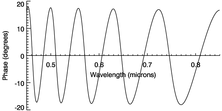
The instrumental phase term can be measured by observing a calibrator star (which has zero source phase). The observed phase of a calibrator may contain both instrumental and atmospheric phase terms, which is not a problem because the phase terms are additive. Figure 1 shows the measured phase of a calibrator star. The atmospheric phase term takes the form

\theta_{\text{atm}}=\frac{2\pi}{\lambda}\left[v+\left(n-1\right)a\right]+\phi

(3)

where $v$ is a vacuum path, $a$ is the atmosphere path, $n$ is the wavelength-dependent index of refraction, and $\phi$ is a phase offset.

Refer to caption — Figure 1: The phase of a calibrator star. This is the sum of the instrumental phase and some atmospheric phase.

We can then measure the brightness ratio and separation vector by fitting equation 2 to the baseline phases, with equation 1 inserted for the source phase, and equation 3 inserted for the atmospheric phase term. Note that the binary phase term in equation 1 is monotonic as it stands, but in a typical measurement we will see the phase be roughly centered around zero. This is because the fringe-tracker of the interferometer will add the appropriate vacuum delay to give the fringe close to zero phase. Figure 2 shows an example of what the phase of a binary might realistically look like in at high spectral resolution in a fringe-tracking instrument interferometer like the NPOI[2].

3 Data sets

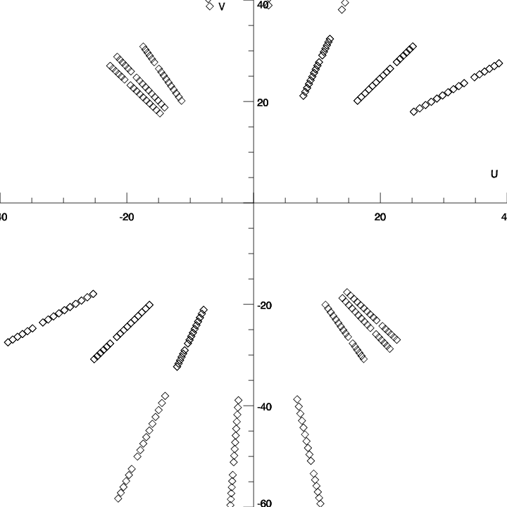
We will present measurements of two stars, $\theta^{2}\,\text{Tauri}$ and $\kappa\,\text{Ursa Majoris}$ observed on the same night. On that night the NPOI was configured to observe three baselines, one of which was observed on two spectrographs. Table 1 lists the target observations. In addition to target observations there were several calibrator observations to measure the instrumental phase for subtraction.

Date Time (UT) Target Hour angle 2004/1/30 04:43 $\theta^{2}\,\text{Tau}$ 1.373 2004/1/30 06:09 $\theta^{2}\,\text{Tau}$ 2.810 2004/1/30 07:15 $\theta^{2}\,\text{Tau}$ 3.923 2004/1/30 06:37 $\kappa\,\text{UMa}$ -1.284 2004/1/30 09:31 $\kappa\,\text{UMa}$ 1.612 2004/1/30 10;26 $\kappa\,\text{UMa}$ 2.499 2004/1/30 10:47 $\kappa\,\text{UMa}$ 2.871 2004/1/30 11:26 $\kappa\,\text{UMa}$ 3.541

Table 1: Observations of

\theta^{2}\,\text{Tauri}

. All observations lasted

30\,\text{s}

4 Analysis

The coherently integrated visibilities are produced using the methodology presented in the paper [1] in these proceedings. The fit of the functional form of equation 2 is not trivial. There are many false minimas such that it is important to either use a minimization method which finds the global minimum and ignores local minima, or to give the minimization procedure an initial guess which is within the capture region of the global minimum. In this paper we are taking the second approach and use a grid-search to obtain an approximate initial guess. If we examine equations 2, 3, and 1 we note that there are three parameters for the binary, $r$ (brightness ratio), $\alpha$ , and $\beta$ (separation along the $u-$ and $v$ -axes respectively). In addition, there are three parameters for each baseline, $v$ , $a$ , and $\phi$ . For $N$ baselines there are thus $3\times\left(N+1\right)$ parameters, and it is not feasible to do a grid search over that many parameters. Fortunately, the coherent integration process results in an average phase which is close to zero. If we therefore use a binary phase model which has approximately zero mean phase (we achieve this by adjusting the vacuum path) then we can in many cases reduce the grid search to cover just the parameters $r$ , $\alpha$ , and $\beta$ . If we make a reasonable guess for $r$ from the amplitude of the phase variations then the grid search is reduced to just two parameters.

4.1 $\theta^{2}\,\text{Tauri}$

In the analysis of $\theta^{2}\,\text{Tauri}$ we begin with a grid search as outlined above. Figure 4 shows the goodness of fit as a function of the two separation parameters. We chose a brightness ratio of $r=0.35$ based on examining the amplitude of the phase oscillations in the raw data. The grayscale of the figure indicates the goodness of fit according to a $\chi^{2}$ metric, with a brighter color indicating a better fit and a darker color indicating a worse fit. The best fit, at $\alpha\approx 20\,\text{mas}$ , and $\beta\approx 20\,\text{mas}$ is framed by two white diamonds. Notice that there is also a good fit (but not quite as good) at approximately $(-\alpha,-\beta)$ . Finally, notice the complexity of the fitness landscape. Without a good initial guess or a optimization method which is able to ignore local minima it would be unlikely that the fit converges on the global minimum.

Using this initial guess we then fit the full function (Equation 2 with equations 1, and 3 inserted) to the 12 baseline measurements simultaneously (i.e. using the same binary star parameters for every baseline). However, we make one modification in that we allow $r$ to vary linearly with wavelength. We then obtain the fit shown in figure 5. In this figure the solid curve shows the baseline phase (including error bars which are often too small to distinguish), and the dotted curve shows the best-fit model.

In order to estimate the uncertainty on the fitted parameters, $r$ , $\frac{dr}{d\lambda}$ , $\alpha$ , and $\beta$ , we perform a bootstrap Monte Carlo analysis. Bootstrap error analysis is a simple way of estimating the sampling uncertainty from a data set with the same distribution as the measured data set. It proceeds by repeatedly selecting $N$ (with replacement) from the $N$ independent segment of the data set and performing the full analysis to obtain parameters, each time obtaining a slightly different set of parameters. If the data set is a good representation of the distribution from which it is taken (this is the usual assumption) then the distribution of parameters represents the uncertainty of such a sample. We took 100 bootstrap samples and arrived at separation parameters of $\alpha=17.134\pm 0.033\,\text{mas}$ , $\beta=17.989\pm 0.022\,\text{mas}$ , which yields a precision on the separation of approximately $0.16\%$ . The brightness ratio as a function of wavelength is plotted in Figure 6. In that figure the solid curve is the brightness ratio, whereas the dotted curves represent one standard deviation. Also plotted are measurements of the brightness ratio from Armstrong et al. (2006) [3]. That paper used a much larger database than the present work, spanning both Mark III and NPOI data, yet arrived at uncertainties in the brightness ratio which are similar to or greater than ours. Table 2 lists the brightness ratio at several wavelengths. The discrepancy between this work and prior work will elaborated on in the discussion section. For now we just note that the reduced $\chi^{2}$ of the fit is approximately eight, corresponding to a mean difference between model and data of 2.5 standard deviations.

$\lambda\,(\mu\text{m})$	This work	Armstrong et al. (2006)
0.50		$1.05\pm 0.05$
0.55	$1.03\pm 0.03$	$1.12\pm 0.03$
0.65	$1.08\pm 0.02$
0.70	$1.10\pm 0.01$	$1.16\pm 0.03$
0.75	$1.13\pm 0.01$
0.80	$1.16\pm 0.01$	$1.14\pm 0.05$

Table 2: Brightness ratio as a function of wavelength for this work compared with Armstrong et al. (2006)

4.2 $\kappa\,\text{Ursa Majoris}$

The second example, $\kappa\,\text{Ursa Majoris}$ is more challenging. It consists of five observations on the same set of baselines. We approach this data set in the same way as the previous data set, and the final fit to the data is presented in Figure 7. The fit corresponds to a brightness ratio of $\Delta M\approx 0.5$ , and separation $\alpha=-115\,\text{mas}$ , $\beta=85\,\text{mas}$ . Because of discrepancies between the model and the data we do not specify uncertainties but instead refer to the discussion section.

5 Discussion

An important consideration when doing high-accuracy work is knowledge of the wavelengths to a high degree of accuracy. In the case of $\theta^{2}\,\text{Tauri}$ wavelength knowledge is less critical for estimating the brightness ratio, but still important for the separation. In the case of a large-separation binary system such as $\kappa\,\text{Ursa Major}$ it is much more important. For both the data sets analyzed here only nominal wavelength and bandpass information was available, and that likely is a contributing factor to the imperfect fit $\chi^{2}=8$ in the case of $\theta^{2}\,\text{Tauri}$ and is probably the dominant effect of the goodness of the fit in the case of $\kappa\,\text{Ursa Major}$ . In Figure 7, panels (b) and (d) contain the same baseline, but recorded on two different spectrographs. However the two observations are not identical, which is especially evident at the blue end of the spectrum. The likely cause of this is that the two spectrographs have slightly different wavelength scales. We are not able to correct this effect because no measured wavelength information was available for that particular date. However on later dates the bandpass is measured to a high degree of accuracy.

Another important thing to notice, if we look at Figure 6, is the discrepancy between the present results and those of Armstrong et al. (2006)[3]. First, in the older data we observe what appears to be a curvature as a function of wavelength. We do not see this in our data because we modeled the brightness ratio to be linear with wavelength. It would be interesting to add a quadratic term and then repeat the comparison. Another thing to note is that Armstrong et al. (2006) obtain slightly larger brightness ratios than us. It is important to realize in this context that the amplitude of the phase oscillation is modulated not only by the brightness ratio, but also by the visibility amplitude of the component stars. The component stars are unresolved such that visibilities are close to one. We did not take that effect into account in this initial work.

6 Conclusion

We have demonstrated that coherently integrated visibility phases can be used to obtain high-quality measurements of the fundamental parameters of binary stars. The measurements are accurate to the point where careful calibration of wavelengths and bandpasses is necessary. This calibration was not available for the data sets considered in this paper, but is routinely performed on more recent NPOI data sets.

Acknowledgements.

The NPOI is funded by the Office of Naval Research and the Oceanographer of the Navy. The authors would like to thank R. Zavala for useful suggestions and for help with access to the relevant data.

References

[1] A. M. Jorgensen, D. Mozurkewich, H. Schmitt, R. Hindsley, J. T. Armstrong, T. A. Pauls, and D. Hutter, “Practical coherent integration with the npoi,” Proceedings of the SPIE Astronomical Telescopes and Instrumentation (This volume) , 2008.
[2] J. T. Armstrong, D. Mozurkewich, L. J. Rickard, D. J. Hutter, J. A. Benson, P. F. Bowers, N. M. Elias II, C. A. Hummel, K. J. Johnston, D. F. Buscher, J. H. Clark III, L. Ha, L.-C. Ling, N. M. White, and R. S. Simon, “The Navy Prototype Optical Interferometer,” Astrophys. J. 496, pp. 550–571, 1998.
[3] J. T. Armstrong, D. Mozurkewich, A. R. Hajian, K. J. Johnston, R. N. Thessin, D. M. Peterson, C. A. Hummel, and G. C. Gilbreath, “The Hyeades binary $\theta^{2}$ Tauri: confronting evolutionary models with optical interferometry,” AJ 131, pp. 2643–2651, 2006.