year number number identifier Date: ]August 24, 2026
Optical spectra of a quantum dot in a microcavity in the nonlinear regime
Abstract
The optical emission spectrum of a quantum dot in strong coupling with the single mode of a microcavity is obtained in the nonlinear regime. We study how exciton-exciton interactions alter the emission spectrum of the system, bringing the linear Rabi doublet into a multiplet structure that is strongly dependent on the cavity-exciton energy detuning. We emphasise how nonlinearity can be used to evidence the genuine quantum nature of the coupling by producing satellites peaks of the Rabi doublet that originate from the quantized energy levels of the interactions.
I Introduction
Since the first experimental realization of atomic cavity quantum electrodynamics (cQED),[1] a wealth of new results have been obtained in the physics of strong coupling of a zero dimensional quantum system to a single photon mode.[2, 3, 4, 5, 6] The problem is important not only because of the fundamental aspects brought forward by the interaction of material systems with photons,[7] but also because of the potential application of cQED to quantum information processing.[8, 9] In semiconductors, strong coupling is routinely achieved in planar microcavities—where in-plane excitons couple to photons with matching momenta—since the phenomenon was experimentally evidenced in 1992.[10] Strong coupling in 2D now provides the basis for investigating exotic phases of matter in these structures such as Bose-Einstein condensates[11, 12, 13, 14] or superfluids.[15, 16, 17, 18] One system that has recently attracted particular attention is the zero-dimensional analog that consists of a Quantum Dot (QD) coupled to a single microcavity mode.[19, 20, 21, 22, 23] The material excitations in the QD are excitons, that is, bound electron-hole pairs. Owing to their spatial confinement and energy level discretization, they can be brought in strong coupling with the single mode of a microcavity, such as that offered by a pillar (etched planar cavity),[20] the defect of a photonic crystal[21] or the whispering gallery mode of a microdisk,[22, 23] among others. In Refs. [20, 21, 22], such structures have demonstrated the Rabi doublet in their optical spectra, which is characteristic of the mode anticrossing that marks the overcome of dissipation by the coherent exciton-photon interaction.
Steady progress is being made towards a better quantum strong-coupling as well as towards its external control. Passive photonic crystals with breathtaking values of have now been reported,[24] limited only by structural imperfections. As the fabrication process will improve, a gain of another order of magnitude in the quality factor is allowed by the available theoretical designs. As for the active element, which inclusion lowers the quality factor, prowess have been achieved in the engineering of the heterostructure allowing to deterministically position a QD inside a photonic crystal to within 25nm accuracy, and thus place the dot at a maxima of the light intensity, along with an etching technique of the holes of the photonic crystal to match spectrally the QD and cavity mode emission.[25] Micropillars etched out of Bragg mirrors allow a fine control of the radius and even of the shape of the cross-section, that can be optimised to reach high values of the quality factor, with figures of reported for radius size of m.[26] One appealing feature of these structures is their ease of access both for the excitation and the emission, the latter being perpendicular to the sample surface. The mode volume in these structures can be further reduced while maintening the quality factor in one polarization by using elliptical pillars, and record values of can be achieved in this way.[27] At the same time, the density of self-assembled QDs in the active medium has been successfully reduced over the years, with figures of cm-2, and the possibility to grow large dots (with lens shape of nm) so as to provide a large oscillator strength. With microdisk resonators, the whispering gallery modes of a thin disk supported by a column provide the high modes of the cavity.
These milestones open the way to new research investigating the “true” quantum nature of the exciton-photon coupling.[28] Although the system exhibits strong coupling, it is not known in which quantum state it is actually realized. To be useful for quantum information, the system must deal with few quanta of excitation and display strong alterations of its characteristic for small changes in particle number populations. If the system scales linearly with the number of particles, it is essentially classical,[29] and adding or removing a single particle will not change its behaviour. Therefore, probing the nonlinear response is desirable. Recently, in an attempt to validate the single-particle character of the Rabi doublet in a QD-microcavity system, an unexpected additional peak was observed that was attributed to renormalisation of the exciton energy by charging centres close to the QD.[30] The observed antibunching allowed the authors of Ref. [30] to confirm the quantum character of this coupling, but much is left to understand of the nonlinear effects and the nature of the additional peaks, observed or predicted.
In this text, we compute the spectra of emission for a pumping high enough to enter the nonlinear regime. With QDs in microcavities, two types of strong nonlinearities are expected,[31] both associated to the active material, i.e., the excitons. The first one comes from Coulomb repulsion of the charged particles, and is the one investigated here, in the case where it is comparable to the coupling strength. The other comes from Pauli exclusion, that arises from the fermionic character of the underlying particles.[32] In Refs. [31, 33], the effect of Pauli exclusion alone was investigated (Coulomb interactions were added in an as yet unpublished work.[34]) There it was shown that Pauli exclusion resulted in rich multiplet structures depending on the size of the dot, with a Mollow triplet-like structure for small dot with strong Pauli repulsion, and a Rabi doublet for large dots. In the present work, we show that even for bosonic excitons, a multiplet structure arises in the emission spectrum when intra-dot exciton-exciton interaction is accounted for. For the large dots that the model aims to describe, Pauli exclusion can be taken into account phenomenologically by a phase-space filling effect that screens the exciton-photon interaction.[35, 36, 37] The latter results in loss of strong-coupling and we therefore focus on the intermediate regime where such renormalization of the coupling strength can be neglected. We also neglect the spin-degree of freedom, in particular the sign-dependent interaction between same and opposite-spins excitons, respectively.[38] This allows us to focus on nonlinear deviations and to neglect more complicated correlations effects of the multi-excitons complexes such as formations of bound pairs or molecules that would give rise to bipolaritons.[39, 40, 41] Experimentally, this could be realized by using a circularly polarised pump. Strong qualitative changes are still observed, with a basic structure that consists of a blueshifted peak on top of a distorted Rabi doublet.
The paper is organised as follow. In Sec. II, we introduce the Hamiltonian of the system describing the coupling between cavity photons and interacting QD excitons. From this Hamiltonian, we extract the energy level structure. This already contains the essential information to understand qualitatively the spectra that we compute through more refined methods in the next section. In Sec. III, we use the density matrix formalism and solve the master equation in the steady state to compute the spectra using the quantum regression theorem. This method, which suffers in principle no limitation or approximation (beyond assuming Markovian dynamics), can only be used in practice for the low pumping regime, as the computational cost goes like with the method that we use here, where is the truncation order (the maximum number of photons accounted for in the model). We also propose an alternative formalism for the calculation of the emission spectra based on the Keldysh Green function technique and compare the results obtained by the two methods. In Sec. IV, we discuss the overall results and conclude. The Appendix contains the mathematical details of the calculation of the emission spectra using the Keldysh Green function technique.
II Model Hamiltonian
We describe light-matter interaction in a large QD including exciton-exciton interactions with the following Hamiltonian:
| (1) |
The operator () is the annihilation (creation) operator for the cavity photon () and QD exciton (). They all follow Bose algebra. The parameter is the coupling strength and accounts for the exciton-exciton interaction. In all the following, is taken as the unit. An important parameter of the system is the detuning . The reference energy is that of the exciton, that is set to zero, . In eqn (1), we neglected the polarization degree of freedom,[42] thus addressing the case of a symmetric QD under normal excitation, or excited by a circularly polarised light.
To obtain an intuitive picture on the optical spectrum of such a system, we first study the allowed transitions between the possible energy levels. That is, we first obtain the eigenstates of the system with excitations by diagonalizing the Hamiltonian (1). Note that the total number of excitations is conserved. In what follows, we refer to the set of eigenstates of the total particle number with eigenvalue as the th manifold of the system.

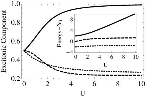
The structure of energy levels at resonance is sketched in Fig. (1) up to a maximum of two excitations (i.e., up to the second manifold) for three different cases. First, the bare levels corresponding to non-interacting and uncoupled (or weakly-coupled) modes (, ). Second, the eigenenergies arising from the coupling (, ), and finally, the blueshifted lines that result from including the interactions (, ). All the levels but those in the manifold , involving only one particle, change with the interactions because of the excitonic part of their corresponding eigenvectors. In order to keep track of the excitonic character of each level, in Fig. (2), we plot the excitonic component of the eigenvectors of manifold and their corresponding eigenenergies as a function of the interaction . We can see that, starting from a situation completely symmetric between the photonic and excitonic fractions, the higher level gets more and more excitonic-like with and blueshifts strongly. The other two energy levels are only slightly affected, as follows from their more photonic character. This characterisation of the levels, which also depends on the detuning, plays an important role when identifying the spectral lines, as we show in the following sections.
The energy levels of Fig. (1) are broadened by the finite lifetime and by the incoherent pumping mechanism. This will be taken into account accurately in Section III. At this stage, an imaginary part is added to the energies of the bare states of the Hamiltonian (1). This is justified a posteriori by comparison with an exact numerical method.
Once computed the new complex eigenvectors and eigenenergies, we obtain the amplitudes of probabilities of loosing an excitation from a given manifold to the neighbouring one counting one excitation less. We consider the amplitude for the processes of annihilation of a photon, that is, the transitions corresponding to the normal mode emission. If the coupling is strong enough, the optical spectrum can be approximated as a sum of Lorentzians corresponding to each allowed transition.[43] The emission lines are finally broadened with the sum of the imaginary parts of the eigenstates involved in the transition and weighted by its probability.


These results are plotted for transitions between manifolds with 2 and 1 excitation as a function of the nonlinearity strength on Fig. (3)a and as a function of the detuning on Fig. (3)b. In the latter case, the exciton bare energy is kept constant, equal to zero, while the cavity mode is brought in or out of resonance with the exciton. This relative detuning between the bare exciton and photon is tunable experimentally through a variety of techniques that include changing temperature or applying a magnetic field (shifting the energy of the dot with negligible perturbation on the cavity) to growing a thin film (shifting the cavity mode energy without affecting the dot). As this is a parameter easy to tune experimentally, that brings many and specific changes in the system, a density plot of photoluminescence emission with detuning of the type of Fig. 3 is the kind of results we are aiming for. On such a plot, one can trace the intensity, width and location (that include the number) of spectral lines for smooth changes in the detuning.
Peaks appearing in Fig. (3)a correspond to the transitions plotted in Fig. (1). They are labelled in blue (colour online): lower lines are the transitions “A” and upper lines the transitions “B”. Comparing with the linear Rabi doublet, which is superimposed in red, we observe the aforementioned blueshift of both groups of lines. It is more important for the exciton-like mode (especially line B-2 at resonance when ) while the photon-like mode has a better resolved fine-structure splitting. At various detunings (Fig. (3)b), complicated structures are found with crossing or anticrossing of the lines, as shown on the figure. Lines with the same bare-excitation (photon or exciton) character cross, whereas lines of a different character exhibit anticrossing. At large detunings, the bare photon and exciton modes (in green) are recovered but with an additional blueshifted bare exciton line.
Satellite peaks arise at very low and high energies from transitions that are forbidden in the linear regime. They enter the dynamics through nonlinear channels opened by the interactions. The dashed arrows in the right panel of Fig. (1) represent these two transitions, with two excitons as the initial state that release one excitation and leave one photon as the final state. They appear dimly in Fig. (3).
Thus, the manifold method allows an understanding of the composition of the optical spectra, as illustrated on Fig. (3) where the spectral lines have been labelled according to their corresponding transitions on Fig. (1). From this overall picture, the excitonic fraction is clearly associated to the blueshift. Which transitions enter the dynamical picture, and to what extent, is investigated by the exact dynamical treatment that we pursue in terms of the density matrix formalism.
In the next section, to describe more realistically the experimental situation, we supplement eqn (1) with an external excitation and a decay mechanism for the QD exciton and cavity mode. This is done by supplying a reservoir of external photons coupled to the cavity mode (to account for the finite lifetime of cavity photons) and another one to the exciton mode (to account for the exciton decay into photonic modes other than the cavity). Both pumping and decay compensate and the system reaches a steady state.
III Calculation of the emission spectra
The coupling of the system to the external world results in a leakage of photons and of QD excitations, that imply that even when the initial state of the system is well known (pure state), the system evolves into a mixture of states where only probabilistic information is available. A suitable treatment of such a dynamics involves the density matrix operator . Its temporal evolution is given by a master equation of the type:
| (2) |
with the Hamiltonian dynamics already introduced in eqn (1), and with the incoherent contributions in the form of Lindblad terms , defined as
| (3) |
that corresponds to the general de-excitation operator and its effective decaying rate . Explicitly, the escape of the cavity photons is accounted for by a Lindblad term , with a rate . This parameter is inversely proportional to the cavity quality factor :
| (4) |
The spontaneous decay of the QD excited states into any other mode than the one of the cavity, as well as the non-radiative decay, are taken into account with the term and its associated rate . Such a rate is typically much smaller than the cavity emission rate, . Finally, the cavity or the excitons can be pumped with a continuous incoherent pumping. The associated Lindblad terms now involve the creation operators. The master equation in our system therefore reads:
| (5) |
We have included two possible kinds of incoherent pumping, namely, the cavity pumping at rate and the electronic pumping (via the exciton) at rate . Experimentally, the most common practise is electronic pumping, as the photoluminescence from the cavity is usually observed and pumping it would hinder the measurement. could be taken into account to describe an effective cavity pumping due to, for instance, other dots that are weakly coupled to the cavity modes and populate the cavity with photons [43]. In the case of direct cavity pumping, it would be more relevant to observe the exciton emission for photoluminescence, or to turn to coherent excitation and probe the transmission, reflexion and/or absorption of the cavity. Here we compute the cavity photoluminescence for the two kinds of pumping each considered on their own, for the purpose of comparison, keeping in mind that the more experimentally relevant case is that of electronic pumping.
We first obtain the steady state of the system, by solving .[44] From the knowledge of this density matrix we can compute the mean value in the steady state of a general operator as . More interestingly, the optical spectra of the system can also be obtained from and the master equation (5) thanks to the quantum regression theorem.[45, 46] We write the steady state equation in the matrix form:
| (6) |
where the labels and index the whole Hilbert space, namely, in our case of two oscillators, and . As a result, is a matrix where is the truncation of each oscillator’s Hilbert space. In the computations, we have checked that the results were independent of this truncation once it is taken large enough. The emission spectrum in the steady state, defined as
| (7) |
can then be obtained from Lax’s hypothesis that the two-time correlators follow the same regression equations than the average:
| (8) |
where and are the creation and destruction operators of the transitions and is defined as
| (9) |
that is, in the case of cavity (normal) emission, where and :
| (10) | ||||
| (11) |
The drawback of this method is the high computational cost involved in solving eqn (6) to obtain and to subsequently invert it in eqn (8). Therefore, we present here the spectra for the low pump regime. This is not a serious limitation for the time being, however, as we are primarily interested in small deviations from the linear regime and to probe the first ladders of the quantized energy levels. We use pumping rates of , yielding average number of excitations of the order with probability to have two excitons of the order of . For these figures, a truncation at the fourth manifold () is enough to ensure convergence of the results. The other parameters are fixed to the following values, motivated by experiments: provides the unit (experimental figures are of the order of tens of eV), , and .


Mean numbers of excitons and photons are plotted on Fig. (4), for the two cases of cavity (only) and electronic (only) pumping. Close to resonance, , both pumping yield approximately equal exciton and photon populations (note that the cavity pumping case has been magnified by a factor five). Detuning the modes results in a collapse (cavity pumping) or increase (electronic pumping) of the exciton population, as could be expected. Regardless of the kind of pumping, however, the cavity population is approximately constant. In the cavity pumping case, this is because the exciton gets decoupled and thus the cavity is pumped at a constant rate (one can actually see a small increase in its population). In the electronic pumping case, this is because although the coupling decreases, the exciton population increases in proportion so as to feed the cavity with a constant flux of photons. In both cases, an asymmetry is notable with detuning, because the interactions bring the cavity and the exciton modes closer or further from resonance, respectively, coupling them more efficiently for positive detuning and therefore allowing a larger production of excitons in that case. As a result, the nonlinear branches of the actual spectra (i.e., branches others than the Rabi doublet) for positive and negative detunings, shown on Fig. (5), are not exactly as those shown in Fig. (3)b. The blueshifted peak is more clearly seen in the positive detuning case thanks to this exciton population asymmetry with detuning. However, an excellent qualitative agreement is obtained with the manifold method, if one superimpose the vacuum Rabi doublet to the lines arising from higher manifolds. Depending on the pumping scheme—cavity (a) or exciton (b)—only quantitative features are changed that consist mainly in different linewidths and intensities of the branches, that are otherwise well accounted for by the manifold method (see also Fig. 6). While comparing Figs. 5(a) and (b), it should be borne in mind how the total population changes with detuning, as shown on Fig. 4. For this reason, panel (b) has a more complex structure, but this is due to the higher manifolds that can be reached with the electronic pumping. It is in fact possible to identify the third to second manifold contribution by extracting the lines in Fig. (5) that do not appear in Fig. (3)b. These lines are clearly weaker due to the very low (but not vanishing) probability to have three excitons in the system. The transitions from even higher manifolds are too improbable to be seen in the spectra for the pumping considered here. The main differences between the two pumping schemes, if equal populations can be considered by adjusting the pumping, are therefore to be found in the linewidth and intensities of the lines. The positions of these lines embeds the most precious indications on the physical system.


On Fig. (6), spectra are displayed for particular detunings, in solid black for the case of electronic pumping, and thin red for cavity pumping. The electronic pumping, which we repeat is the most relevant case experimentally, yields the most interesting spectral shape. On top of the Rabi doublet, the interactions produce additional peaks that, at large detunings, are clearly associated to the exciton (panels (a) and (e)). Three peaks, E1, E2 and E3 are obtained that correspond to one, two and three excitons coupling to the cavity mode, respectively. As these are brought in resonance with the cavity mode, the linear Rabi doublet dominates (essentially because the efficient coherent coupling collapses the exciton population) and satellite peaks are observed, that betray the quantum nature of the system, as the emission originates from transitions between quantised manifolds. In the absence of interactions, the Rabi doublet is always observed independently of the total number of particles (this is the definition of a linear behaviour). Therefore, interactions are useful to evidence a quantum behaviour linked to quantized energy transfers, in the spirit of such experiments as those used with atoms in cavity to demonstrate quantization of the light field.[47] Here, nonlinear features are observed directly in the optical spectrum, whereas in Ref. [47], time-resolved measurements were used to probe anharmonic oscillations of the Rabi flops. This represents a notable experimental advantage, as measurements with cw incoherent pumping are typically easier to perform than time-resolved spectroscopy.
We conclude this Section by discussing the computation of the emission spectra in terms of nonequilibrium Green functions, that could be used when the size of the Hilbert space forbids numerical computations with a master equation. Keldysh Green functions are now routinely used in description of electronic transport in mesoscopic systems[48] and we believe that their application for the description of optical properties of QDs in the nonlinear regime is of methodological interest. Besides, this approach allows the discrimination between mean-field and correlation effects, which is important for the understanding of the physical origin of the additional peaks in the spectra of photoemission considered above. It can be shown (see Appendix for details) that within a Hartree-Fock approximation the emission spectra contains of a Rabi doublet and no satellite peaks appear. This corresponds rather well to the case of the planar microcavities with embedded quantum wells where the number of excitations is large, but does not give an adequate description of the spectra of QDs where the total number of excitations in the system is small and correlation effects play a substantial role. Taking them into account within the Keldysh Green function formalism allows to reproduce the multiplet structure of the spectra, as shown in Fig. (7) for the same parameters and occupation numbers as in the case of cavity pumping in Fig. (4) and (5). The Green function results agree with those obtained with the density matrix formalism, the main difference being an anticrossing between the satellite branches clearly seen at Fig. (7), which is probably related to the truncation scheme we use.

IV Conclusions
We have analysed the optical spectra of a QD in strong coupling with the single mode of a microcavity at the onset of the nonlinear regime obtained through an incoherent pumping of either the cavity directly, or of the exciton, with nonvanishing probabilities of more than one excitation. We have considered a large quantum dot dominated by exciton-exciton interactions. Exact dynamical results were obtained with a density matrix master equation and the quantum regression theorem. The Green function technique was also applied to support the results and suggest possible extension to arbitrary high number of excitations.
We showed that a deep physical understanding can be attained by identifying the spectral lines with the transitions between quantised energy levels of the nonlinear Hamiltonian. The spectral shapes observed, that probe the first manifolds of multiple excitations, are accounted mainly by the Coulomb energy shift on top of the linear Rabi coupling, with crossings and anticrossings of the lines with detuning, depending on their opposed (photon and exciton) or identical (photon or exciton) character. The quantitative behaviour of the linewidth and intensities of these lines depends mainly on the dynamics of the system, such as the populations of the bare cavity photons and bare excitons. Electronic pumping of the exciton—the case most commonly realized experimentally as far as external incoherent pumping is concerned—allows to achieve high populations at nonzero detunings thanks to the small exciton lifetime and the reduced effective coupling. The balance of these two factors nevertheless retains an approximately constant cavity population. As a consequence, the optimum experimental configuration to observe nonlinear effects in the photoluminescence spectra is at an intermediate, nonzero detuning, for instance when the detuning is approximately equal to the coupling strength. There is an asymmetry with the sign of the detuning due to the interactions that further helps in characterising the nature of the nonlinearity (e.g., to which extent it comes from the exciton-exciton Coulomb interaction). The presence of satellites with detuning demonstrates emission from quantized manifolds, and as such is a signature of the quantum regime. The spectral drift of these lines with detuning is a useful tool to explicit the exact form of the Hamiltonian that accounts for the exciton nonlinearities.
Acknowledgements
We thank Prof. A. V. Kavokin, Prof. C. Tejedor, Dr. R. T. Pepino and Dr. T. C. H. Liew for useful discussions. This work was supported by Brazilian Ministry of Science and Technology, IBEM (Brazil) and by the Spanish MEC under contracts Consolider-Ingenio2010 CSD2006-0019, MAT2005-01388 and NAN2004-09109-C04-3. I. A. Shelykh acknowledges the support of the grant of President of Russian Federation.
Appendix A Optical spectra with the Keldysh Green function technique
In this Appendix, we present the details of the calculations of the photoemission spectrum with Keldysh Green function technique.
To model the pumping and decay of cavity photons and QD excitons within the Keldysh Green function formalism, one needs to introduce the Hamiltonian of the coupling of the photonic and excitonic fields to the reservoirs of in-coming and out-going external photons and excitonic reservoir. The latter corresponds to the pump of the exciton state and its decay towards the leaky modes of the system. The complete Hamiltonian can be thus represented as a sum of that of eqn (1) and the reservoir Hamiltonian given by
| (12) |
The operator () annihilates (creates) one incoming () or outgoing () free photon outside the cavity, annihilates a photon in a leaky mode, the parameters and are cavity-reservoir and exciton-leaky mode coupling strengths respectively and are the dispersions of the external photons and leaky modes. In the Keldysh formalism, the photon spectral emission [counterpart of eqn (7)] is recast as
| (13) |
where is the lesser Green function in the frequency domain for the photons inside the cavity. In order to calculate the correlator in eqn (13), we define the retarded Green function .[48] The equation of motion of follows directly from the Heisenberg equation for the operators :
| (14) |
where
| (15) |
and
| (16) | |||||
with . The functions
| (17) |
correspond to the retarded Green functions for free particles outside the cavity (ingoing and outgoing photons, and leaky modes). To close eqn (14), one needs the expression for , which involves the third order Green function. The full procedure leads to an infinite set of equations, coupling Green functions of different orders (in a so-called Bogoliubov chain). To close this system, one needs to apply a truncation procedure, factorising Green functions of some given order into products of lower-order correlators. The simplest way to close the Bogoliubov chain is to apply the Hartree-Fock approximation, which consists in breaking the correlator into products of two-operator Green function. More specifically, based on the Wicks theorem, one can apply the following approximations:
However, in the problem considered, this mean-field approximation appears to be too rough. Indeed, in this case the resulting spectra consist of a blue-shifted Rabi doublet without any additional satellites (result not shown).
To take correlation effects into account, in the following, we keep the correlators exact up to the second order. In this case, the equation of motion for reads:
| (18) |
where
| (19) |
and
| (20) |
According to the Wick’s theorem for , the following truncation procedure holds:
| (21) |
Substituting eqn (21) in eqn (18) we obtain a new equation for only,
| (22) |
with . Defining the Green function vector
| (23) |
( is for transpose), eqn (22) can be written in a matrix form
| (24) |
where the vectors are underlined once and matrices twice. The matrix of zero order Green functions is given by
| (25) |
where is the matrix with elements of on its diagonal, zero elsewhere, and is defined according to . The matrix is the sum of two terms, , where
| (26) |
and
| (27) |
Finally, the vector is defined as
| (28) |
The quantities can be computed self-consistently together with the lesser Green function through the expression . For simplicity, here we take as numerical parameters. That is, we substitute the effect of the coupling to external reservoirs for an effective decay added as an imaginary part to the bare cavity energy and to the bare exciton energy . The effect of the pump is partially included by adjusting and to the values calculated in Fig. (4). It is possible to show that the Keldysh-contour-ordered Green function has an equation formally similar to eqn (24).[48] Then, applying analytical continuation rules, we find in the frequency domain the equations for the retarded () and the advanced () Green functions as well as for the lesser () Green function,
| (29) |
and
| (30) | |||||
In order to take into account the finite lifetimes of the exciton and photon modes, a phenomenological broadening was included in the lesser Green function of the free particles, which reads:
| (31) |
where for the first three and for the last three diagonal elements of the matrix .
Finally, we note that the equation for the retarded Green function of the first order can be written in a matrix form in the frequency domain,
while for the lesser Green function of the first order one has
References
- [1] See S. Haroche and D. Kleppner, Phys. Today, 42, 24 (1989), for a review.
- [2] C. J. Hood, M. S. Chapman, T. W. Lynn, and H. J. Kimble, Phys. Rev. Lett. 80, 4157 (1998).
- [3] A. Boca, R. Miller, K. M. Birnbaum, A. D. Boozer, J. McKeever, and H. J. Kimble, Phys. Rev. Lett. 93, 233603 (2004).
- [4] T. Aoki, B. Dayan, E. Wilcut, W. P. Bowen, A. S. Parkins, T. J. Kippenberg, K. J. Vahala, and H. J. Kimble, Nature 443, 671 (2006).
- [5] K. Srinivasan and O. Painter, Nature 450, 862 (2007).
- [6] D. Englund, A. Faraon, I. Fushman, N. Stoltz, P. Petroff, and J. Vučković, Nature 450, 857 (2007).
- [7] H. Mabuchi and A. C. Doherty, Science 298, 1372 (2002).
- [8] A. Ĭmamoḡlu, D. D. Awschalom, G. Burkard, D. P. DiVincenzo, D. Loss, M. Sherwin, and A. Small, Phys. Rev. Lett. 83, 4204 (1999).
- [9] C. H. Bennett and D. P. DiVincenzo, Nature 404, 247 (2000).
- [10] C. Weisbuch, M. Nishioka, A. Ishikawa, and Y. Arakawa, Phys. Rev. Lett. 69, 3314 (1992).
- [11] J. Kasprzak, M. Richard, S. Kundermann, A. Baas, P. Jeambrun, J. M. J. Keeling, F. M. Marchetti, M. H. Szymanska, R. André, J. L. Staehli, et al., Nature 443, 409 (2006).
- [12] R. Balili, V. Hartwell, D. Snoke, L. Pfeiffer, and K. West, Science 316, 1007 (2007).
- [13] F. Brennecke, T. Donner, S. Ritter, T. Bourde, M. Köhl, and T. Esslinger, Nature 450, 268 (2007).
- [14] Y. Colombe, T. Steinmetz, G. Dubois, F. Linke, D. Hunger, and J. Reichel, Nature 450, 272 (2007).
- [15] G. Malpuech, Y. G. Rubo, F. P. Laussy, P. Bigenwald, and A. V. Kavokin, Semicond. Sci. Technol. 18, S395 (2003).
- [16] I. Carusotto and C. Ciuti, Phys. Rev. Lett. 93, 166401 (2004).
- [17] I. A. Shelykh, Y. G. Rubo, G. Malpuech, D. D. Solnyshkov, and A. Kavokin, Phys. Rev. Lett. 97, 066402 (2006).
- [18] A. Amo, D. Sanvitto, D. Ballarini, F. P. Laussy, E. del Valle, M. D. Martin, A. Lemaitre, J. Bloch, D. N. Krizhanovskii, M. S. Skolnick, et al., arXiv:0711.1539 (2007).
- [19] L. C. Andreani, G. Panzarini, and J.-M. Gérard, Phys. Rev. B 60, 13276 (1999).
- [20] J. P. Reithmaier, G. Sek, A. Löffler, C. Hofmann, S. Kuhn, S. Reitzenstein, L. V. Keldysh, V. D. Kulakovskii, T. L. Reinecker, and A. Forchel, Nature 432, 197 (2004).
- [21] T. Yoshie, A. Scherer, J. Heindrickson, G. Khitrova, H. M. Gibbs, G. Rupper, C. Ell, O. B. Shchekin, and D. G. Deppe, Nature 432, 200 (2004).
- [22] E. Peter, P. Senellart, D. Martrou, A. Lemaître, J. Hours, J. M. Gérard, and J. Bloch, Phys. Rev. Lett. 95, 067401 (2005).
- [23] M. A. Kaliteevski, S. Brand, R. A. Abram, A. Kavokin, and L. S. Dang, Phys. Rev. B 75, 233309 (2007).
- [24] S. Noda, M. Fujita, and T. Asano, Nature Photon. 1, 449 (2007).
- [25] A. Badolato, K. Hennessy, M. Atature, J. Dreyser, E. Hu, P. M. Petroff, and A. Ĭmamoḡlu, Science 308, 1158 (2005).
- [26] S. Reitzenstein, C. Hofmann, A. Gorbunov, M. Strauß, S. H. Kwon, C. Schneider, A. Löffler, S. Höfling, M. Kamp, and A. Forchel, Appl. Phys. Lett. 90, 251109 (2007).
- [27] D. M. Whittaker, P. S. S. Guimaraes, D. Sanvitto, H. Vinck, S. Lam, A. Daraei, J. A. Timpson, A. M. Fox, M. S. Skolnick, Y.-L. D. Ho, et al., Appl. Phys. Lett. 90, 161105 (2007).
- [28] G. Khitrova, H. M. Gibbs, M. Kira, S. W. Koch, and A. Scherer, Nature Phys. 2, 81 (2006).
- [29] Y. Zhu, D. J. Gauthier, S. E. Morin, Q. Wu, H. J. Carmichael, and T. W. Mossberg, Phys. Rev. Lett. 64, 2499 (1990).
- [30] K. Hennessy, A. Badolato, M. Winger, D. Gerace, M. Atature, S. Gulde, S. Fălt, E. L. Hu, and A. Ĭmamoḡlu, Nature 445, 896 (2007).
- [31] F. P. Laussy, M. M. Glazov, A. Kavokin, D. M. Whittaker, and G. Malpuech, Phys. Rev. B 73, 115343 (2006).
- [32] M. Combescot and O. Betbeder-Matibet, Phys. Rev. Lett. 93, 016403 (2004).
- [33] F. P. Laussy, A. Kavokin, and G. Malpuech, Solid State Commun. 135, 659 (2005).
- [34] M. Glazov, F. P. Laussy, M. Semina and G. Malpuech, submitted to Phys. Rev. B.
- [35] E. Hanamura, J. Phys. Soc. Jpn. 29, 50 (1970).
- [36] S. Schmitt-Rink, D. S. Chemla, and D. A. B. Miller, Phys. Rev. B 32, 6601 (1985).
- [37] A. Ĭmamoḡlu, Phys. Rev. B 57, 4195R (1998).
- [38] A. Kavokin, J. J. Baumberg, G. Malpuech, and F. P. Laussy, Microcavities (Oxford University Press, 2007).
- [39] A. L. Ivanov, H. Haug, and L. V. Keldysh, Phys. Rep. 296, 237 (1998).
- [40] A. L. Ivanov, P. Borri, W. Langbein, and U. Woggon, Phys. Rev. B 69, 075312 (2004).
- [41] H. Gotoh, H. Kamada, T. Saitoh, H. Ando, and J. Temmyo, Phys. Rev. B 71, 195334 (2005).
- [42] I. A. Shelykh, A. V. Kavokin, and G. Malpuech, Phys. Stat. Sol. B 242, 2271 (2005).
- [43] F. P. Laussy, E. del Valle, and C. Tejedor, To be published in Phys. Rev. Lett. arXiv:0711.1894 (2008).
- [44] E. del Valle, F. P. Laussy, F. Troiani, and C. Tejedor, Phys. Rev. B 76, 235317 (2007).
- [45] J. Eberly and P. W. Milonni, Encyclopedia of physical sciences and technology 11 (1987).
- [46] K. Mølmer and Y. Castin, Quantum and Semicl. Opt. 8, 49 (1996).
- [47] M. Brune, F. Schmidt-Kaler, A. Maali, J. Dreyer, E. Hagley, J. M. Raimond, and S. Haroche, Phys. Rev. Lett. 76, 1800 (1996).
- [48] For a textbook discussion, see H. Haug and A. P. Jauho, Quantum Kinetics in Transport and Optics of Semiconductors, Springer Solid-State Sciences 123 (1996).