Random–Matrix Approach
to RPA equations. I
Abstract
We study the RPA equations in their most general form by taking the matrix elements appearing in the RPA equations as random. This yields either a unitary or an orthogonally invariant random–matrix model that does not appear in the Altland–Zirnbauer classification. The average spectrum of the model is studied with the help of a generalized Pastur equation. Two independent parameters govern the behaviour of the system: The strength of the coupling between positive– and negative–energy states and the distance between the origin and the centers of the two semicircles that describe the average spectrum for , the latter measured in units of the equal radii of the two semicircles. With increasing , positive– and negative–energy states become mixed and ever more of the spectral strength of the positive–energy states is transferred to those at negative energy, and vice versa. The two semicircles are deformed and pulled toward each other. As they begin to overlap, the RPA equations yield non–real eigenvalues: The system becomes unstable. We determine analytically the critical value of the strength for the instability to occur. Several features of the model are illustrated numerically.
Keywords:
Random–matrix theory; Random Phase ApproximationPACS
21.10.-k, 21.60.-n, ,
1 Introduction
Random–matrix theory (RMT), introduced into physics by Wigner in the 1950s, has found an ever increasing range of applications. In particular, it has been widely used to describe spectral fluctuation properties of many–body systems (for a review see Ref. [1]). The main ingredients of RMT are general symmetry properties and the assumption that no state in Hilbert space plays a preferred role. The success of this approach can be ascribed to the fact that many physical systems are rather featureless and to a large extent chaotic [2]. Most theoretical work in many–body systems has, on the other hand, been devoted to non–statistical aspects, in particular to identifying and describing collective features. A prominent example is that of the giant collective states in atomic nuclei. An extreme treatment is that of the so–called schematic model [3]: A special (separable) form of the (residual) interaction is responsible for the collective features and a particular (collective) state plays a distinct role. A widely used many–body approximation scheme used in this context is the Random–Phase Approximation (RPA) first introduced to describe the collective plasma oscillations of an electron gas. The RPA describes the response of the system to a time–dependent field and can be derived, for instance, with the help of a quasi–Boson approximation within the equation–of–motion method [4] or the time–dependent Hartree–Fock equations [5].
This paper is the first of a series of two that are written in an attempt to bridge the gap between the two extremes of a purely statistical (and, thus, “democratic”) and a highly special dynamical description (the interesting features reside in a single state). We define a random–matrix approach to the RPA equations by taking the residual interaction matrix elements appearing in the RPA as random. This may look like an oxymoron: The RPA is designed to describe collective features whereas RMT is fundamentally “democratic”. However, in the second paper of this sequel (Ref. [6], in preparation) collective features will be implemented in our model, and the present study of the RMT approach to RPA equations is a prerequisite for that work. Our paper is not the first to address the interplay between collective features and the background of “chaotic states”, theoretically as well as experimentally (see, for instance, Refs. [7] for Gamow–Teller transitions, Ref. [8] for giant resonances, Ref. [9] for analogue states and Ref. [10] and the literature therein on doorway states) and must be seen in this context. To the best of our knowledge, however, this paper is the first where the problem is addressed within a purely random version of RPA.
Our random–matrix model possesses the symmetry of the RPA equations. We study the average spectrum of the model in the limit of large matrix dimension with the help of a generalized Pastur equation [11] and compare the results with numerical simulations. We are especially interested in the instability of the RPA equations. That instability occurs when one eigenvalue becomes imaginary as we contiuously vary a coupling parameter. We derive a general criterion for the instability to develop. Changes of the coupling parameter cause the system to go through four different “phases”: i) the entire spectrum is on the real axis, ii) one part is on the real axis and the other on the imaginary axis, iii) one part is on the real axis, another on the imaginary axis and a third one in the complex plane, and iv) the entire spectrum is on the imaginary axis. We are not aware of other systems, or models, showing this rich behaviour.
The matrix governing the RPA equations is non–Hermitean and so is, therefore, our random–matrix model. A similar model (but with restrictions that do not allow the eigenvalues to become imaginary) was studied in Ref. [12]. Our model does not belong to the ten canonical Altland–Zirnbauer ensembles (see Ref. [13]). We believe that, quite aside from the RPA equations, our work is of interest as a case study in non–Hermitean random–matrix models.
To make the paper self–contained and to define the notation we start out with a brief resume of the derivation of the RPA equations in Section 2. In Section 3 we review the symmetries of these equations and draw conclusions about the distribution of eigenvalues. In Section 4 the random–matrix approach to RPA is defined. In Section 5 we derive the equations for the spectral density using the average Green’s function (Pastur equations). In Sections 6 and 7 properties of the solutions of the Pastur equations are discussed. These are illustrated in Section 8 with numerical simulations. In Section 9 we establish the critical value of the coupling strength at which instabilities occur. Summary and conclusions are given in Section 10. A technical detail is deferred to the Appendix.
2 RPA Equations
For the sake of completeness, we briefly recall the derivation of the RPA equations for particle-hole pairs of Fermions. The derivation uses the equations–of–motion approach. We follow Rowe’s book [4]. It is essentially assumed that pairs of Fermions can approximately be considered as Bosons.
We thus consider Bosonic single–particle states with creation operators and annihilation operators where . These fulfill the commutation relations
| (1) |
We write the Hamiltonian in a form which does not conserve particle number and which is fully analogous to the Hartree–Fock–BCS Hamiltonian for Fermions,
| (2) |
The matrices and both have dimension . For the matrices and we consider two options. The matrix may be Hermitean or real symmetric. Since the s commute, the matrix is symmetric and either complex or real. Thus,
| (3) |
We observe that for Fermions, in Eq. (2) would be antisymmetric. Let denote the ground state of the Hamiltonian in Eq. (2) with energy ,
| (4) |
We postulate that the excited states of the system are created by applying the operators
| (5) |
to the ground state ,
| (6) |
Multiplying Eq. (4) with and subtracting the result from Eq. (6) we get
| (7) |
The ground state is assumed to be annihilated by the operators and by the operators
| (8) |
obtained by arbitrary variations of the ,
| (9) |
Multiplication of Eq. (7) from the left by and use of Eq. (9) yields
| (10) |
Working out the commutators, using the fact that the coefficients and are completely arbitrary, and using the first of Eqs. (3), we obtain
| (11) |
We have defined
| (12) |
and
| (13) |
Eqs. (11) to (13) are the RPA equations for Fermionic particle–hole pairs. Except for one important difference these equations look very similar to the Hartree–Fock–BCS equations for Fermions: The matrix is symmetric while in the BCS case, the pairing potential is antisymmetric. As a consequence the BCS Hamiltonian is Hermitean while the matrix in Eq. (12) is not. This is why the 2N 2N matrix does not belong to one of the symmetry classes studied in Ref. [13].
3 Spectral Properties
Since the RPA matrix is not Hermitean, the eigenvalues need not be real. We investigate some of the consequences.
The matrix in Eq. (12) has the following two symmetry properties. With the unit matrix in dimensions and
| (14) |
we have
| (15) |
Let be an eigenvalue and be an eigenfunction of the RPA matrix,
| (16) |
From the first of Eqs. (15) and it follows that () is also an eigenvalue with eigenfunction . From the second of Eqs. (15) and it follows that is also an eigenvalue with left eigenfunction . We conclude that with also , and are eigenvalues of the RPA matrix . In other words, real and purely imaginary eigenvalues come in pairs with opposite signs, while fully complex eigenvalues with and come in quartets that are symmetric with respect to both the real and the imaginay energy axis.
For the matrix is Hermitean or real symmetric. Then the eigenvalues of are real and appear in pairs with opposite signs. While level repulsion is the hallmark of a Hermitean Hamiltonian, we show that the non–Hermitean part of leads to repulsion (attraction) of levels with the same (opposite) signs, respectively. With increasing strength of level attraction leads to coalescence of pairs of eigenvalues with opposite signs at energy . Coalescence is a signal for the instability of the RPA approach. With a further increase of the strength of the two coalesced eigenvalues leave the point in opposite directions along the imaginary –axis. On the imaginary axis, a pair of eigenvalues may coalesce again and then move away from the imaginary axis in opposite directions along a line that is parallel to the real –axis. Because of the symmetry of the RPA matrix, such behavior must occur in parallel on the positive and on the negative imaginary axis.
Before giving the general argument, we demonstrate these statements using two simple examples. To be specific we consider the unitary case. First, we take and label the matrix elements in an obvious way by and , respectively. Here is real and is complex. The eigenvalue equation is quadratic with the two solutions . Increasing the value of , we pull the two eigenvalues toward each other. The two eigenvalues coalesce at for and become purely imaginary for . Second, we take . We assume that has been diagonalized with eigenvalues and where, in the spirit of the RPA, we assume . The complex matrix elements of are labelled in an obvious way. The secular equation is
| (17) |
which we write in the form
| (18) |
Here , , , and the last part of Eq. (18) defines . This quadratic equation for has the solutions
| (19) |
The argument of the square root vanishes for
| (20) |
while two eigenvalues coincide at if
| (21) |
By definition we have , , and . Inspection shows that also . As we turn on the coupling matrix , , and grow monotonically from zero, and the condition (21) is met prior to condition (20). This shows that the smaller of the two positive eigenvalues coalesces with its negative counterpart at zero (and becomes imaginary) without the two positive (or the two negative) eigenvalues ever coalescing.
We show that coalescence of two eigenvalues of opposite signs at (without coalescence of pairs of positive or pairs of negative eigenvalues) is a general property of the RPA equations. We denote the orthogonal projectors onto the two –dimensional subspaces appearing explicitly on the right–hand side of Eq. (12) by and , respectively. With the energy, we eliminate the subspace with projector at the expense of introducing into the first subspace the effective Hamiltonian . The term added to is a Hermitean (or a real symmetric) operator and, thus, causes level repulsion between the eigenvalues of which, therefore, cannot coalesce as the matrix elements of increase in magnitude. (The non–Hermiticity of the matrix leads to the negative sign of the term , while a Hermitean would have given a positive sign. But level repulsion is independent of the signs of the matrix elements connecting the states). Going to the eigenvalue representation of the matrix and assuming that all eigenvalues are positive, we find that the trace of is negative for all and largest for . This shows that with increasing strength of the center of the spectrum of the positive eigenvalues is shifted towards smaller values, the shift being strongest for the levels near . We conclude that the interaction described by causes level attraction between the eigenvalues of and those of while it causes level repulsion amongst the eigenvalues of and amongst those of .
To investigate the coalescence of eigenvalues at we follow Kato’s book [15]. We denote by the matrix obtained from by the replacement . We assume that the eigenvalues of are all positive. We consider the characteristic polynomial for complex values of . The following statements follow directly from Chapter II.1 of Ref. [15]: The roots of the equation are branches of analytic functions of with only algebraic singularities. At the point where two or more eigenvalues coalesce two eigenvalues assume the common value if the two equations
| (22) |
and
| (23) |
are both fulfilled. For three or more eigenvalues to coalesce, further equations involving higher derivatives of must also be fulfilled. Such equations impose constraints on . Therefore, the generic case is the coalescence of two eigenvalues. (This is a generalization [16] of the Wigner–von Neumann non–crossing rule for eigenvalues). We confine ourselves to that case. Two eigenvalues coalescing at generically possess a square–root branch point at (the case where the two coalescing eigenvalues are holomorphic at also leads to constraints on , is non–generic and, thus, likewise excluded [16]). The same argument applies to the coalescence of eigenvalues on the positive and on the negative imaginary –axis.
The behavior of two coalescing eigenvalues was already studied in the simplest case introduced above. Both eigenvalues are real and have opposite signs for and are purely imaginary and have opposite signs for . With increasing real the two eigenvalues move along the real axis towards each other until they coalesce at . As increases further, the two eigenvalues leave the point zero and move along the imaginary axis in opposite directions.
That behavior is not confined to the case but represents the generic situation. We consider a point of coalescence with real where the two coalescing eigenvalues (denoted by and ) both have the value zero. We assume that for real and , () is positive (negative, respectively). For in the vicinity of we therefore must have
| (24) |
where is some positive constant. Eq. (24) shows that while () is positive (negative) for real and , both and are purely imaginary and carry opposite signs for real and .
The case of two eigenvalues coalescing on the imaginary axis is similar. With the critical strength for coalescence at with purely imaginary, the two eigenvalues are purely imaginary for . Therefore, Eq. (24) takes the form where is purely imaginary. It follows that for the two eigenvalues leave the imaginary axis in opposite directions along a straight line that runs parallel to the real –axis.
4 Random–Matrix Approach
In order to study the generic properties of the RPA equations, we consider a Gaussian random–matrix model. In Fermionic systems, the RPA equations (11) to (13) account for the particle–hole interaction. As that interaction tends to zero, the matrix vanishes while the matrix tends to a diagonal matrix with elements given by the single–particle energies of the particle–hole pairs. We assume that all these energies have the same value which we denote by . In the nuclear case we have where is the frequency of the harmonic–oscillator potential. We write in the form
| (25) |
The Hermitean (or real symmetric) N–dimensional matrix and the complex (or real) symmetric matrix represent the particle–hole interaction. We assume to be a member of the Gaussian unitary ensemble (GUE) or of the Gaussian orthogonal ensemble (GOE), as the case may be. The matrix elements are complex or real Gaussian–distributed random variables with mean values zero and second moments given by
| (26) |
The indices run from to . The angular brackets denote the ensemble average. For , the average GUE and GOE level densities have the shape of a semicircle with radius . The GUE (GOE) is invariant under unitary (orthogonal) transformations () where (, respectively). The elements of are assumed to be Gaussian–distributed random variables with zero mean values and second moments
| (27) |
The ensemble of matrices is invariant under the transformations where and where denotes the transpose. The elements of and of are assumed to be uncorrelated. The spectrum of is expected to be real as long as the matrix elements of are not too large. This is why we parametrized the Gaussian distribution of in terms of an extra parameter . We simplify the presentation by considering only the unitary case in the sequel. The orthogonal case is obtained with a slight change of notation; our conclusions apply to both cases.
It is useful to display the statistical properties of and of in some detail. Writing the elements of the matrix in the form
| (28) |
we note that is real symmetric and is real antisymmetric. The elements of and of are uncorrelated Gaussian–distributed random variables with zero mean value and second moments given by
| (29) |
Similarly, writing the elements of the matrix as
| (30) |
we note that both and are real symmetric. The elements of and of are uncorrelated Gaussian–distributed random variables with zero mean value and second moments given by
| (31) |
With these definitions, the RPA matrix takes the form
| (32) | |||||
We refer to the joint invariance properties of and as to “generalized unitary invariance” (“generalized orthogonal invariance”, respectively). The generalized unitary invariance says that the ensemble of matrices is invariant under the transformation
| (33) |
It was mentioned already that since is not Hermitean, the random–matrix ensemble constructed above does not belong to one of the classes listed in Ref. [Alt]. Non–Hermitean or Non–Cartan random–matrix models have recently received some attention, see Refs. [14, 17]. It seems that our model appears in Table 7 of Ref. [14] as class 21b (lower sign). We are not aware, however, of any detailed analysis of the model.
We study our random–matrix models in the limit . In that limit, the parameter disappears, and each of our random–matrix models is characterized by two parameters. We introduce the first by noting that for the average spectrum consists of two semicircles. Each of these has radius . We measure all energies in units of that radius. The first parameter is then the distance of the center of each semicircle from the origin at . The second parameter measures the strength of the matrix in units of the strength of the matrix , see Eqs. (26) and (27). It is given by
| (34) |
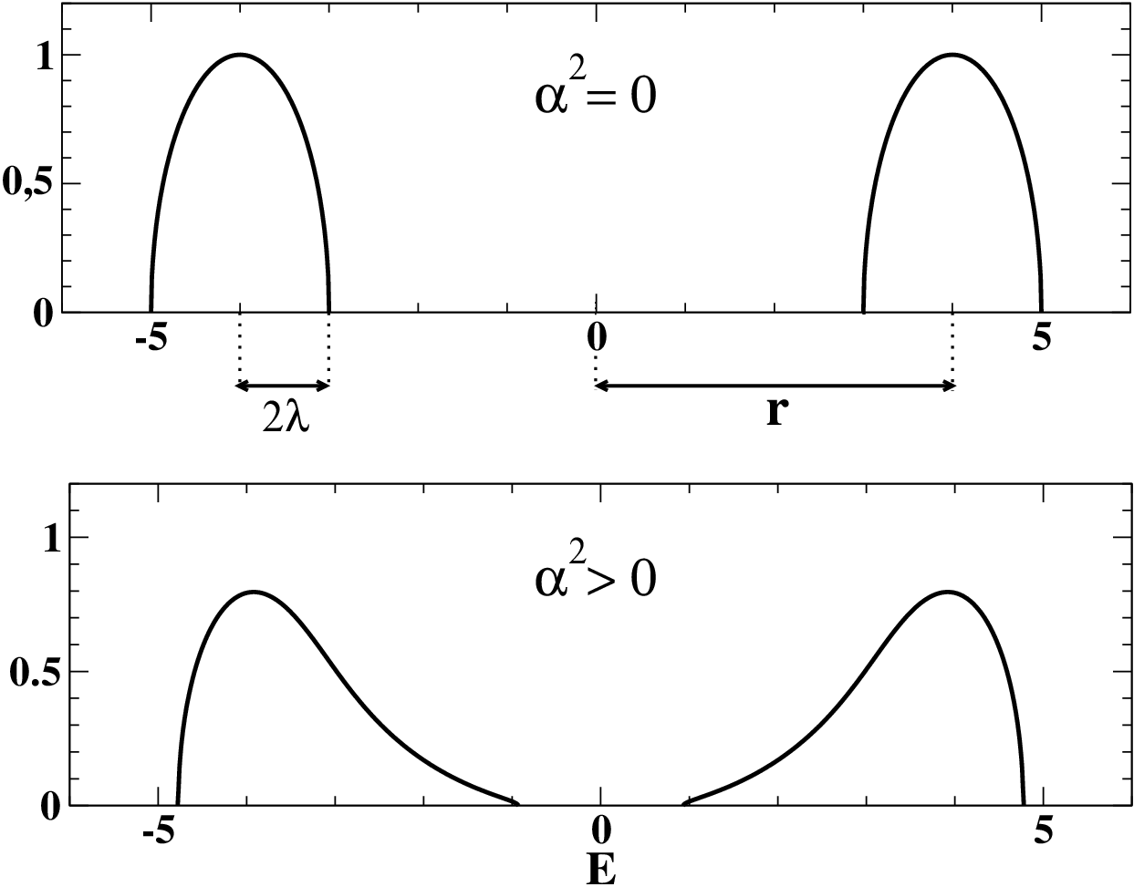
We will use these parameters when we treat the Pastur equation. Using the results of Section 3 we anticipate that with increasing , the two branches of the average spectrum are deformed and move toward each other. This is indicated schematically in Fig. 1.
The average spectrum of our random–matrix model (32) takes a simple form in two limiting cases. Aside from the simplification encountered for and discussed above, another simplification arises in the opposite extreme case when the spectrum is dominated by the matrix . To see this we put in Eq. (32) , and and write the eigenvalues as . The resulting eigenvalue equation is
| (35) |
That equation possesses chiral symmetry. It is straightforward to derive the Pastur equation and to see that the average spectrum has the shape of a semicircle centered at zero with radius . We conclude that as in the RPA matrix in Eq. (32) increases from zero to very large values, the eigenvalues move from the two semicircles on the real axis onto a single semicircle on the imaginary axis. As they do so, they may intermittently leave both the real and the imaginary –axis and form groups of quartets arranged symmetrically with respect to both these axes. This is exemplified in Fig. 2. For and several values of , we show the distribution of eigenvalues in the complex energy plane. These were obtained by diagonalization of randomly drawn matrices of dimension . We see that before all eigenvalues reach the imaginary axis at , a quartet is formed at . We have found numerous such quartets in other random realizations. Our simulations also suggest that in the unitary case, the semicircle formed for very large values of on the imaginary axis has a gap at . In certain chiral ensembles, the average level density is known [18, 19] to vanish at , and our result probably relates to this fact. We have not followed this up any further.

5 Pastur Equations
We ask: How do the matrix elements of affect the average RPA spectrum? Which is the smallest value of where the average RPA spectrum becomes unstable? We answer these questions by calculating the average retarded Green’s function of the system. It is given by
| (36) |
For sufficiently small values of , we expect the average spectrum of to be real and to consist of two branches, one at positive and one at negative energies. The instability of the RPA occurs when the two branches begin to touch.
To calculate the ensemble average, we expand in powers of . This yields
| (37) |
Here is the Green’s function of the system for ,
| (38) |
For the calculation of the ensemble average of is standard: We average each term in the sum in Eq. (37) separately using Wick contraction. For , we keep in each term only the contributions with the maximum number of free summations over the level indices. The resulting series can be resummed and yields the Pastur equation
| (39) |
Using the same notation as in Section 3, we introduce the orthogonal projection operators , onto the two –dimensional subspaces displayed explicitly on the right–hand side of Eq. (33), with etc. The average Green’s function is written as
| (40) |
The terms with on the right–hand side of Eq. (40) vanish. Indeed, it takes an odd number of matrices and an even number of matrices or an even number of matrices and an odd number of matrices to connect subspaces 1 and 2. The elements of being independent Gaussian random variables with mean values zero, such terms vanish upon averaging. This leaves us with
| (41) |
We project the Pastur equation (39) onto each of the two subspaces, use Eq. (41), observe that commutes with and , and obtain
| (42) | |||||
and
| (43) | |||||
We perform the averages over the matrices and using Eqs. (26) and (27), define for the functions
| (44) |
use that
| (45) |
take the traces of Eqs. (42) and (43) and obtain, using ,
| (46) |
With these equations can be rewritten in the form
| (47) |
These are two coupled quadratic equations in the unknown functions and . We refer to both Eq. (39) and to Eqs. (47) as to the (generalized) Pastur equation(s). A physical interpretation of the functions with is given at the end of Section 6.
6 Properties of
Before averaging, can be expressed in terms of the eigenvalues of . We confine ourselves to sufficiently small values of so that for , the average spectrum of consists of two separate branches, the positive branch with eigenvalues , and the negative branch with eigenvalues . Here, . We have used the symmetries of the spectrum derived in Section 3.
We distinguish the advanced and the retarded Green’s functions by appropriate indices. With where is real and positive infinitesimal, we have
| (48) | |||||
Eq. (48) is standard for Hermitean operators. But is not Hermitean. Therefore, we derive Eq. (48) in the Appendix. Averaging over the ensemble converts the sum over delta functions into the average level density ,
| (49) |
where is normalized such that the integral over all energies yields . It is obvious that
| (50) |
The average level density is a symmetric function of . It differs from zero within two energy intervals, one extending over positive energies with end points, say, and where and the other, extending over negative energies between and .
We use to write in the form
| (51) |
Eq. (51) shows that the analytic function has two branch cuts. The branch cut at positive energy extends from the branch point at to the branch point at . The branch cut at negative energies is the mirror image of the first with respect to the origin. The discontinuity of across the cut is given by
| (52) |
For Hermitean problems, the retarded and the advanced Green’s functions are related by complex conjugation. However, is not Hermitean, and and are not complex conjugates of each other. Inspection of Eqs. (36) and (32) shows that with defined in Eq. (14) we have
| (53) |
As long as the two branches of the spectrum do not touch, the functions and have a simple physical interpretation. That interpretation uses Eq. (44) and the spectral decomposition of given in Eq. (48). We first use the results in Section 3 to conclude that if is a right eigenfunction of with real eigenvalue , then is the left eigenfunction to the same eigenvalue, while and are the right and left eigenfunctions, respectively, to eigenvalue . We assume that the eigenvalues are not degenerate. We expand itself (rather than its trace) in the form of Eq. (48) and project the result onto the subspaces with index or . We use and . This yields
| (54) | |||||
Eqs. (54) show that () measures the total average spectroscopic strength of all states in the subspace with index (with index , respectively). For , () receives non–vanishing contributions from the positive–energy states (the negative–energy states) only. As increases, that situation is expected to change. This is confirmed by our numerical calculations.
The analytic properties of used in the present Section may fail to hold when a finite fraction of eigenvalues (i.e., a fraction of order ) is neither purely real nor purely imaginary. In that case use of the Pastur equations as in the present paper may not give correct results because the Green’s function has other singularities besides branch points, see f.i. Ref. [20].
7 Properties of the Solutions of Eqs. (47)
We are going to use the solutions of Eqs. (47) to determine the average level density of the system. By elimination of , Eqs. (47) can be reduced to an equation of fourth order for , see Eq. (60) below. Thus, Eqs. (47) possess four pairs of solutions . It is neccessary to determine which of these is relevant to our problem and how that solution relates to . We use perturbation theory for small values of and continuity to establish that connection. In order to deal with non–overlapping spectra we take .
We first take . Then Eqs. (47) decay into two uncoupled equations for the unperturbed spectroscopic strenghth . With the equations read
| (55) |
The solutions are
| (56) |
The solutions have square–root singularities (branch points) at . For (), the two branch points are at and at (at and at , respectively). The branch cut extends along the real –axis from to (from to , respectively) and connects the two sheets of the Riemann surface. We define the physical sheet as the one where the imaginary part of is positive when we approach the branch cut from below the real axis. Then the square root carries a negative sign for real and , and for real and . On the second sheet we have for real and . For both solutions, the level density differs from zero only if lies on the branch cut, see Eq. (52). In both cases, the average level density is given by the value of on the physical sheet and has the form of Wigner’s semicircle law .
We now consider the case of small and solve Eqs. (47) perturbatively up to first order in . This yields
| (57) |
We note that the end points of the spectrum are not changed. We would expect that with increasing , the branch points are also shifted. Such a shift is, however, beyond the reach of a straightforward perturbative approach, see the end of this Section. We focus attention on and consider the physical sheet of where for . Because of the symmetry of Eqs. (57) our arguments carry over straightforwardly to . The coupling between states in subspaces 1 and 2 shifts some of the spectroscopic strength of subspace 1 into subspace 2 and, thus, into the interval , and vice versa. Both this gain and the corresponding loss of strength in the first interval are given by the last term in the first of Eqs. (57). The first of Eqs. (54) shows that (whatever choice we make for ) the contributions to from the positive– and from the negative–energy states must have the same signs. We have chosen for . Therefore, in the interval , the imaginary part of given by must be likewise positive. That means that must have a negative sign, or that we must choose to lie on the second sheet. We conclude that must be negative: The physically meaningful solutions of Eqs. (57) are the ones where and carry opposite signs. In the interval , the imaginary part of the last term in the first of Eqs. (57) has the form . Here is positive on the second sheet and grows monotonically with , the positive function is given by the semicirle law and is symmetric about , and is antisymmetric about that point and negative for . It follows that is positive (negative) for (, respectively). Moreover, for equal distances of from the negative part has larger magnitude than the positive one. Aside from its loss to the negative energy interval, the level density in the positive energy interval is shifted toward smaller energies. This was expected, see Section 3. The total balance of all these changes must be zero, and the energy integrals over and must be equal since by definition as long as the two branches of the spectrum do not touch. We have not checked that statement analytically for the terms in Eqs. (57) but have tested our numerical results accordingly, see Section 8.
In summary we have shown that for small we must choose those solutions of Eqs. (44) for which the imaginary parts of and have opposite signs. Using continuity we conclude that this statement applies for all values of . Eqs. (44) being real, the non–real solutions come in complex conjugate pairs. Without loss of generality we can choose the solution for which is positive. For the total level density of the system is then given by
| (58) |
We observe that Eq. (58) and the symmetry of the system imply that vanishes at . This is true even when some of the eigenvalues have moved off the real axis.
To investigate the motion of the branch points due to changing , we use a modified version of perturbation theory. We substitute in the first of Eqs. (47) for the asymptotic value on the second sheet and obtain
| (59) |
Solving this quadratic equation we find for the new branch points and the values and . That shows that both branch points are shifted toward smaller energies as expected.
8 Numerical Results
By elimination of , we obtain from Eq. (47) an equation for . It reads
| (60) |
where
| (61) |
Without loss of generality we put . Equivalently, we go over to dimensionless variables by measuring all energies in units of . Then the semicircles have equal radii of value unity, is, for , the distance between the center of each of the two semicircles and the origin, the strength of the coupling, and the dimensionless energy.
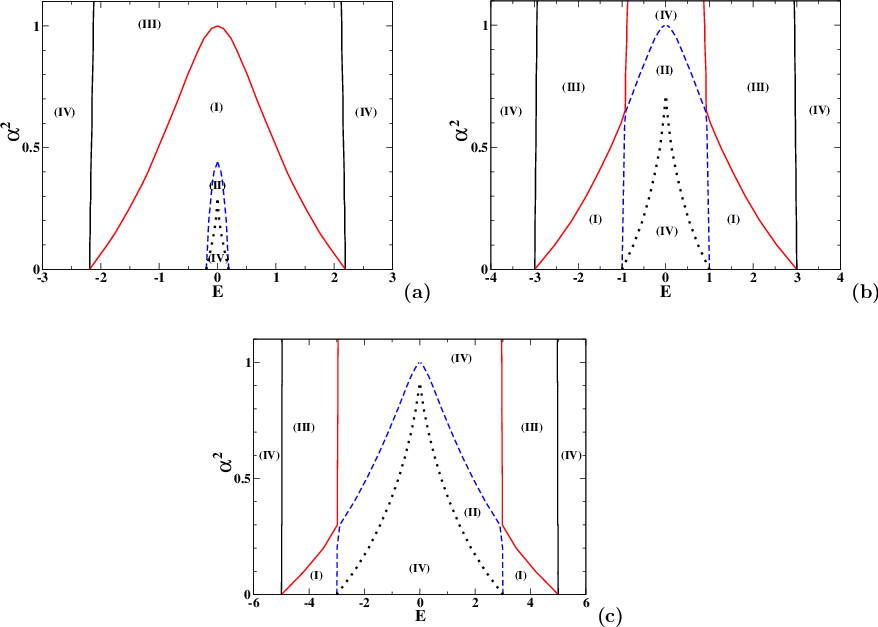
Except for the non–generic cases where the coefficients and are equal to zero, Eq. (60) has four solutions denoted by (). We may either have complex solutions (all four imaginary parts do not vanish identically), or complex and real solutions, or real solutions. Complex solutions always come in complex conjugate pairs. To all four solutions corresponds a unique value of obtained from the first (linear) equation of Eqs. (47). If is real (complex) then is also real (complex). Thus we have the same three possibilities for the pair (, ) : 4 real, 4 complex or 2 real and 2 complex pairs. As explained in Section 7 we look for the complex solution with and . It turns out that that solution occurs for the cases when we have 2 real and 2 complex pairs of solutions, and when we have four complex solutions.
We summarize the properties of the solutions of Eqs. (47) found numerically in Fig. 3. For three values of , we show in the (, ) plane four domains labelled (I) to (IV). These symbols stand for
- •
(I) 4 complex pairs,
- •
(II) 2 real and 2 complex pairs with equal signs for and ,
- •
(III) 2 real and 2 complex pairs with opposite signs for and ,
- •
(IV) 4 real pairs.
The physically interesting solutions lie in domains I and III. In all
three cases shown in Fig. 3, the border lines between domains III
and IV are not vertical but slightly inclined: With increasing
, the spectra are pushed toward . Similarly, the
domains II and IV located at the center become squeezed and finally
disappear. For we only have 4 real solutions (case IV)
or 2 real and 2 complex solutions whose imaginary parts have opposite
signs (case III).
In Fig. 4 we compare for the average level density obtained from the Pastur equation with the actual level density obtained by numerical simulation. We have constructed 100 realizations of the RPA matrix in Eq. (27) with dimension for the unitary case for and three values of by drawing the elements of the matrices and from Gaussian distributions. We have determined the eigenvalues by diagonalization. The results are shown as histograms. The imaginary parts of and are given as dot–dashes and dotted lines, respectively, their sum as a solid line. The very close agreement shows that the Pastur equation is capable of predicting average spectra quite accurately even for matrices of fairly small dimension.


Fig. 5 shows the level density as obtained from Eq. (58) for . For we obtain two semicircles. These are separate for but would overlap for . With increasing , the semicircles become ever more deformed and are pushed towards each other, as expected from the perturbative result in Section 7. Average spectra that are separate for and eventually touch. We observe that the critical value of where this happens (denoted by ) increases with increasing , starting out from at .
In Fig. 6 we show the value of the integral versus . For the integral has the value unity. For the value of should be very close to unity. In that regime, some elements of the matrix for some rare realizations may have large values so that some eigenvalues become non–real and do not contribute to . The resulting decrease of is expected to vanish as , however, and is not visible in Fig. 6. For the value of decreases monotonically with because an ever increasing macroscopic fraction of eigenvalues leaves the real –axis.

9 Critical Strength
The critical strength is defined as the smallest value of for which for two solutions whose imaginary parts carry different signs, and do not vanish at . In order to find an analytical expression for as a function of , we put in Eq. (60) and define, using Eqs. (61), the new variable by
| (62) |
From Eq. (60) we obtain
| (63) |
where
| (64) |
Eq. (63) is an equation of fourth order. The solutions are given by a combination of the three roots of the third–order polynomial ,
| (65) |
The polynomial R(Z) has real coefficients. Therefore, the following possibilities exist.
- •
(i) The three roots of are real and have equal signs; the quartic equation (63) has 4 real solutions.
- •
(ii) The three roots of are real, only two roots have the same signs; the quartic equation (63) has 4 complex solutions.
- •
(iii) Two roots of are complex and one is real; the quartic equation (63) has 2 real and 2 complex solutions.
The roots of are determined via the Cardan method. The substitution
| (66) |
eliminates the quadratic term in Eq. (65) and yields the equation
| (67) |
with
| (68) |
The nature of the roots is determined by the discriminant
| (69) |
If we have case (i), if we have case (ii), and if we have case (iii). Thus, is given by one of the two solutions of . These are
| (70) |
It turns out that () corresponds to the case where the imaginary parts of and have different signs (the same sign, respectively). We conclude that the physically interesting solution is as given by the first of Eqs. (70). For (the two semicircles touch) it starts at unity and increases with .
10 Summary and Conclusions
In this paper, we have defined and investigated two random–matrix models for the RPA equations. These models represent the generic forms of the RPA equations in cases of unitary or orthogonal symmetry. The RPA matrix is not Hermitean. Therefore, our random–matrix models do not belong to one of the ten classes listed in Ref. [13]. Both random–matrix models depend on two parameters. The parameter gives the relative strength of the matrix connecting states at positive and states at negative energies in relation to the strength of the matrix , the matrix of interactions amongst the positive–energy states. For , the average spectrum has the shape of two semicircles, one at positive and one at negative energies. The parameter gives the distance of the centers of the two semicircles from the origin .
We have focussed attention on the forms of the average spectra. We have not investigated the fluctuation properties of the positive– and the negative–energy branches of the spectra. This is because we are confident that both branches display the usual GUE or GOE level repulsion. Indeed, the total operator governing the positive–energy branch of the spectrum is given by where . The operator depends on energy. The addition of to modifies the form of and shifts the average spectrum. But when we consider some energy interval comprising a finite number of levels in the limit , we may replace the energy argument of by the value of at the center of that interval and take as constant. The unitary or orthogonal invariance of the random matrix should then suffice to guarantee local spectral fluctuation properties of the GUE or GOE type.
While level repulsion dominates the positive– and the negative–energy branches of the spectrum, there is level attraction between the two branches. That attraction is due to the matrix . The two semicircles describing the average spectrum for become deformed and move toward each other as the strength of is increased. At some critical value , the spectra touch at . That value marks the point where the RPA equations become instable for most realizations of the random–matrix models.
The mechanism that leads to instability is displayed by non–averaged RPA spectra. The symmetry of the RPA matrix implies that eigenvalues occur in pairs or in quartets: Real and purely imaginary eigenvalues occur pairwise with opposite signs; for fully complex eigenvalues with non–vanishing real and imaginary parts, the four eigenvalues lie symmetrically with respect to both the real and the imaginary axis in the complex –plane. Level attraction leads to coalescence of pairs of real eigenvalues with opposite signs at . With increasing , the two eigenvalues leave the point and move in opposite directions along the imaginary axis. On that axis, pairs of eigenvalues may coalesce again. Because of the symmetry of the RPA equations, such coalescence must occur in parallel for the same value of on the positive and on the negative imaginary axis. A further increase of causes each pair to separate and to leave the imaginary axis in opposite directions along a straight line that runs parallel to the real –axis. For very large values of , all eigenvalues come to lie on the imaginary –axis. The average spectrum has the shape of a semicircle centered at .
We have studied these features both analytically and numerically. A
generalized Pastur equation was derived for large matrix dimension (). It reduces to a fourth–order polynomial for the
spectral strength function of the positive–energy
states. While for is confined to positive
energies, spreads to negative energies as is
increased. We have shown that the level density obtained from the
solution agrees very well with the result of numerical
diagonalizations even of random RPA matrices of fairly low
dimension. From the fourth–order equation for we derived
the critical value of the strength at
which the two branches of the spectrum touch each other. That value
is given by the simple equation where
is the distance of the center of each semicircle from the origin
measured in units of the radius of the semicircle. That result
may be useful in applications: may be estimated by the
ratio of two mean–square values measuring the strengths of the
interaction matrix elements connecting particle–hole states at
positive and negative energies (at positive energies only,
respectively). The parameter may be estimated as the
ratio of the mean value of the positive particle–hole energies and
the root–mean–square value of the interaction matrix elements
connecting states at positive energies.
Acknowledgements: We thank G. Akemann and P. Brouwer for helpful
comments and for drawing our attention to Refs. [14, 17, 20] and
M. R. Zirnbauer for clarifying to us the difference between
the general Cartan classification and the Altland-Zirnbauer one.
Appendix
We derive the eigenvalue decomposition (48) of the trace of the Green’s function. In Chapter 1, Eq. (5.23) of Ref. [15] it is shown that the resolvent of an arbitrary matrix in dimensions with eigenvalues , possesses the decomposition
| (71) |
Here is a complex variable and for . The matrices are projectors which obey (Eq. (5.21) of Ref. [15])
| (72) |
The matrices obey (see Eqs. (5.24) and (5.50) of Ref. [15])
| (73) |
In the case of Eq. (48), there are distinct eigenvalues. This is true as long as the positive and negative energy spectra do not touch and is a consequence of level repulsion amongst the positive eigenvalues and amongst the negative eigenvalues. Therefore there are different orthogonal projectors which obey . This is possible only if for all . But for all implies for all and Eq. (71) reduces to
| (74) |
Since we have for all . Taking the trace of Eq. (74) and identifying the variable with the energy, we obtain Eq. (48).
References
- [1] T. Guhr, A. Müller–Groeling, H. A. Weidenmüller, Phys. Rep. 299 (1998) 189.
- [2] O. Bohigas, M. J. Giannoni, C. Schmit, Phys. Rev. Lett. 52 (1984) 1; S. Müller, S. Heusler, P. Braun, F. Haake, A. Altland, Phys. Rev. Lett. 93 (2004) 014103.
- [3] G. E. Brown, M. Bolsterli, Phys. Rev. Lett. 3 (1959) 472.
- [4] D. J. Rowe, Nuclear Collective Motion, Methuen, London (1970).
- [5] A. Bohr, B. R. Mottelson, Nuclear Structure, vol II, Benjamin (1975); J. P. Blaizot, G. Ripka, Quantum Theory of Finite Systems, MIT Press (1986); J. W. Negele, H. Orland, Quantum Many–Particle Systems, Addison Wesley (1988).
- [6] X. Barillier–Pertuisel, O. Bohigas, H. A. Weidenmüller, in preparation.
- [7] J. Touchard, R. U. Haq, R. Arvieu, Z. Phys. A 282 (1977) 191.
- [8] M. N. Harakeh and A. Woude, Giant Resonances: Fundamental high-frequency modes of nuclear excitation, Oxford University Press (2001).
- [9] H. L. Harney, A. Richter, H. A. Weidenmüller, Rev. Mod. Phys. 58 (1986) 607.
- [10] A. De Pace, A. Molinari, H. A. Weidenmüller, Ann. Phys. (N.Y.) 322 (2007) 2446.
- [11] L. A. Pastur, Theor. Math. Phys. 10 (1972) 67.
- [12] T. Lueck, H. J. Sommers, M. R. Zirnbauer, J. Math. Phys. 47 (2006) 103304.
- [13] P. Heinzner, A. Huckleberry, M. R. Zirnbauer, Commun. Math. Phys. 257 (2005) 725.
- [14] U. Magnea, J. Phys. A: Math. Theor. 41 (2008) 045203.
- [15] T. Kato, Perturbation Theory for Linear Operators, Springer, Heidelberg (1966).
- [16] T. Schucan and H. A. Weidenmüller, Ann. Phys. (N.Y.) 76 (1973) 483.
- [17] D. Bernard D. and A. LeClair, in Proceedings of the NATO Advanced Research Workshop on Statistical Field Theories, Como (2001) and cond-mat/0110649v1).
- [18] J. Ambjorn, C. F. Kristiansen, and Yu. Makeenko, Mod. Phys. Lett. A 7 (1992) 3187.
- [19] G. Akemann, Nucl. Phys. B 507 (1997) 475.
- [20] A. V. Kolesnikov and K. B. Efetov, Waves Random Media 9 (1999) 71.