Charmless hadronic and decays in perturbative QCD approach
Abstract
We review the perturbative QCD approach study of hadronic B decays. Utilizing the constrained parameters in these well measured decay channels, we study most of the possible charmless , and decay channels in the perturbative QCD approach. In addition to the branching ratios and CP asymmetries, we also give predictions to the polarization fractions of the vector meson final states. The size of SU(3) breaking effect is also discussed. These predictions can be tested by the future LHCb experiment.
I Introduction
The charmless hadronic B decays are important in determining the CKM phase angle and searching for new physics signal in B physics. The theory of hadronic B decays involving non-perturbative dynamics is improving fast since the so called naive factorization approach [1, 2]. In recent years, the QCD factorization approach (QCDF) [3] and perturbative QCD factorization (pQCD) approach [4] together with the soft-collinear effective theory [5] solved a lot of problems in the non-leptonic B meson decays. Although most of the branching ratios measured by the B factory experiments can be explained by any of the theories, the direct CP asymmetries measured by the experiments are ever predicted with the right sign only by the pQCD approach [6]. The LHCb experiment will soon run in the end of 2008. With a very large luminosity, it will accumulate a lot of B and events. The progress in both theory and experiment encourages us to apply the pQCD approach to the charmless decays [7].
In the hadronic decays, there are various energy scales involved. The factorization theorem allows us to calculate them separately. First, the physics from the electroweak scale down to b quark mass scale is described by the renormalization group running of the Wilson coefficients of effective four quark operators. Secondly, the hard scale from b quark mass scale to the factorization scale are calculated by the hard part calculation in the perturbative QCD approach [8]. When doing the integration of the momentum fraction of the light quark, end point singularity will appear in the collinear factorization (QCDF and SCET) which breaks down the factorization theorem. In the pQCD approach, we do not neglect the transverse momentum of the light quarks in meson. Therefore the endpoint singularity disappears. The inclusion of transverse momentum will also give large double logarithms ln and ln in the hard part calculations. Using the renormalization group equation, we can resum them for all loops to the leading order resulting Sudakov factors. The Sudakov factors suppress the endpoint contributions to make the pQCD calculation consistent[4].
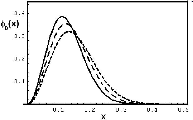
The physics below the factorization scale is non-perturbative in nature, which is described by the hadronic wave functions of mesons. They are not perturbatively calculable, but universal for all the decay processes. Since many of the hadronic and semi-leptonic decays have been measured well in the two B factory experiments, the light wave functions are strictly constrained. Therefore, it is useful to use the same light meson wave functions in our decays determined from the hadronic decays. The uncertainty of the hadronic wave functions will come mainly from the SU(3) breaking effect between the wave function and wave function [7]. In recent years, a lot of studies have been performed for the and decays in the pQCD approach [4]. The parameter has been fixed there using the rich experimental data on the and mesons. In the SU(3) limit, this parameter should be the same in decays. Considering a small SU(3) breaking, the quark momentum fraction here should be a little larger than that of the or quark in the mesons, since the quark is heavier than the or quark. The shape of the distribution amplitude is shown in Fig.1 for , , and . It is easy to see that the larger gives a larger momentum fraction to the quark. We will use in this paper for the decays, which characterize the fact that the quark in meson carries a littler larger momentum fraction than the quark in the meson.
II Results and Discussion
For () meson decays with two light mesons in the final states, the light mesons obtain large momentum of 2.6GeV in the () meson rest frame. All the quarks inside the light mesons are therefore energetic and collinear like. Since the heavy b quark in () meson carries most of the energy of () meson, the light quark in () meson is soft. In the usual emission diagram of () decays, this quark goes to the final state meson without electroweak interaction with other quarks, which is called a spectator quark. Therefore there must be a connecting hard gluon to make it from soft like to collinear like. The hard part of the interaction becomes six quark operator rather than four. The soft dynamics here is included in the meson wave functions. The decay amplitude is infrared safe and can be factorized as the following formalism:
| (1) |
where are the corresponding Wilson coefficients of four quark operators; are the meson wave functions and the factorization scale denotes the largest energy scale of hard process , which is the typical energy scale in pQCD approach. The exponential of function is the so-called Sudakov form factor resulting from the resummation of double logarithms occurred in the QCD loop corrections, which can suppress the contribution from the non-perturbative region.
First we give the numerical results in the pQCD approach for the form factors at maximal recoil. For the form factors, we obtain:
| (2) |
For the form factors, we obtain:
| (3) |
where , (for the and mesons) and GeV, GeV (for the meson). They quantify the SU(3)-symmetry breaking effects in the form factors in the pQCD approach. From these form factors in eq.(2,3), one can notice that the transition form factors are larger than that of due to the SU(3) breaking effect. Usually the same kind of SU(3) breaking effect is also expected between the and transition form factors, but the numbers shown in eq.(2,3) are quite similar. This is due to the fact that the effect of a larger decay constant canceled by a larger parameter of the wave function.
The numerical results of the decays branching ratios and CP asymmetry parameters are displayed in Ref. [4, 7]. Most of the decay channels are measured by B factories; while for charmless decays, only several are measured by the CDF collaboration[9]. The measured branching ratios of and decays are consistent with the theoretical calculations. The calculated branching ratios from the three kinds of methods overlap with each other, considering the still large theoretical and experimental uncertainties.
In table 1, the only measured CP asymmetry in decay prefer our pQCD approach rather than QCDF approach. This is similar with the situation in decays. The direct CP asymmetry is proportional to the sine of the strong phase difference of two decay topologies [6]. The strong phase in our pQCD approach is mainly from the chirally enhanced space-like penguin diagram (annihilation penguin); while in the QCDF approach, the strong phase mainly comes from the virtual charm quark loop diagrams. The different origin of strong phases gives different sign to the direct CP asymmetry imply a fact that the dominant strong phase in the charmless decays should come from the annihilation diagrams. It should be noted that the SCET approach can not predict the direct CP asymmetry of decays directly, since they need more experimental measurements as input. However, it also gives the right CP asymmetry for decay if with the input of experimental CP asymmetries of decays, which means good SU(3) symmetry here [10]. Unlike pQCD approach and QCDF approach, in SCET, the main strong phase responsible for the direct CP asymmetry is from the non-perturbative charming penguins. Although it has the same topology as the annihilation penguin, it may give different mixing induced CP asymmetry for neutral decays [10].
| SCET | QCDF | pQCD | EXP | |
|---|---|---|---|---|
For the branching ratios, the results for QCDF and pQCD approaches are quite similar, which also happens in the decays. The large chiral enhancement factor is adopted in QCDF to give a large penguin contribution here, while in pQCD approach, an additional chirally enhanced penguin annihilation amplitude is included, which gives the same order effect. However, for the channels, the QCDF results are systematically smaller than the pQCD results, which is again happens in the channels, where pQCD results are more favored by B factory experiments. Since there is no more chiral enhancement factor here in the emission type penguin diagram, the QCDF results can not catch up the experiments and the pQCD results with penguin annihilation contributions.
In the decays, again, it is the annihilation penguin diagram gives large transverse polarization contribution to the penguin dominant B decays [11]. For the decays, we also give the polarization fractions in addition to the branching ratios and CP asymmetry parameters [7]. Similar to the decay channels, we also have large transverse polarization fractions for the penguin dominant processes, such as , , decays, whose transverse polarization fraction can reach 40-50%.
III SU(3) breaking effect
| mode () | |||||
|---|---|---|---|---|---|
| 0 | |||||
The SU(3) breaking effect comes mainly from the meson decay constant and distribution amplitude parameter, light meson decay constant and wave function difference, and various decay topology differences. As an example we mainly focus on the decays , , and , as they can be related by SU(3)-symmetry. A question of considerable interest is the amount of SU(3)-breaking in various topologies (diagrams) contributing to these decays. For this purpose, we present in Table 2 the magnitude of the decay amplitudes (squared, in units of GeV2) involving the distinct topologies for the four decays modes. The first two decays in this table are related by U-spin symmetry (likewise the two decays in the lower half). We note that the assumption of U-spin symmetry for the (dominant) tree () and penguin () amplitudes in the emission diagrams is quite good, it is less so in the other topologies, including the contributions from the -exchange diagrams, denoted by for which there are non-zero contributions for the flavor-diagonal states and only. The U-spin breaking is large in the electroweak penguin induced amplitudes , and in the penguin annihilation amplitudes relating the decays and . In the SM, however, the amplitudes are negligibly small.
In and , the branching ratios are very different from each other due to the differing strong and weak phases entering in the tree and penguin amplitudes. However, as shown by He and Gronau [12], the two relevant products of the CKM matrix elements entering in the expressions for the direct CP asymmetries in these decays are equal, and, as stressed by Lipkin [13] subsequently, the final states in these decays are charge conjugates, and the strong interactions being charge-conjugation invariant, the direct CP asymmetry in can be related to the well-measured CP asymmetry in the decay using U-spin symmetry.

Following the suggestions in the literature, we can define the following two parameters:
| (4) | |||||
The standard model predicts and if we assume -spin symmetry. Since we have a detailed dynamical theory to study the SU(3) (and U-spin) symmetry violation, we can check in pQCD approach how good quantitatively this symmetry is in the ratios and . We get and . Thus, we find that these quantities are quite reliably calculable, as anticipated on theoretical grounds. SU(3) breaking and theoretical uncertainties are very small here, because most of the breaking effects and uncertainties are canceled due to the definition of and . On the experimental side, the results for and are: [9]
| (6) |
We conclude that SM is in good agreement with the data, as can also be seen in Fig. 2 where we plot theoretical predictions for vs. and compare them with the current measurements of the same. The measurements of these quantities are rather imprecise at present, a situation which we hope will greatly improve at the LHCb experiment.
IV Summary
Based on the factorization, pQCD approach is infrared safe. Its predictions on the branching ratios and CP asymmetries of the decays are tested well by the B factory experiments. Using those tested parameters from these decays, we predict branching ratios and CP asymmetries of a number of charmless decay channels , and in the perturbative QCD approach. The experimental measurements of the three decay channels are consistent with our numerical results. Especially the measured direct CP asymmetry of agree with our calculations. We also discuss the SU(3) breaking effect in these decays, which is at least around 20-30%. We also show that the He-Gronau-Lipkin sum rule works quite well in the standard model, where the SU(3) breaking effects mainly cancel.
The annihilation penguin diagram is chirally enhanced in the pQCD approach. Its large contribution and strong phase give the right sign for direct CP asymmetry, the large branching ratios for the decays and large transverse polarization fraction for the decays. Its important role is also realized later in the QCDF approach.
Acknowledgements.
We are grateful to the collaborators of this work: A. Ali, G. Kramer, Y. Li, Y.L. Shen, W. Wang and Y.M. Wang. This Work is supported by National Science Foundation of China under Grant No.10735080 and 10625525.References
- [1] M. Wirbel, B. Stech, M. Bauer, Z. Phys. C29, 637 (1985); M. Bauer, B. Stech, M. Wirbel, Z. Phys. C34, 103 (1987).
- [2] A. Ali, G. Kramer, and C. -D. Lü, Phys. Rev. D58, 094009 (1998) [hep-ph/9804363]; Phys. Rev. D59, 014005 (1999) [hep-ph/9805403]; Y. H. Chen, H. Y. Cheng, B. Tseng, and K. C. Yang, Phys. Rev. D60, 094014 (1999) [hep-ph/9903453].
- [3] M. Beneke, G. Buchalla, M. Neubert and C. T. Sachrajda, Phys. Rev. Lett. 83, 1914 (1999) [hep-ph/9905312]; Nucl. Phys. B591, 313 (2000) [hep-ph/0006124].
- [4] Y. Y. Keum, H. n. Li, and A. I. Sanda, Phys. Lett. B504, 6 (2001) [hep-ph/0004004]; Phys. Rev. D63, 054008 (2001) [hep-ph/0004173]; C.D. Lü, K. Ukai and M.Z. Yang, Phys. Rev. D63, 074009 (2001) [hep-ph/0004213]; C.D. Lü and M.Z. Yang, Eur. Phys. J.C23, 275 (2002) [hep-ph/0011238].
- [5] C. W. Bauer, D. Pirjol, I. W. Stewart, Phys. Rev. Lett. 87 (2001) 201806 [hep-ph/0107002]; Phys. Rev. D65, 054022 (2002) [hep-ph/0109045].
- [6] B. H. Hong, C.D. Lü, Sci. China G49, 357-366 (2006) [hep-ph/0505020].
- [7] Y. Li, C.-D. Lu, Z.-J. Xiao, X.-Q. Yu, Phys. Rev. D70, 034009 (2004) [hep-ph/0404028]; X.Q. Yu, Y. Li, C.D. Lu, Phys. Rev. D71, 074026 (2005), Erratum-ibid. D72, 119903 (2005) [hep-ph/0501152]; A. Ali et al., arXiv: hep-ph/0703162.
- [8] H.-n. Li, Prog. Part. & Nucl. Phys. 51, 85 (2003) [hep-ph/0303116], and reference therein.
- [9] M. Morello [CDF Collaboration], FERMILAB-PUB-06-471-E (2006) [hep-ex/0612018].
- [10] A. Williamson and J. Zupan, Phys. Rev. D74, 014003 (2006); Erratum-ibid. D 74, 039901 (2006) [hep-ph/0601214]; W. Wang, Y.-M. Wang, D.S. Yang, C.D. Lu, e-Print: arXiv:0801.3123 [hep-ph]
- [11] H.-n. Li and S. Mishima, Phys. Rev. D71, 054025 (2005); H.-n. Li, Phys. Lett. B622, 63 (2005); H.-W. Huang, et al., Phys. Rev. D73, 014011 (2006), e-Print Archive: hep-ph/0508080; C.H. Chen, e-Print Archive: hep-ph/0601019; Ying Li, Cai-Dian Lu, Phys. Rev. D73, 014204 (2006), e-Print Archive: hep-ph/0508032C.-D. Lü, Y.-l. Shen, J. Zhu, Eur. Phys. J. C41, 311 (2005), hep-ph/0501269; J. Zhu, Y-L. Shen, C.-D. Lu, Phys. Rev. D72, 054015 (2005), e-Print Archive: hep-ph/0504187
- [12] X.G. He, Eur. Phys. J. C9, 443-448 (1999); M. Gronau, Phys. Lett. B492, 297 (2000) hep-ph/0008292].
- [13] H. J. Lipkin, Phys. Lett. B621, 126 (2005) [hep-ph/0503022].