Dimensionally Distributed Learning
Models and AlgorithmThanks: This research was supported in part by the U.S. National Science Foundation under Grants ANI-03-38807 and CNS-06-25637, and by the Office of Naval Research under contract numbers W911NF-07-1-0185 and N0014-07-1-0555.

Haipeng Zheng Affiliation: Department of Electrical Engineering
Princeton University
Princeton, NJ, U.S.A.
Email: haipengz@princeton.edu Sanjeev R. Kulkarni Affiliation: Department of Electrical Engineering
Princeton University
Princeton, NJ, U.S.A.
Email: kulkarni@princeton.edu H. Vincent Poor Affiliation: Department of Electrical Engineering
Princeton University
Princeton, NJ, U.S.A.
Email: poor@princeton.edu

Abstract

This paper introduces a framework for regression with dimensionally distributed data with a fusion center. A cooperative learning algorithm, the iterative conditional expectation algorithm (ICEA), is designed within this framework. The algorithm can effectively discover linear combinations of individual estimators trained by each agent without transferring and storing large amount of data amongst the agents and the fusion center. The convergence of ICEA is explored. Specifically, for a two agent system, each complete round of ICEA is guaranteed to be a non-expansive map on the function space of each agent. The advantages and limitations of ICEA are also discussed for data sets with various distributions and various hidden rules. Moreover, several techniques are also designed to leverage the algorithm to effectively learn more complex hidden rules that are not linearly decomposable.

Keywords: Distributed learning, heterogeneous data, regression, estimation.

I Introduction

Distributed learning is a field that generalizes classical machine learning algorithms. Instead of having full access to all the data and being capable of central computation, in the framework of distributed learning, there are a number of agents that have access to only part of the data. And the agents (perhaps with a fusion center) are capable of exchanging certain types of information among one another. Usually, due to privacy concerns, limited bandwidth and limited power, the content and amount of information shared are restricted. Research in distributed learning seeks effective learning algorithms and theoretical limits within such constraints.

In terms of data structures, two types of distributed learning problems are: homogeneous data and heterogeneous data (or horizontally distributed / instance distributed data and vertically distributed / dimensionally distributed data). In terms of the organization of distributed learning systems, there are also basically two types: systems with a fusion center and systems without a fusion center. In [1], [2] two important types of models, instance distributed learning with and without a fusion center, are discussed and several practical algorithms are provided. The relationship between the information transmitted amongst individual agents and the fusion center and the ensemble learning ability are also discussed. There has also been some research on distributed learning with dimensionally distributed data, such as in [3]. However, the approach in [3] is not cooperative - individual agents first optimize their own estimator, and, given these estimators, the fusion center then constructs an optimal linear combination of them. In this paper, however, we will concentrate on a cooperative training algorithm, in which the fusion center coordinates the individual agents to optimize the ensemble estimator.

It is also worth pointing out the connection between dimensionally distributed learning and boosting for regression, which was first introduced in [5] and developed in many other works such as [6]. The algorithm developed in this paper can be viewed as an $L_{2}$ -regression boosting algorithm with extra constraints on the space from which the weak hypothesis can be selected. This perspective can bring insights of boosting to the problem of distributed regression.

II Description of the Problem

In this paper, we discuss the problem of estimation (or regression) with dimensionally distributed data and a fusion center. The problem is specified as follows.

There are $M$ independent variables (or features) $X_{1},\cdots,X_{M}$ and one dependent variable $Y$ . The complete data set is composed of

\{(x_{i1},x_{i2},\cdots,x_{iM},y_{i})\}_{i=1}^{n}

where $n$ is the number of instances, $x_{ij}\in\mathbb{R}$ is the $i$ -th instance of $X_{j}$ , and $y_{i}\in\mathbb{R}$ is the $i$ -th instance of $Y$ .

We also assume that there exists a hidden deterministic function (or rule, or hypothesis)

\phi:\mathbb{R}^{M}\rightarrow\mathbb{R}

such that

y_{i}=\phi(x_{i1},x_{i2},\cdots,x_{iM})+w_{i}

where $\{w_{i}\}_{i=1}^{n}$ is an independently drawn sample from a zero-mean random variable $W$ that is independent of $X_{1},\cdots,X_{M}$ and $Y$ .

Suppose there are $D$ agents, each of which has only limited access to certain features. Define $F_{j}(j=1,\cdots,D)$ to be the set of features accessible by agent $j$ , and define $F=\cup_{j=1}^{D}F_{j}$ so that $|F|=M$ .

In order to concentrate on the “distributed part” of the problem, we assume that each agent is capable, given enough data, of learning the optimal minimum-mean-square-error (MMSE) estimator based on limited access to the features. More specifically, we assume that agent $j$ can solve the optimization problem (given enough data)

\min_{g_{j}(\{X_{t}\}_{t\in F_{j}})}\mathbb{E}\left[\left(\zeta(\{X_{t}\}_{t\in F})-g_{j}(\{X_{t}\}_{t\in F_{j}})+W\right)^{2}\right]

where $\zeta$ can be any $M$ dimensional function satisfying some regularity conditions. Due to the independence and unbiasedness of the noise, the above optimization problem can be simplified to

\min_{g_{j}(\{X_{t}\}_{t\in F_{j}})}\mathbb{E}\left[\left(\zeta(\{X_{t}\}_{t\in F})-g_{j}(\{X_{t}\}_{t\in F_{j}})\right)^{2}\right]

The solution to the optimization problem above is

g_{j}(x_{F_{j}})=\mathbb{E}[\zeta(X_{F})|X_{F_{j}}=x_{F_{j}}]

where, for simplicity, we use $x_{F_{j}}$ to represent $\{x_{t}\}_{t\in F_{j}}$ ; that is, we assume that each agent is capable of estimating the conditional expectation of a function on $F$ given the several dimensions comprising $F_{j}$ , and based on enough data.

Under this model, one way to deal with the distributed estimation problem is another optimization problem formulated as follows:

\min_{\rho(g_{1},g_{2},\cdots,g_{D})}\mathbb{E}\left[\left(\phi(X_{F})-\rho\left(g_{1}(X_{F_{1}}),\cdots,g_{D}(X_{F_{D}})\right)\right)^{2}\right]

where the functions $g_{i},i=1,\cdots,D$ are fixed and given by the agents. The optimization problem above is intractable in its full generality, and this non-cooperative training approach does not take full advantage of the communication between individual agents and the fusion center (because it uses only one-way agent-to-center communication).

However, if we restrict the function $\rho$ to be of the additive form

\rho(g_{1},g_{2},\cdots,g_{D})=g_{1}+g_{2}+\cdots+g_{D},

and optimize over $g_{j},j=1,\cdots,D$ , i.e. we change this problem into a simplified version

\min_{g_{1},g_{2},\cdots,g_{D}}\mathbb{E}\left[\left(\phi(X_{F})-\left(g_{1}(X_{F_{1}})+\cdots+g_{D}(X_{F_{D}})\right)\right)^{2}\right],

we then change a two-step optimization problem (first individual agents optimize their own estimators, then the fusion center optimizes the ensemble) to a one-step cooperative optimization problem (the agents, with the coordination of the fusion center, optimize the sum of their estimators cooperatively). So we can seek an algorithm through which the agents can cooperatively solve the above problem.

III Communication and Memory Restrictions

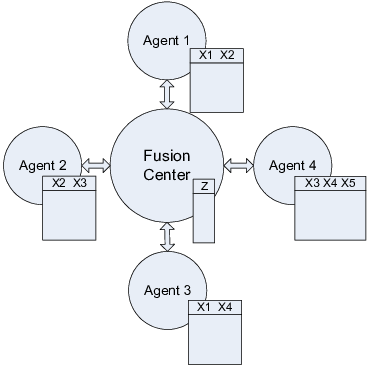
We assume that each agent can store all the data instances of its accessible features, i.e. agent $j$ has access to data $\{x_{it}\}_{i=1}^{n},\forall t\in F_{j}$ . We also assume that the fusion center can store $\{y_{i}\}_{i=1}^{n}$ , which is equivalent to a one-dimensional data set. The agents and fusion center also have an additional one-dimensional memory (which can store all the instances of the dependent variable or one dimension of the features) for computation only, and there is no additional space beyond their own allocation.

We further assume that the fusion center has two-way communication with all the agents. To be more specific, each agent can read and write on the one-dimensional data stored in the fusion center.

Moreover, as noted above, we also require each agent to be capable of finding the ideal MMSE estimator (within a certain function space $\mathcal{F}$ ) based on its accessible data. Fig.1 is an illustration of the structure of a typical dimensionally distributed learning system.

Refer to caption — Figure 1: Structure of a dimensionally distributed learning system for regression.

IV Iterative Conditional Expectation Algorithm

IV-A Basic Idea

Motivated by the backfitting algorithm for additive models in [4], we propose the iterative conditional expectation algorithm (ICEA). The basic idea of this algorithm is very simple: First, agent 1 asks for the value of $\phi(x_{F})$ for all the data instances from the fusion center, makes an estimate based on features in $F_{1}$ and thereby obtains $g_{1}(x_{F_{1}})$ . Of course, $g_{1}(x_{F_{1}})$ cannot fully represent the true function $\phi(x_{F})$ because it lies in a much smaller function space.

Then, agent 1 sends back its estimate for all the data instances to the fusion center, and, the fusion center stores the residual $\phi(x_{F})-g_{1}(x_{F_{1}})$ for all the data instances. Then, agent 2 asks for the value of $\phi(x_{F})-g_{1}(x_{F_{1}})$ from the fusion center, makes an estimate based on features in $F_{2}$ and thereby obtains $g_{2}(x_{F_{2}})$ . This time, $g_{1}(x_{F_{1}})+g_{2}(x_{F_{2}})$ is a better approximation of the true hidden rule $\phi(x_{F})$ .

This process is continued for all agents. When the process eventually returns to agent 1, it then asks the fusion center for the value of $\phi(x_{F})-\sum_{j=1}^{D}g_{j}(x_{F_{j}})$ , thereby obtains $\Delta g_{1}(x_{F_{1}})$ , and stores $(g_{1}+\Delta g_{1})(x_{F_{1}})$ as the updated version of $g_{1}(x_{F_{1}})$ . Then agent 1 sends that value of $\Delta g_{1}(x_{F_{1}})$ for all the instances to the fusion center, and the fusion center obtains the updated version of $\phi(x_{F})-\sum_{j=1}^{D}g_{j}(x_{F_{j}})$ . This continues to agent 2, and so on.

After a few rounds of iteration, the algorithm will converge to a limit (we will show this below, under some further conditions). And the sum of the limit of the functions, i.e.

\sum_{j=1}^{D}g_{j}(x_{F_{j}})

is the best linearly decomposed approximation of $\phi(x_{F})$ in terms of MMSE.

IV-B ICEA in Detail

The following is a more precise description of the above algorithm (in terms of actual data instead of an evolution of ideal functions):

$g_{j}(x_{F_{j}})\leftarrow 0,\forall j\in\{1,\cdots,D\}$ ;

z_{i}\leftarrow y_{i},\forall i\in\{1,\cdots,n\}

;

err_{new}\leftarrow\frac{1}{n}\sum_{i=1}^{n}z_{i}^{2}

;

err_{old}\leftarrow 0

;

while $|err_{old}-err_{new}|>\epsilon$ do for $j$ from $1$ to $D$ do

\Delta g_{j}(x_{F_{j}})\leftarrow

TRAIN

(\{z_{i},\{x_{it}\}_{t\in F_{j}}\}_{i=1}^{n})

;

g_{j}(x_{F_{j}})\leftarrow g_{j}(x_{F_{j}})+\Delta g_{j}(x_{F_{j}})

;

z_{i}\leftarrow z_{i}-\Delta g_{j}(\{x_{it}\}_{t\in F_{j}}),\forall i

;

end

err_{old}\leftarrow err_{new}

;

err_{new}\leftarrow\frac{1}{n}\sum_{i=1}^{n}z_{i}^{2}

;

end function TRAIN(

\{y_{i},\{x_{it}\}_{t\in F}\}_{i=1}^{n}

) return $g(x_{F})$ ;

g(x_{F})=\argmin_{g\in\mathcal{F}}\sum_{i=1}^{n}\left(y_{i}-g(\{x_{it}\}_{t\in F})\right)^{2}

Actually, the

\Delta g_{j}(x_{F_{j}})\leftarrow

TRAIN

(\{z_{i},\{x_{it}\}_{t\in F_{j}}\}_{i=1}^{n})

step, given enough data, is essentially computing

\Delta g_{j}(x_{F_{j}})\leftarrow\frac{\int_{F\setminus F_{j}}\zeta(x_{F})f_{j}(x_{F_{j}})\mathrm{d}\mu}{\int_{F\setminus F_{j}}f_{j}(x_{F_{j}})\mathrm{d}\mu}=\mathbb{E}[\zeta(X_{F})|X_{F_{i}}=x_{F_{i}}]

where the function

\zeta(x_{F})

satisfies

\zeta(\{x_{it}\}_{t\in F})=z_{i}

. This step is handled by individual agents, which we have assumed can be done perfectly. Therefore, if we concentrate on the functional evolution level (instead of on the actual data), the algorithm can be interpreted in terms of iterative conditional expectations:

g_{j}(x_{F_{j}})\leftarrow 0,\forall j\in\{1,\cdots,D\}

;

\zeta(x_{F})\leftarrow\phi(x_{F})

;

err_{new}\leftarrow\mathbb{E}[\zeta^{2}(X_{F})]

;

err_{old}\leftarrow 0

;

while $|err_{old}-err_{new}|>\epsilon$ do for $j$ from $1$ to $D$ do

\Delta g_{j}(x_{F_{j}})\leftarrow\mathbb{E}[\zeta(X_{F})|X_{F_{i}}=x_{F_{i}}]

;

g_{j}(x_{F_{j}})\leftarrow g_{j}(x_{F_{j}})+\Delta g_{j}(x_{F_{j}})

;

\zeta(x_{F})\leftarrow\zeta(x_{F})-\Delta g_{j}(x_{F_{j}})

;

end

err_{old}\leftarrow err_{new}

;

err_{new}\leftarrow\mathbb{E}[\zeta^{2}(X_{F})]

;

endNotice that the training errors are system “biases” caused by the limitation of our “linear decomposition”, and the effects of random error caused by the finite number of training examples. These latter are the same as in classical learning theory and are not factors to be considered as resulting from the “distributed” nature of the problem. Thus, we do not consider them in our discussion. From the point of view of the fusion center, it simply sends its data that represents

\zeta(x_{F})

to an agent, waits for the agent to first update its own estimator

g_{j}(x_{F_{j}})

, and then to send back the difference

\Delta g_{j}(x_{F_{j}})

. The fusion center then updates its data to represent

\zeta(x_{F})-\Delta g_{j}(x_{F_{j}})

, and moves on to the next agent. From the point of view of an individual agent, the task is also straightforward: when agent

j

receives the data describing the latest version of

\zeta(x_{F})

from the fusion center, it finds an optimal estimator

\Delta g_{j}(x_{F_{j}})

\zeta(x_{F})

based on all the data on features in

F_{j}

, uses

\Delta g_{j}(x_{F_{j}})

to update its own estimator

g_{j}(x_{F_{j}})

, and then sends

\Delta g_{j}(x_{F_{j}})

back to the fusion center. In general, the algorithm is simple, and each agent can use its own learning algorithm to determine (approximately) the conditional-mean estimator. It is worth noting that once the estimator is trained, it is distributively allocated throughout the entire system. Thus, when new data comes to the fusion center, it sends features to the corresponding agents and then sums their estimates to form a global estimate.

V Theoretical analysis of ICEA

Intuitively, the above algorithm will repeatedly reduce the power of the residual stored in the fusion center. But does it converge? And, if so, what does it converge to and at what rate? Now let us look at the answers to these questions for some special cases.

The monotonicity of the residual is easy to see. More specifically, the root-mean-square-error (RMSE) of the ensemble estimator is monotonically non-increasing. This is because in ICEA, we repeatedly fix all the individual estimators but one, and optimize only that one and use the new function to replace the old. Thus, the new estimator cannot be worse than the old one, and therefore, the RMSE must be non-increasing.

Moreover, since the RMSE is always non-negative, the RMSE sequence is a monotonically non-increasing, lower bounded sequence, which guarantees the convergence of the algorithm (if we use the change in RMSE as the convergence criterion, which is what we did in the algorithm previously shown). However, there is no guarantee of uniqueness (different initial conditions might lead to different limits), nor of equivalence between the limits and the solution to the optimization problem given in the previous section.

So in the following subsections, we discuss the functional convergence of ICEA under some special cases.

V-A Non-expansive map for two agent case

For the two-dimensional, two-agent case, the algorithm is intended to solve the following optimization problem:

\min_{g_{1},g_{2}}\mathbb{E}\left[\left(\phi(x_{1},x_{2})-g_{1}(x_{1})-g_{2}(x_{2})\right)^{2}\right].

It is straightforward to show that the optimal solution $g_{1,opt}(x_{1})$ and $g_{2,opt}(x_{2})$ should satisfy equations

g_{1}(x_{1})=\mathbb{E}\left[\left(\phi(x_{1},x_{2})-g_{2}(x_{2})\right)|X_{1}=x_{1}\right]

and

g_{2}(x_{2})=\mathbb{E}\left[\left(\phi(x_{1},x_{2})-g_{1}(x_{1})\right)|X_{2}=x_{2}\right]

simultaneously.

On the other hand, if we apply ICEA to the two dimensional distributed learning problem, we will iteratively find the solutions to the equations above. And (hopefully) the solution will converge to the desired $g_{1,opt}(x_{1})$ and $g_{2,opt}(x_{2})$ ; i.e. ICEA enables us to approximate the solution to a difficult optimization problem by solving a sequence of simplified optimization problems iteratively. Of course, rigorously, we need to prove the convergence of this algorithm and the uniqueness of its limit.

Ideally, if we can show that each round of the algorithm is actually a contractive map on a well-defined metric space, it is easy to apply the fixed point theorem to guarantee the uniqueness of the limit.

Unfortunately, we can prove only a weaker conclusion: for the two-agent case, ICEA, after each complete round (i.e. after each agent updates its estimator), is equivalent to a non-expansive map.

First we need to define a suitable measure of distance between two functions $g(x_{F})$ and $h(x_{F})$ :

d\left(g(x_{F}),h(x_{F})\right)=\mathbb{E}\left[(g(X_{F})-h(X_{F}))^{2}\right].

The algorithm performs the following operation to a function $g_{1}(x_{1})$ after each complete round (denote the mapping as $T$ ):

	$\displaystyle T\{g_{1}(X_{1})\}=$
	$\displaystyle\mathbb{E}[\phi(X_{1},X_{2})-\mathbb{E}[\phi(X_{1},X_{2})-g_{1}(X_{1})\|X_{2}]\|X_{1}=x_{1}].$

Therefore, the distance between $T\{g_{1}(x_{1})\}$ and $T\{g_{1}^{*}(x_{1})\}$ is given by

\mathbb{E}\left[\left(\mathbb{E}[\mathbb{E}[g_{1}(X_{1})-g_{1}^{*}(X_{1})|X_{2}]|X_{1}]\right)^{2}\right].

In order to show that $T$ is a non-expansive map, it is equivalent to prove the following inequality:

\mathbb{E}\left[\left(\mathbb{E}[\mathbb{E}[g(X_{1})|X_{2}]|X_{1}]\right)^{2}\right]\leq\mathbb{E}[g^{2}(X_{1})],

where $g(X_{1})=g_{1}(X_{1})-g_{1}^{*}(X_{1})$ .

Define $\mu_{g}=\mathbb{E}[g(X_{1})]$ , and notice two facts:

			$\displaystyle\mathbb{E}\left[\left(\mathbb{E}[\mathbb{E}[g(X_{1})\|X_{2}]\|X_{1}]\right)^{2}\right]-\mu_{g}^{2}$
		$\displaystyle=$	$\displaystyle\mathbb{E}\left[\left(\mathbb{E}[\mathbb{E}[g(X_{1})\|X_{2}]\|X_{1}]-\mu_{g}\right)^{2}\right],$

and

\mathbb{E}\left[g^{2}(X_{1})\right]-\mu_{g}^{2}=\mathbb{E}\left[\left(g(X_{1})-\mu_{g}\right)^{2}\right].

Then, the original inequality is equivalent to the inequality

\mathbb{E}\left[\left(\mathbb{E}[\mathbb{E}[g(X_{1})|X_{2}]|X_{1}]-\mu_{g}\right)^{2}\right]\leq\mathbb{E}\left[\left(g(X_{1})-\mu_{g}\right)^{2}\right].

Then, we have that the left hand side satisfies

$\displaystyle LHS$	$\displaystyle=$	$\displaystyle\mathbb{E}\left[\left(\mathbb{E}[\mathbb{E}[g(X_{1})\|X_{2}]\|X_{1}]-\mathbb{E}[\mathbb{E}[g(X_{1})]\|X_{1}]\right)^{2}\right]$
	$\displaystyle=$	$\displaystyle\mathbb{E}\left[\left(\mathbb{E}[\mathbb{E}[g(X_{1})\|X_{2}]-\mathbb{E}[g(X_{1})]\|X_{1}]\right)^{2}\right]$
	$\displaystyle\leq$	$\displaystyle\mathbb{E}\left[\mathbb{E}[\left(\mathbb{E}[g(X_{1})\|X_{2}]-\mathbb{E}[g(X_{1})]\right)^{2}\|X_{1}]\right]$
	$\displaystyle=$	$\displaystyle\mathbb{E}\left[\left(\mathbb{E}[g(X_{1})\|X_{2}]-\mathbb{E}[g(X_{1})]\right)^{2}\right].$

The inequality step is because of Jensen’s inequality:

\phi[\mathbb{E}(X)]\leq\mathbb{E}[\phi(X)]

when $\phi$ is a (measurable) convex function. Moreover, we also have

\mathbb{E}\left[\left(\mathbb{E}[g(X_{1})|X_{2}]-\mathbb{E}[g(X_{1})]\right)^{2}\right]=\mathrm{Var}\left[\left(\mathbb{E}[g(X_{1})|X_{2}]\right)^{2}\right],

and hence,

LHS\leq\mathrm{Var}\left[\left(\mathbb{E}[g(X_{1})|X_{2}]\right)^{2}\right].

In addition, we have that the right hand side satisfies

RHS=\mathrm{Var}[g(X_{1})],

and an important relationship:

\mathrm{Var}[g(X_{1})]\geq\mathrm{Var}\left[\left(\mathbb{E}[g(X_{1})|X_{2}]\right)^{2}\right]+\mathbb{E}\left[\mathrm{Var}[g(X_{1})|X_{2}]\right].

Therefore,

RHS\geq LHS+\mathbb{E}\left[\mathrm{Var}[g(X_{1})|X_{2}]\right]\geq LHS,

and hence we have proven that $T$ is an non-expansive map. This result can be easily generalized to the two-agent, high dimensional case.

V-B Contractive map for a special case

Non-expansiveness is weaker than contractiveness, and there is no general “fixed-point” theorem. But, under certain conditions, we are able to draw stronger conclusions. For instance, if we restrict the problem to the two-dimensional case, restrict the hidden rule to be a finite order bivariate polynomial, and restrict the distribution of the dependent variables to the two-dimensional joint Gaussian distribution with correlation coefficient $|\rho|<1$ , then ICEA can be shown to be a contractive map.

Moreover, for the two-agent, two-dimension Gaussian case above, we can also measure the speed of convergence by the contractive factor of the contractive map. It can be shown that the factor is $\rho^{4}$ , i.e.¹¹ 1 This is shown in the appendix.

d\left(T(g(X_{1})),T(h(X_{1}))\right)\leq\rho^{4}d\left(g(X_{1}),h(X_{1})\right).

So when the two dimensions are weakly correlated, the convergence can be very fast.

VI Simulation results of ICEA

VI-A Simulation in Terms of Function Evolution

A detailed simulation of the two-agent, two-dimensional, finite-order bivariate-polynomial hidden rule, jointly-Gaussian case is shown below. The hidden rule is

\phi(x_{1},x_{2})=x_{1}x_{2}^{2}+x_{1}^{2}+2,

and $(X_{1},X_{2})$ is jointly Gaussian with zero mean, unit variance and correlation coefficient $\rho=1/2$ .

On initializing $g_{1}(x_{1})$ and $g_{2}(x_{2})$ to be $0$ and applying ICEA to the problem, we get the following results shown in Table I:

Round	$g_{1}(x_{1})$ and $g_{2}(x_{2})$	RMSE
1	$2+.7500x_{1}+x_{1}^{2}+.2500x_{1}^{3}$
	$-.6563x_{2}+.4688x_{2}^{3}$	$1.4941406250$
2	$2+.5508x_{1}+x_{1}^{2}+.1914x_{1}^{3}$
	$-.4907x_{2}+.4761x_{2}^{3}$	$1.2974381447$
3	$2+.4598x_{1}+x_{1}^{2}+.1905x_{1}^{3}$
	$-.4442x_{2}+.4762x_{2}^{3}$	$1.2864467088$
4	$2+.4364x_{1}+x_{1}^{2}+.1905x_{1}^{3}$
	$-.4325x_{2}+.4762x_{2}^{3}$	$1.2857600621$
5	$2+.4305x_{1}+x_{1}^{2}+.1905x_{1}^{3}$
	$-.4295x_{2}+.4762x_{2}^{3}$	$1.2857171467$
6	$2+.4291x_{1}+x_{1}^{2}+.1905x_{1}^{3}$
	$-.4288x_{2}+.4762x_{2}^{3}$	$1.2857144645$
Limit	$2+3/7\penalty\ x_{1}+x_{1}^{2}+4/21\penalty\ x_{1}^{3}$
	$-3/7\penalty\ x_{2}+10/21\penalty\ x_{2}^{3}$	$9/7$

Table I: Step-by-step results of the ICEA.

where the limit function is the unique solution to equations

	$\displaystyle g_{1}(x_{1})$	$\displaystyle=$	$\displaystyle\int_{-\infty}^{\infty}\left(\phi(x_{1},x_{2})-g_{2}(x_{2})\right)f_{X_{2}\|X_{1}}(x_{2}\|x_{1})\mathrm{d}x_{2}$
	$\displaystyle g_{2}(x_{2})$	$\displaystyle=$	$\displaystyle\int_{-\infty}^{\infty}\left(\phi(x_{1},x_{2})-g_{1}(x_{1})\right)f_{X_{1}\|X_{2}}(x_{1}\|x_{2})\mathrm{d}x_{2}.$

The evolution of the functions of Table I is shown in Fig.2 and Fig.3. It is quite clear that there is no visible difference after a few rounds of iterations.

Moreover, the speed of convergence can be measured (approximately) by the surplus RMSE (the difference between the RMSE of the ensemble estimator after the $n$ th iteration and the limit RMSE) as shown in Fig.4. Also notice that in the semi-logarithm plot, the slope $k$ of the line is $-2.79375$ , and $(e^{k})^{1/4}\approx 0.5=\rho$ , which is compatible with our theory in the previous section.

VI-B Simulation on Real Data

Our discussion above always assumes enough training data and perfect individual agents that can find the MMSE estimator. However, to justify the efficacy of ICEA in solving real problems, we test the algorithm with real data, contrary to the functional “simulation” we did in the previous section.

In order to compare the distributed regression to other multi-dimensional regression algorithms, we use three functions used in [7] (originally from [8] and [9]) as the hidden rule to generate our simulation training data sets. The three functions are

•

Friedman-1:

$\phi(\mathbf{x})=10\sin(\pi x_{1}x_{2})+20(x_{3}-1/2)^{2}+10x_{4}+5x_{5}+w$

where $x_{j}\sim U[0,1],j=1\ldots 5$ ;
•

Friedman-2:

$\phi(\mathbf{x})=\left(x_{1}^{2}+\left(x_{2}x_{3}-\frac{1}{x_{2}x_{4}}\right)^{2}\right)^{\frac{1}{2}}+w$

where

$x_{1}\sim U[1,100],$

$x_{2}\sim U[40\pi,560\pi],$

$x_{3},x_{5}\sim U[0,1],$

$x_{4}\sim U[1,11].$
•

Friedman-3:

$\phi(\mathbf{x})=\tan^{-1}\left(\frac{x_{2}x_{3}-\frac{1}{x_{2}x_{4}}}{x_{1}}\right)+w$

where the distribution of the features are the same as that of Friedman-2.

All the feature variables are independent, and before running the algorithm, the outcomes are normalized to the range $[0,1]$ . Also, to highlight the effect of distributiveness of the system, the independent white noise $w$ is set to zero in our simulation. Also, it is worth pointing out that in Friedman-2 and Friedman-3, feature $X_{5}$ is irrelevant, and is set up as a test of the algorithm’s resistance to irrelevant features.

Moreover, we did the experiments on three different types of distributed regression systems:

•

System-1: five 1-dimensional agents

$\{X_{1}\},\{X_{2}\},\{X_{3}\},\{X_{4}\},\{X_{5}\}$
•

System-2: three 2-dimensional agents

$\{X_{1},X_{2}\},\{X_{2},X_{3}\},\{X_{4},X_{5}\}$
•

System-3: two 5-dimensional agents

$\{X_{1},X_{2},X_{3}\},\{X_{2},X_{4},X_{5}\}$

In all these cases, all the features are fully covered by the union of the features observable by individual agents.

We use a regression tree - a commonly used “weak learner” in the boosting algorithms - as our learning algorithm for the individual agents. Notice that $L_{2}$ -regression boosting (introduced in [10]) is equivalent to a one-agent system, in which all the dimensions are accessible by the agent. In this sense, $L_{2}$ -regression boosting is the “limit algorithm” of the ICEA for distributed systems. So it is natural to compare the performance of distributed system to $L_{2}$ -regression boosting. Also, to compare the cooperative algorithm ICEA to non-cooperative algorithm (like the algorithms in [3]), we also ran the data on a hierarchical algorithm. The individual agents are identical to those of ICEA, and the fusion center can further train an estimator using $L_{2}$ -regression boosting, taking the output of the agents as the features.

Running three different types of algorithms on three different data sets, with 2000 training data points and 4000 test data points, the mean squared errors are shown in Table II, and the detailed plot of training/test error after each round of $L_{2}$ -regression boosting and ICEA with three different distributed systems running on data set Friedman-2 are shown in Fig. 5.

Data Set	System	ICEA	Hierarchical	$L_{2}$ Boosting
	1	$.0050$	$.024$
Friedman-1	2	$.0014$	$.061$	.0051
	3	$.0039$	$.036$
	1	$.010$	$.075$
Friedman-2	2	$.0012$	$.079$	.00066
	3	$.00088$	$.13$
	1	$.0082$	$.35$
Friedman-3	2	$.0062$	$.23$	.0034
	3	$.0035$	$.31$

Table II: Test error (mean squared error) of

L_{2}

-regression boosting, ICEA and hierarchical on data sets Friedman-1,-2 and -3.

As expected, $L_{2}$ -regression boosting performs best for most of the cases, except for Friedman-1, the hidden hypothesis of which is basically additive. Because System-2 is not so complicated yet is complex enough to fully capture the model, the ICEA algorithm running on System-2 performs best. However, for Friedman-2 and Friedman-3, where the hidden models are no longer additive, $L_{2}$ -regression boosting, with full access to all the dimensions, outperforms other algorithms. And for ICEA, the performance is better when the individual agents have access to more dimensions, capable of describing more complex coupling among the features. The hierarchical algorithm works (thought not so well) for additive models, yet the algorithm performs poorly for data sets with complicated functions where there is strong coupling among the features. Since the estimators used for individual agents in ICEA and the hierarchical algorithm are identical (regression trees), the performance difference can be attributed to the benefit of applying cooperative training in ICEA.

VII Problems of ICEA and Possible Improvements

VII-A Limitations of ICEA

Of course, since we restrict our approximation of $\phi(x_{F})$ to the sum $\sum_{j=1}^{D}g_{j}(x_{F_{j}})$ , we lose richness of the ensemble estimator. For instance, for the function $\phi(x_{1},x_{2})=x_{1}x_{2}$ with $X_{1},X_{2}$ being independent standard Gaussian variables, if agent 1 has access only to dimension 1, and agent 2 has access only to dimension 2, then the linear model estimator is simply $0$ , which means nothing can be learned. So restricting to a linear form can lead to some serious problems. However, there are several ways to solve this problem and greatly expand the efficacy of ICEA.

First, we can linearize the function $\phi(x_{F})$ . For instance, in the example above, if we take the logarithm of the function $\phi(x_{1},x_{2})=x_{1}x_{2}$ , then we get $\log(\phi(x_{1},x_{2}))=\log(x_{1})+\log(x_{2})$ . In this case, we can use the linear additive model to accurately depict the ensemble function. Therefore, with a proper non-linear transformation, we can greatly expand the scope of problems that can be optimally solved by our linear additive model.

Second, we can project the function $\phi(x_{F})$ on more linear combinations of the features of the agents. For instance, in the above problem, if we have two other agents that have access to data $x_{1}+x_{2}$ and $x_{1}-x_{2}$ , then the model can also be accurately learned by these two agents. In practice, because there is significant redundancy amongst the data of the agents, we don’t need to intentionally calculate these linear combinations (which requires more communication resources). Instead, we simply take advantage of the redundancies contained in the data, which is often considered to be a hazard in some learning algorithms.

VII-B Developing More Intelligent Algorithms

Boosting for regression sheds light on the design of algorithms more “intelligent” than ICEA, which simply refits the residual on each agent one after another. ICEA can be improved in more ways than one, in terms of increasing speed of convergence, finding a natural stopping rule to avoid over-training and to reduce generalization error. Several rudimentary experiments have shown that, instead of iteratively refitting the residual one agent after another to reduce merely the training error, we are better off if we choose among the agents more intelligently, and take both the training error on the residual and the complexity of the model into consideration. For instance, a greedy algorithm that always chooses the agent that provides the minimum training error can greatly increase the speed of convergence, and an algorithm using the size of the decision tree as a penalty term can effectively reduce overtraining. It is worthwhile to explore more subtle rules of selecting estimators from agents and more delicate ways to combine them. ICEA is perhaps the most intuitive algorithm, but far from the optimal one.

VIII Conclusions

By restricting the ensemble estimator to an additive form (linear combination of individual estimators), we have developed an iterative algorithm (ICEA) that is guaranteed, under certain conditions, to converges to a unique limit function (or rule, or hypothesis). This limit is an approximation of the true function, and, with the help of some additional features (linearization, redundant data), the approximation can be quite accurate. ICEA also works quite well with real data, with enough training points and properly selected individual estimators. By sending only the predictions and withhold the data, ICEA also preserves the privacy of data of individual agents. There are still many aspects of the algorithm that can be changed to improve the performance of distributed regression, and these are of interest for further investigation.

IX Appendix

Lemma 1 Suppose $g$ is a polynomial of order $M$ ,

g(x)=\sum_{n=0}^{M}a_{n}x^{n},

and $g^{\prime}(x)$ is given by

g^{\prime}(x)=\int_{-\infty}^{\infty}\left(\int_{-\infty}^{\infty}g(x)f_{X|Y}(x|y)\mathrm{d}x\right)f_{Y|X}(y|x)\mathrm{d}y.

Then, with the additional assumption that

\int_{-\infty}^{\infty}g(x)f_{X}(x)\mathrm{d}x=0.

we have inequality

\frac{\int_{-\infty}^{\infty}g^{\prime 2}(x)f_{X}(x)\mathrm{d}x}{\int_{-\infty}^{\infty}g^{2}(x)f_{X}(x)\mathrm{d}x}\leq\rho^{4},

where $f_{X|Y}$ , $f_{Y|X}$ , and $f_{X}$ are all probability densities derived from the joint Gaussian distribution of zero mean, unit variance and correlation $\rho$ .

Proof: The conditional distribution of $X$ given $Y$ and the distribution of $Y$ given $X$ are

X|Y\sim N(\rho y,1-\rho^{2}),

Y|X\sim N(\rho x,1-\rho^{2}).

Therefore, we have

g^{\prime}(x)=\sum_{n=0}^{M}a_{n}\frac{\mathrm{d}^{n}}{\mathrm{d}t^{n}}\exp{\{\rho^{2}xt+\frac{(1-\rho^{4})t^{2}}{2}\}}\arrowvert_{t=0}.

Notice that the exponential term, with proper manipulation, can be expressed in the form of the sum of Hermitian polynomials. Thus, on defining

X=\frac{\rho^{2}}{i\sqrt{2(1-\rho^{2})}}x,s=i\sqrt{\frac{1-\rho^{4}}{2}}t,

we have

\exp{\{\rho^{2}xt+\frac{1-\rho^{4}}{2}t^{2}\}}=e^{2Xs-s^{2}}=\sum_{k=0}^{\infty}H_{k}(X)\frac{s^{k}}{k!}.

Then the expression of $g^{\prime}(x)$ can be rewritten as

	$\displaystyle g^{\prime}(x)$	$\displaystyle=$	$\displaystyle\sum_{n=0}^{M}a_{n}\frac{\mathrm{d}^{n}}{\mathrm{d}t^{n}}\left(\sum_{k=0}^{\infty}H_{k}(X)\frac{s^{k}}{k!}\right)\|_{s=0}$
		$\displaystyle=$	$\displaystyle\sum_{n=0}^{M}a_{n}H_{n}(X)\left(i\sqrt{\frac{1-\rho^{4}}{2}}\right)^{n}.$

Therefore, we have a closed-form expression for $g^{\prime}(x)$ , which is also an $M^{\mathrm{th}}$ -order polynomial:

	$\displaystyle g^{\prime}(x)$	$\displaystyle=$	$\displaystyle\sum_{n=0}^{M}a_{n}H_{n}\left(\frac{\rho^{2}}{i\sqrt{2(1-\rho^{4})}}x\right)\left(i\sqrt{\frac{1-\rho^{4}}{2}}\right)^{n}$
		$\displaystyle=$	$\displaystyle\sum_{n=0}^{M}a_{n}\sum_{k=0}^{\left[\frac{n}{2}\right]}\frac{n!}{k!(n-2k)!}\left(\frac{1-\rho^{4}}{2}\right)^{k}(\rho^{2}x)^{n-2k}.$

By computation, we can derive

\int_{-\infty}^{\infty}g^{2}(x)f_{X}(x)\mathrm{d}x=\sum_{n=0}^{M}n!\left(\sum_{k=0}^{\left[\frac{M-n}{2}\right]}a_{n+2k}\frac{(n+2k)!}{2^{k}n!k!}\right)^{2},

and

\int_{-\infty}^{\infty}g^{\prime 2}(x)f_{X}(x)\mathrm{d}x=\sum_{n=0}^{M}(\rho^{4})^{n}n!\left(\sum_{k=0}^{\left[\frac{M-n}{2}\right]}a_{n+2k}\frac{(n+2k)!}{2^{k}n!k!}\right)^{2}.

Moreover, since $g$ is of zero mean,

\sum_{k=0}^{\left[\frac{M}{2}\right]}a_{2k}\frac{(2k)!}{2^{k}k!}=0.

Therefore,

			$\displaystyle\frac{\int_{-\infty}^{\infty}g^{\prime 2}(x)f_{X}(x)\mathrm{d}x}{\int_{-\infty}^{\infty}g^{2}(x)f_{X}(x)\mathrm{d}x}$
		$\displaystyle=$	$\displaystyle\frac{\sum_{n=1}^{M}(\rho^{4})^{n}n!\left(\sum_{k=0}^{\left[\frac{M-n}{2}\right]}a_{n+2k}\frac{(n+2k)!}{2^{k}n!k!}\right)^{2}}{\sum_{n=1}^{M}n!\left(\sum_{k=0}^{\left[\frac{M-n}{2}\right]}a_{n+2k}\frac{(n+2k)!}{2^{k}n!k!}\right)^{2}}$
		$\displaystyle\leq$	$\displaystyle\frac{\sum_{n=1}^{M}\rho^{4}n!\left(\sum_{k=0}^{\left[\frac{M-n}{2}\right]}a_{n+2k}\frac{(n+2k)!}{2^{k}n!k!}\right)^{2}}{\sum_{n=1}^{M}n!\left(\sum_{k=0}^{\left[\frac{M-n}{2}\right]}a_{n+2k}\frac{(n+2k)!}{2^{k}n!k!}\right)^{2}}$
		$\displaystyle=$	$\displaystyle\rho^{4}.\oblong$

If the hidden rule $\phi(x_{1},x_{2})$ is restricted to a bivariate polynomial with finite order $M$ and zero mean, and $g_{1}(x_{1}),g_{2}(x_{2})$ are both initialized as 0, then after each iteration, $g_{1}(x_{1})$ and $g_{2}(x_{2})$ will remain in the space of zero-mean polynomials of finite order $M$ . If we define the distance between two polynomials $g_{1}(x)$ and $g_{2}(x)$ as $\int_{-\infty}^{\infty}\left(g_{1}(x)-g_{2}(x)\right)^{2}f_{X}(x)\mathrm{d}x,$ then, according to Lemma 1, the map $T$ that convert $g(x)$ to $g^{\prime}(x)$ is a contractive map. Because under our definition of the distance, the space of zero-mean polynomials is complete, we can apply the contractive mapping theorem to guarantee the functional convergence of ICEA for the two-agent, two-dimensional, joint-Gaussian, finite-order-polynomial case. Moreover, also by the lemma, the “contractive factor” of the map is $\rho^{4}$ . As for the hidden rule with non-zero mean, the bias is also addressed by the constant term of the first agent, which will remain the same in the following iterations and hence has no influence on the convergence.

References

[1] J.B. Predd, S.R. Kulkarni and H.V. Poor, “Distributed learning in wireless sensor networks,” IEEE Signal Processing Magazine, vol. 23, pp. 56–69, 2006.
[2] J.B. Predd, Topics in Distributed Inference, Ph.D. thesis, Department of Electrical Engineering, Princeton University, Princeton, NJ, 2006.
[3] S. Merugu and J. Ghosh, “A distributed learning framework for heterogeneous data sources,” Proceeding of the 11th ACM SIGKDD International Conference on Knowledge Discovery in Data Mining, vol. 1, no. 1, pp. 208–217, Chicago, IL, 2005.
[4] T. Hastie, R. Tibshirani and J. Friedman, The Elements of Statistical Learning, Springer, New York, 2001.
[5] J. Friedman, “Greedy function approximation: A gradient boosting machine, ” Annals of Statistics, vol. 23, pp. 1189-1232, 2001.
[6] P. Bühlmann, “Boosting methods: Why they can be useful for high-dimensional data,” Proceedings of the 3rd International Workshop on Distributed Statistical Computing, Vienna, Austria, 2003.
[7] G. Ridgeway, D. Madigan and T. Richardson, “Boosting methodology for regression problems,” Proceedings of Artificial Intelligence and Statistics ’99, pp. 152-161, Fort Lauderdale, FL, 1999.
[8] J. Friedman, E. Grosse and W. Stuetzle, “Multidimensional additive spline approximation,” SIAM Journal on Scientific and Statistical Computing, vol. 4, no. 2, pp. 291-301, 1983.
[9] J. Friedman, “Multidimensional adaptive regression splines,” Annals of Statistics, vol. 19, pp. 1-82, 1991.
[10] P. Bühlmann and B. Yu, “Boosting with the $L_{2}$ -loss: Regression and classification,” Journal of the American Statistical Association, vol. 98, no. 462, pp. 324–339, 2003.

Dimensionally Distributed Learning Models and AlgorithmThanks: This research was supported in part by the U.S. National Science Foundation under Grants ANI-03-38807 and CNS-06-25637, and by the Office of Naval Research under contract numbers W911NF-07-1-0185 and N0014-07-1-0555.

Abstract

I Introduction

II Description of the Problem

III Communication and Memory Restrictions

IV Iterative Conditional Expectation Algorithm

IV-A Basic Idea

IV-B ICEA in Detail

V Theoretical analysis of ICEA

V-A Non-expansive map for two agent case

V-B Contractive map for a special case

VI Simulation results of ICEA

VI-A Simulation in Terms of Function Evolution

VI-B Simulation on Real Data

VII Problems of ICEA and Possible Improvements

VII-A Limitations of ICEA

VII-B Developing More Intelligent Algorithms

VIII Conclusions

IX Appendix

References

Dimensionally Distributed Learning
Models and AlgorithmThanks: This research was supported in part by the U.S. National Science Foundation under Grants ANI-03-38807 and CNS-06-25637, and by the Office of Naval Research under contract numbers W911NF-07-1-0185 and N0014-07-1-0555.