{preliminary}

DescribeX: A Framework for Exploring and Querying XML Web Collections

Flavio Rizzolo

Abstract

The nature of semistructured data in web collections is evolving. Even when XML web documents are valid with regard to a schema, the actual structure of such documents exhibits significant variations across collections for several reasons: an XML schema may be very lax (e.g., to accommodate the flexibility needed to represent collections of documents in RSS¹¹ 1 http://www.rss-specifications.com/ feeds), a schema may be large and different subsets used for different documents (e.g., this is common in industry standards like UBL²² 2 http://oasis-open.org/committees/ubl/), or open content models may allow arbitrary schemas to be mixed (e.g., RSS extensions like those used for podcasting). A schema alone may not provide sufficient information for many data management tasks that require knowledge of the actual structure of the collection.

Web applications (such as processing RSS feeds or web service messages) rely on XPath-based data manipulation tools. Web developers need to use XPath queries effectively on increasingly larger web collections containing hundreds of thousands of XML documents. Even when tasks only need to deal with a single document at a time, developers benefit from understanding the behaviour of XPath expressions across multiple documents (e.g., what will a query return when run over the thousands of hourly feeds collected during the last few months?). Dealing with the (highly variable) structure of such web collections poses additional challenges.

This thesis introduces DescribeX, a powerful framework that is capable of describing arbitrarily complex XML summaries of web collections, providing support for more efficient evaluation of XPath workloads. DescribeX permits the declarative description of document structure using all axes and language constructs in XPath, and generalizes many of the XML indexing and summarization approaches in the literature. DescribeX supports the construction of heterogenous summaries where different document elements sharing a common structure can be declaratively defined and refined by means of path regular expressions on axes, or axis path regular expression (AxPREs). DescribeX can significantly help in the understanding of both the structure of complex, heterogeneous XML collections and the behaviour of XPath queries evaluated on them.

Experimental results demonstrate the scalability of DescribeX summary refinements and stabilizations (the key enablers for tailoring summaries) with multi-gigabyte web collections. A comparative study suggests that using a DescribeX summary created from a given workload can produce query evaluation times orders of magnitude better than using existing summaries. DescribeX’s light-weight approach of combining summaries with a file-at-a-time XPath processor can be a very competitive alternative, in terms of performance, to conventional fully-fledged XML query engines that provide DB-like functionality such as security, transaction processing, and native storage.

To my parents,

Ofelia and Juan Carlos

Acknowledgements

This thesis is the culmination of my graduate studies at the University of Toronto. It goes without saying that no scientific work can be carried out in isolation, and this one is no exception. I would like to thank here all the people who helped me along the way.

First and foremost, I wish to express my utmost gratitude to Alberto Mendelzon and Renée Miller, both of whom have been a source of inspiration for many years. They were also the Alpha and the Omega of my graduate studies: Alberto was my advisor during my master’s and the early years of my PhD, and also the first one to suggest the idea of a framework upon which this thesis is based; Renee supervised the final stages of the work and made sure that all the pieces fitted together. Both provided me with support and guidance well beyond the call of duty. They really made this work possible.

Special thanks go to José María Turull Torres and Alejandro Vaisman, great friends and mentors. José María introduced me to the fascinating world of scientific research and encouraged me to pursue graduate studies. I could never thank him enough for his guidance in the first steps of my research career. Alejandro’s encouragement and insight were always invaluable, especially during the most difficult times of my PhD (he was my thesis advisor in disguise for many years). I consider them my academic role models for their integrity and professionalism.

I would like to thank the members of my PhD committee, Kelly Lyons, Thodoros Topaloglou, and John Mylopoulos, for their insightful comments, and Frank Tompa for his thorough external appraisal. I also wish to acknowledge the contribution of Mariano Consens, who helped in the development of some core ideas of this thesis.

I am deeply indebted to the administrative staff of the Department of Computer Science for assisting me in so many different ways. Joan Allen and Linda Chow deserve a special mention.

I am also grateful to the Department of Computer Science, the Natural Sciences and Engineering Research Council of Canada, and the IBM Center for Advanced Studies for their generous financial support at different times over my years of graduate studies.

I want to express my heartfelt appreciation to my many friends in Toronto and abroad, especially to my best officemate, Attila, and to my musical buddies, Diego, Danny, Fabricio, Gustavo and Santi; and in general to all those that had to put up with me for years: Adriana, Adrian, Alberto, Alejandra, Christian, Ceci, Carlos, Clau, Fernanda, Fernando, Frank, Jime, Lily, Lore, Mara, Pachi, Patricia, Rosana, Sebastian and Vivi. Each in their one way made my life more meaningful and enjoyable.

I am also in debt with my parents, Ofelia and Juan Carlos, for helping me to become who I am. I owe them much, and regret that I missed my best opportunities to repay. I dedicate this thesis to them.

Above all, I have to thank a thousand times to my wife, Mariana, the person without whom this thesis could have never been written. Her support and unconditional love are beyond words. It is hard to know who I would be without her; I hope never to have the occasion to find out.

Chapter 1 Introduction

XML is widely used as a common format for web accessible data (e.g., hypertext collections like Wikipedia) as well as for data exchanged among web applications (e.g., blogs, news feeds, podcasts, web services messaging). This data is often referred to as semistructured for the lack of a clear separation between data and metadata it represents: tags (metadata) and content (data) are mixed together in the same XML file.

The vast majority of software tools used for managing XML rely on XPath [W3C07] as the core dialect for XML querying. Hence, web developers use XPath queries for many of the tasks involved in the processing of XML collections. Such collections are normally handled one document at a time, whether the document is an individual RSS¹¹ 1 http://www.rss-specifications.com/ file (used by content distributors to deliver to subscribers frequently updated content over the Web), a single SOAP²² 2 http://www.w3.org/TR/soap/ message, or a Wikipedia article in XHTML.

Even when XML collections have a schema (which can be either a DTD³³ 3 http://www.w3.org/TR/REC-xml or an XML Schema⁴⁴ 4 http://www.w3.org/TR/xmlschema-1/), the actual structure present in each document may exhibit significant variations for several reasons. First, schemas can be very lax. One reason for this is the extensive use of the <xsd:choice> construct in XML schemas, which allows optional elements to occur any number of times, including zero. Such a construct is very common in RSS for instance. Second, a schema can be very large and only subsets are actually used in a given instance. This is the situation with several industry specific standards that contain hundreds of elements, such as UBL⁵⁵ 5 http://oasis-open.org/committees/ubl/ or HR-XML⁶⁶ 6 http://hr-xml.org . UBL and HR-XML are standard libraries of XML schemas that support a variety of business processes. UBL is designed to handle supply chain transactions such as purchase orders, shipping notices, and invoices, whereas HR-XML contains schemas for human resource management such as resumes, payroll information, and benefits enrollment. Finally, a schema can be extended by using the <xsd:any> XML Schema construct, which allows arbitrary content from other schemas to appear under a given element. Such a construct enables different user communities to pick and choose how to combine schemas. Consequently, it provides great flexibility, but makes it harder to determine the structure of the documents that actually appear in a given collection. Examples of the <xsd:any> extensions can be found in a wide variety of industry standards, including RSS, UBL and HR-XML. For instance, the UBL standard permits a contractor to represent invoice documents that include HR-XML TimeCard elements for the contractor employee’s time and expenses. The actual structure of invoice collections will vary significantly across contractors and customers. If an enclosing messaging schema is used, even the UBL and HR-XML fragments in the document can be replaced by other invoicing and time billing schemas. In these scenarios, schemas alone are insufficient for understanding the structure (metadata) of the documents in the collection for either writing or optimizing XPath evaluation.

A developer working with this type of collection faces several challenges. She must learn enough about the structure present in the XML collection to be able to write meaningful XPath queries. She must also develop an understanding of how the XPath expressions behave across different documents in the collection. Even when a task deals with a single document at a time, the developer needs to extrapolate the behaviour of queries over a single document across the entire collection over which the task may be repeatedly applied. In this context, understanding the actual metadata of a web collection can be a significant barrier, even for collections validated against a schema.

Refer to caption — Figure 1.1: Wikipedia document graph (a) and its incoming path summary (b)

XML structural summaries are graphs representing relationships between sets of XML elements (i.e., extents). Unlike schemas, which prescribe what may and may not occur in an instance, summaries provide a description of the metadata that is actually present in a given collection. Figure 1.1 (a) shows the instance graph of a Wikipedia sample document in which nodes correspond to XML elements in the document. Nodes have an id and are labeled with their element names. The structure in Figure 1.1 (b) is a typical summary that groups together instance nodes with the same incoming label paths. In such a summary, two nodes that have the same incoming label path from the root belong to the same extent (sets located below each summary node in the figure). For instance, wikilink elements appear at the end of three different label paths – article.section.wikilink (in blue), article.section.section.wikilink (in red), and article.par.wikilink (in green). Consequently, there are three different wikilink nodes in the summary, one with extent $\{3,16\}$ , another with extent $\{6,11\}$ , and a last one with extent $\{18\}$ . Extents can also be viewed as mappings between instance (document) nodes and summary nodes – represented in the figure by dashed arrows linking wikilink nodes in the document graph (left) and wikilink extents in the incoming path summary (right). An edge $(s_{i},s_{j})$ in the summary means that at least one node in the extent of $s_{i}$ is the parent of at least one node in the extent of $s_{j}$ . For instance, an edge from node $s_{7}$ to $s_{9}$ means that some figure elements within par have caption elements, but not necessarily all of them have (for this document only node 12 has a caption element).

Describing metadata in semistructured collections was a major motivation in one of the earliest summary proposals in the literature [NUWC97, GW97]. Since then, research on summaries has focused on query processing, making summaries one of the most studied techniques for query evaluation and indexing in XML (and other semistructured) data models [MS99, KBNK02, KSBG02, QLO03, BCF+05], as well as for providing statistics useful in XML query estimation and optimization [PG06b].

Most of the existing summary proposals define all extents using the same criteria, hence creating homogeneous summaries. These summaries are based on common element paths (in some cases limited to length $k$ ), including incoming paths (e.g., representative objects [NUWC97], dataguides [GW97], 1-index [MS99], ToXin [RM01], A(k)-index [KSBG02]), both incoming and outgoing paths (e.g., F&B-Index [KBNK02]), or sequences of outgoing paths (e.g., Skeleton [BCF+05]). The few examples of heterogeneous summaries that can adapt/change their structure based on a dynamic query workload (e.g., APEX [CMS02], D(k)-index [QLO03], XSKETCH [PG06b]) compute the extents from statistics and workload information.

However, none of these proposals can help us to find elements based on order and cardinality criteria. Consider again the instance in Figure 1.1. What are the par elements that contain two figures? How many section elements contain a figure with caption next to a table? How many of those contain more than one figure? These are questions that cannot be answered with any of the summaries mentioned above.

Moreover, since these proposals are algorithmically defined, it is hard to determine how they can be used together for processing today’s increasingly heterogeneous and large web collections effectively. Specifically, the summary information is not defined declaratively, limiting the ease with which these summaries can be used within standard data management tasks.

In this thesis, we propose a novel approach for flexibly summarizing the structure of metadata actually present in an XML collection. We introduce DescribeX, a framework that supports constructing heterogenous summaries, where each set in the partition can be defined by means of path regular expressions on axes, or axis path regular expression (AxPRE, for short). AxPREs provide the flexibility necessary for declaratively defining complex mappings between instance nodes and summary nodes capable of expressing order and cardinality, among other properties. Each AxPRE can be specified by the user or obtained from any expression in the complete XPath language (all the axes, document order, use of parenthesis, etc.). Given an arbitrary XPath expression posed by the user, DescribeX can create a partition defined by an AxPRE that captures exactly the structural commonality expressed by a query. AxPRE summaries have a unique capability that makes them suitable for describing the structure of XML collections: they are the first summaries capable of declaratively defining and refining the summary extents using a powerful language. In addition, DescribeX summaries express relationships between instance nodes that go beyond the traditional parent-child (e.g., next sibling, following, preceding, etc.). Last but not least, DescribeX captures most summary proposals in the literature by providing a declarative definition for them for the first time.

This thesis argues that DescribeX can significantly help not only in the understanding of the structure of large collections of XML documents, but also in the evaluation of XPath queries posed on them. In fact, DescribeX summaries can also be used to significantly speed up (and scale up) XPath evaluation over existing file-at-a-time tools, enabling fast exploration of the results of XPath workloads on large collections. The experimental results demonstrate that using a summary created from a given workload can produce query evaluation times that are two orders of magnitude better than using existing summaries (in particular, summaries on incoming paths like 1-index [MS99], APEX [CMS02], A(k)-index [KSBG02], and D(k)-index [QLO03]). The experiments also validate that DescribeX summaries allow file-at-a-time XPath processors to be a competitive light-weight alternative (in terms of performance) to conventional DB-like XML query engines supporting additional functionality such as security, transaction processing, and native storage.

DescribeX also has applications to helping a user write and understand XPath queries on large XML collections. Several software tools have been developed to help XPath users debug query expressions (e.g., Oxygen XML Editor⁷⁷ 7 http://www.oxygenxml.com/, Altova XMLSpy⁸⁸ 8 http://www.altova.com/, etc.) A recent research project includes a tool, XPlainer-Eclipse [CLR07], that provides visual explanations of XPath expressions. An explanation returns precisely the nodes in a document that contribute to the answer, a useful debugging technique. However, the main limitation of traditional XPath debugging tools in the context of large XML collections is that they provide debugging mechanisms only for a single document. Understanding queries over collections containing thousands of documents (or even 650,000 documents, like in the Wikipedia XML Corpus [DG06]) using these tools can be an impractical and very time-consuming task. DescribeX provides an important foundation on which such a large-scale XML collection understanding tool could be built, as evidenced by the DescribeX-Eclipse tool presented in Appendix B.

1.1 Major contributions

This thesis identifies the growing need for describing the structure of web collections (encoded in XML) using mechanisms that go beyond providing one or more schemas. We propose the use of highly customizable summaries that represent the actual structure of metadata labels as used in a given collection. The following are the major contributions of this thesis.

1.1.1 AxPRE summaries

AxPRE summaries rely on the novel concept of a summary descriptor (SD). Traditional summaries consist of a labeled graph that describes the label paths in the instance (which we call an SD graph) together with an extent relation between summary nodes and sets of instance nodes. An SD incorporates three key original features:

A description of the neighborhood of a node expressed by path regular expressions on axes (i.e., binary relations between nodes), AxPREs for short (Chapter 3).

AxPREs are evaluated on an axis graph, which is an abstract representation of the XPath data model [W3C07] extended with edges that represent XPath axis binary relations. Edges are labeled by axis names and nodes are labeled by element or attribute names (including namespaces), or by new labels defined using XPath.

Given an axis graph $\mathcal{A}$ , an AxPRE $\alpha$ applied to a node $v$ in $\mathcal{A}$ returns an AxPRE neighbourhood of $v$ which provides a description of the subgraph local to $v$ that satisfies $\alpha$ . The AxPRE neighbourhood of $v$ by $\alpha$ is computed by intersecting the automaton constructed from the axis graph and the automaton accepting the language generated by the AxPRE and all its prefixes.

The AxPRE neighbourhood of a node $v$ is used to determine to which equivalence class $v$ belongs. That is, if two nodes in $\mathcal{A}$ have similar AxPRE neighbourhoods (i.e. they cannot be distinguished by $\alpha$ ), they belong to the same equivalence class. This way, an AxPRE can be used to define a partition of nodes in $\mathcal{A}$ in which each set is the extent of a node $s$ in the SD. The notion of similarity we use is the familiar notion of bisimulation [PT87].

The use of AxPREs neighbourhoods supports the definition of summaries that go beyond the traditional parent and child hierarchical relationships covered by the abundant literature on summaries [GW97, MS99, KBNK02, KSBG02, PG02, QLO03, BCF+05, PG06b]. In particular, AxPREs can describe heterogeneous SDs, i.e., SDs described by multiple AxPREs.

An extent expression (EE) capable of computing precisely the set of elements in the extent of a given SD node (Chapter 5.1).

Since an AxPRE $\alpha$ is used to compute by bisimulation an entire partition, we can say that all sets in the partition share the same AxPRE $\alpha$ . Thus, AxPREs cannot be used to uniquely identify each equivalence class (extent) in such partition (unless the partition contains only one set).

For a large class of neighbourhoods, it is possible to precisely characterize the extent of an SD node $s$ with a new type of expression we call extent expression (EE, for short). The EE $e_{s}$ of $s$ with AxPRE $\alpha$ is generated from the bisimilarity contraction of the $\alpha$ neighbourhoods of the elements in the extent of $s$ . (Recall that all nodes in the extent of $s$ have bisimilar AxPRE neighborhoods.) Thus, we pick any element in the extent of $s$ , compute its $\alpha$ neighbourhood, and then compute its bisimilarity contraction. The representative neighbourhood thus obtained is guaranteed to be bisimilar to all neigbourhoods in the extent of $s$ . A representative neighbourhood provides the sequence of axis compositions and labels that will appear in the EE that computes the extent of $s$ . EEs can be expressed in XPath and function like virtual views (see Chapter 6).

The notion of AxPRE refinements of SD nodes (Chapter 5.2).

Exploring collections of XML documents typically requires knowledge of the metadata present in the collection. SDs provide a descriptive tool for representing metadata as SD graphs. The description provided by a node in the SD can be changed by an operation that modifies its AxPRE and thus its AxPRE neighbourhood. This operation is called an AxPRE refinement of an SD node. Refinement refers to applying summarization to selectively produce more or less detailed SDs.

The notion of refinement is well-known in the XML literature [PT87]. Intuitively, two nodes in the same equivalence class may be refined into different classes, and two nodes from different classes will always be refined into separate classes. An SD node can be refined by changing its AxPRE definition. This produces SDs that are tailored to the exploration needs of the user. Using successive node refinements, SD nodes can be refined to produce SDs that provide a more detailed description of the data.

Previous proposals perform global refinements on the entire SD graph [KBNK02, KSBG02] or local refinements based on statistics or workload [QLO03, HY04, PG06b], without the ability to define the refinement declaratively. In contrast, we can precisely characterize the neighbourhood considered for the refinement with an AxPRE [CRV08].

The notion of refinement is tightly related to that of stabilization. An edge stabilization determines the partition of an extent into two sets based on the participation of the extent nodes in the axis relation the edge represents.

1.1.2 Refinement lattice

We show the existence of a hierarchical relationship between summaries and provide a concise description of the hierarchy within the DescribeX framework based on a refinement lattice. A refinement lattice describes a refinement relationship between entire summaries.

The DescribeX refinement lattice provides a mechanism for capturing earlier summary proposals, and understanding how those proposals relate to each other and to richer SDs that were never previously considered in the literature (see Chapter 4). Each node in the lattice corresponds to a homogeneous SD defined by an AxPRE. The top (coarsest) summary of the lattice corresponds to the label SD where each node is partitioned by label, and the bottom (finest) summaries of the lattice each corresponds to a distinct combination of axes.

1.1.3 System implementation

In Chapter 7, we present the implementation of the DescribeX summarization engine for interactively creating and refining AxPRE summaries given large collections of XML documents. Chapter 8 provides experimental results that validate the performance of the techniques employed by DescribeX.

The engine uses Berkeley DB Java Edition⁹⁹ 9 http://www.oracle.com/technology/products/berkeley-db/je/index.html to store and manage indexed collections, and supports an arbitrary XPath processor for the evaluation of XPath expressions. A visual interactive tool based on the DescribeX framework, DescribeX-Eclipse (see Appendix B), was developed as an Eclipse¹⁰¹⁰ 10 http://www.eclipse.org/ plug-in. In addition to the DescribeX summarization engine presented in this thesis, DescribeX-Eclipse provides retrieval and visualization tools implemented by other colleagues [ACKR08].

Our experiments (employing gigabyte XML collections) provide strong evidence of the advantages of using DescribeX to build and exploit summaries for exploration and XPath query evaluation. These results demonstrate that the simple mechanism of accessing a summary extent employed by the DescribeX implementation yields speedup factors of over two orders of magnitude over commercial and open source implementations.

1.1.4 Answering queries using extents

For evaluating a query using an SD, we need to find the SD nodes that participate in the answer. Since our framework relies on XPath EEs for defining the extents, the problem of answering queries using extents is related to that of XPath containment [Sch04].

DescribeX can derive AxPREs from queries and use them to change the description provided by the SD. Since AxPREs describe only structural constraints and XPath queries may contain predicates on values, extents resulting from AxPRE manipulation rarely provide the exact answer without further filtering. The main reason for this is that the addition of an XPath value predicate either reduces the size of the answer or leaves the answer unchanged. Thus, DescribeX finds first the SD nodes that participate in the answer (i.e., those whose extents contain at least part of the answer), then evaluate the entire expression on them and take the union of the results to get the exact answer (see Chapter 6.4). The experimental results provided in Chapter 8.4 considerably expand the preliminary results presented in [CR07].

1.2 Motivating example: exploring RSS feeds with summaries and XPath queries

This section walks through a concrete example to illustrate how DescribeX summaries can help developers perform collection-wide exploration and XPath query evaluation.

Consider a developer, Sue, who has to implement a web application that retrieves RSS feeds from several content providers to produce an aggregated meta-feed. The feed may span several days or weeks, and there might be more than one item in the feed per day. Figure 1.2 shows the instances of two sample RSS feeds represented as axis graphs.

An axis graph can display selected binary relations between elements in an XML document tree, like $doc,$ $c,$ $\mathit{fs},$ and $\mathit{fc}$ shown in the figure (shorthands for XPath axes document, child, following-sibling, and for the derived axis firstchild, respectively). The semantics of these axes is straightforward: the edge from element $6$ to $7$ labeled $\mathit{fc}$ means that $7$ is the first child of $6$ in document order, and the edge from element $18$ to $24$ labeled $\mathit{fs}$ means that $24$ is a following sibling of $18$ in document order. For simplicity, even though every first child is also a child, we do not draw the $c$ edge between two nodes when an $\mathit{fc}$ edge exits between them. Being binary relations, axes have inverses, e.g., the inverse of $c$ is $p$ (shorthand for parent) and the inverse of $\mathit{fs}$ is $ps$ (shorthand for preceding-sibling). These inverses are not shown in the figure.

Using DescribeX, Sue can create a summary descriptor (SD for short) like the one shown on Figure 1.3 (a). This label SD, created from the two feeds in Figure 1.2, partitions the elements in the feeds by element name. For example, SD node $s_{6}$ represents all the $item$ elements in the two documents, $\{6,18,24\}$ (this set is called the extent of $s_{6}$ ).

An SD edge is labeled by the axis relation it represents. For instance, edge $(s_{6},s_{5})$ is labeled by $c$ , which means that there is a $c$ axis relation between elements in the extent of $s_{6}$ and $s_{5}$ . Figure 1.3 (a) shows three kinds of edges, depending on properties of the sets that participate in the axis relation: dashed, regular, and bold. Dashed edges, like $(s_{6},s_{5})$ labeled $c$ , mean that some element in the extent of $s_{6}$ has a child in the extent of $s_{5}$ . Regular edges, like ( $s_{6},s_{3}$ ) labeled $\mathit{fc}$ , mean that every element in the extent of $s_{6}$ has a first child in the extent of $s_{3}$ . Finally, bold edges, like $(s_{6},s_{8})$ labeled $c$ , mean that every element in the extent of $s_{8}$ is a child of some element in the extent of $s_{6}$ and that every element in the extent of $s_{6}$ has some child in the extent of $s_{8}$ .

From the label SD Sue learns that channel elements in the collection always contain title, link, description, and item subelements. However, the structure of item elements may vary. An item in the two sample feeds always includes title and enclosure elements, but may contain any combination of description and pubDate elements. Note that the label SD does not provide information on exactly which combinations actually appear. At this point Sue has two options:

1.

She can interactively refine the SD node $s_{2}$ in the label SD in order to learn how many different types of channels exist in the collection (i.e., how many subsets of title, enclosure, description and pubDate are present within item elements).
2.

Since she already knows that some item elements have a pubDate from the label SD and she is interested in channels that contain such items, she can write query Q1 to retrieve them.

Q1 = /rss/channel[item[pubDate]]

Sue can now decide either to run Q1 using the current SD or to make DescribeX adapt the current SD to Q1. If she picks the former option, DescribeX finds the only SD node that contains a superset of the answer ( $s_{2}$ ) and runs Q1 on its entire extent. If Sue chooses the latter option, DescribeX changes the SD by partitioning the single channel node $s_{2}$ in Figure 1.3 (a), which represents all channels in the collection, into two channel nodes: one with a pubDate within their item elements and another without a pubDate ( $s_{22}$ and $s_{21}$ in Figure 1.3 (b), respectively). Both SDs can be used to evaluate query Q1, but notice this latter refinement (the SD of Figure 1.3 (b)) will yield a more efficient evaluation.

Summaries in DescribeX are defined and manipulated via AxPREs. AxPREs describe the neighbourhood of the elements in a given extent. A neighbourhood of an element $v$ for an AxPRE $\alpha$ is the subgraph local to $v$ that matches $\alpha$ . For instance, the $p^{*}$ AxPRE describes the neighbourhood of $v$ containing all label paths from $v$ to the root, $c^{*}$ all label paths from $v$ to the leaves, and $\mathit{fc}.ns^{*}$ the sequence of $v$ ’s child labels. AxPREs can also be derived from a query in order to adapt an SD to it. For example, the $[channel].c.c$ AxPRE of node $s_{21}$ in Figure 1.3 (b) was derived from Q1 and describes the neighbourhood of channel elements with common outgoing label paths of length $2$ (more on this in Chapter 3). Sue could have written the $[channel].c.c$ herself had she wanted to refine the channel node $s_{2}$ according to the substructure of the channel elements in the extent of $s_{2}$ (since she knows from the label SD that the variability within channel elements may only come from description and pubDate within item subelements, the $c.c$ AxPRE representing outgoing label paths of length $2$ suffices).

Suppose further that Sue is also interested in item elements containing both title and enclosure subelements, but she does not know whether such items exist in the collection and, if they do, how common they are. In addition, she wants those items to be part of a series (i.e., to belong to channel elements that contain more than one item element, as done in feeds for podcasts published daily). Therefore, she writes another query:

Q2 = /rss/channel[item/following-sibling::item]

[not(pubDate=../item[1]/pubDate)]/item[title][enclosure]

Q2 contains structural (in black) and non-structural (in grey) XPath constructs. The expression that results from removing all non-structural constraints is called the structural subquery of Q2. A structural subquery provides insight into the behaviour of the entire query and can be used by DescribeX to refine an SD.

As with Q1, Sue can decide to either evaluate Q2 on the current SD (the label SD with the refined channel node) or to add Q2 to the workload and make DescribeX adapt the current SD. Assuming she chooses the second option, the system partitions the item node $s_{6}$ from Figure 1.3(a) into the nodes $s_{61}$ and $s_{62}$ in Figure 1.3(b) that describe the structure of the collection with respect to the workload including Q2 and Q1. Note that the extent of node $s_{62}$ is exactly the answer to the structural subquery of Q2, and thus a superset of the answer of Q2. The elements in this extent are called candidate elements. Hence, by adapting the SD to the structural subquery, DescribeX has considerably reduced the search space for computing the entire query.

In a document-at-a-time approach to query evaluation, adapting an SD to a workload can reduce the number of documents on which queries in the workload need to be evaluated, potentially yielding a significant speedup (see Chapter 8). That is, after adapting the SD to a given query $Q$ , DescribeX can evaluate $Q$ only on those documents (called candidate documents) that are guaranteed to provide a non-empty answer for the structural subquery of $Q$ . Those candidate documents that do contain an answer for the entire query are called answer documents.

It is important to note that DescribeX can recognize two kinds of channels with different structure beyond the elements directly contained by them, a capability not available using DTD’s (unless channel elements are renamed, which is not a possibility when the original DTD or the instances cannot be modified). In particular, proposals to infer a DTD from an instance (such as [BNST06, GGR+03]) by suggesting (general, but succinct) regular expression from the strings of child elements, do not help to identify the two kinds of channels as done above. For instance, the DTD expression <!ELEMENT channel (title, link, description, item)> can be inferred for the channel elements occurring in the instances shown in Figure 1.2. However, a DTD can only give a rule for the children of channel, there is no mechanism for giving rules relating channel elements to their grandchildren (or any other elements farther away). In contrast, the AxPRE summary in Figure 1.3 (b) can distinguish between a channel containing an item with a pubDate element from those that contain a description, and also between item elements that belong to a multi-item channel from single-item ones.

As we will show in this thesis, DescribeX is not only more expressive than DTD’s and XML Schemas, but also more expressive than other summary proposals making it a robust foundation for managing large document collections.

1.3 Organization

This thesis is structured as follows. Chapter 2 gives an overview of the large body of related work in the literature. Chapter 3 introduces the DescribeX framework, including the AxPRE language and some basic notions such as neighbourhood, bisimilarity, and summary descriptor (SD). Chapter 4 revisits some of the related work discussed in Chapter 2 and explains how they can be captured by the DescribeX framework and how DescribeX offers significant new functionality. Chapter 5 presents two new operations, AxPRE refinement and stabilization, for declaratively changing the description provided by an SD using AxPREs. Refinement and stabilization are central to the use of summaries for both structure understanding and query processing. Chapter 6 introduces a novel mechanism to characterize an SD node with an XPath expression whose evaluation returns exactly the elements in the extent. It also discusses how to compute AxPRE refinements and stabilizations with XPath expressions and how to evaluate XPath queries using DescribeX summaries. Chapter 7 describes the implementation of the DescribeX summarization engine for creating and manipulating SDs of XML collections. Chapter 8 provides experimental results, using gigabyte size XML collections, that validate the performance of the techniques employed by our framework. We conclude in Chapter 9 by presenting some future research issues. In addition, Appendix A provides a concise definition of the formal semantics of XPath 1.0, and Appendix B presents a visual interactive tool built on top of the DescribeX summarization engine.

Chapter 2 Related work

In this chapter, we discuss contributions from the literature on structural summaries and other areas related to our work, such as path summaries for object-oriented data, hierarchical encodings, answering XML queries using views, and validating summaries.

2.1 Structural summaries

The large number of summaries that have been proposed in recent years clearly establishes the value and usefulness of these structures for describing semistructured data, assisting with query evaluation, helping to index XML data, and providing statistics useful in XML query optimization.

Most of the summary proposals in the literature define synopses of predefined subsets of paths in the data. They construct a labeled graph that represents relationships between sets of XML elements. Examples of such summaries are region inclusion graphs (RIGs) [CM94], representative objects (ROs)[NUWC97], dataguides [GW97], reversed dataguides [LS00], 1-index, 2-index and T-index [MS99], and more recently, ToXin [RM01], A(k)-index [KSBG02], F-Index, B-index, and F&B-Index [KBNK02]. Dataguides and ROs group nodes into sets according to the label paths incoming to them (each node may appear more than once in the dataguide if the document instance is not just a tree). RIGs, 1-index, T-index, ToXin, F&B-Index, and F+B-Index, on the other hand, partition the data nodes into equivalence classes (called extents in the literature) so that each node appears only once in the summary. The partition is computed in different ways: according to the node labels (RIGs), the label paths incoming to the nodes (1-index, ToXin, A(k)-index), the label paths going out from the nodes (reversed dataguides), or label paths both incoming and outgoing (F&B-Index and F+B-Index). The length of the paths in the summary also varies: ToXin, 1-index and F&B-Index/F+B-Index summarize paths of any length, whereas A(k)-index is a synopsis of paths of a fixed length. Updates to structural summaries have been studied in [KBNS02] and [YHSY04].

RIGs were one of the first summaries proposed in the literature, introduced in the context of region algebras [CM94, YLT03]. Dataguides [GW97] group nodes in a rooted data graph into sets called target sets according to the label paths from the root they belong to. Since the label paths form a language, its deterministic finite automaton (DFA) is used as a more concise representation of the label paths. The construction of a dataguide from a data graph is equivalent to the conversion of a NFA (the XML tree) into a deterministic finite automaton (the dataguide) [NUWC97].

An index family was presented in [MS99] (1-index, 2-index, and T-index). Like dataguides, the 1-index summarizes root-to-leaf paths. In the 1-index, the nodes of a XML tree are partitioned into equivalence classes according to the label paths they belong to. Since the 1-index extents constitute a partition of the XML nodes, the number of 1-index nodes can never be bigger than the XML tree. The extreme case is the one in which every XML node belongs to a separate equivalence class (which is in fact the data instance). The 1-index partition is computed by using bisimulation [PT87].

Based also on bisimulation, the A(k)-index was introduced in [KSBG02]. The construction of the summary is based on $k$ -bisimilarity (bisimilarity computed for paths of length k). Thus, the A(0)-index creates the partition based on the labels of the nodes (0-bisimilarity), and the A(h)-index uses $h$ -bisimilarity which creates the partition based on incoming label paths of length $h$ .

Another index family was introduced in [KBNK02]. The F&B-Index construction uses bisimulation like the 1-index, but applied to the edges and their inverses in a recursive procedure until a fix-point. With this construction, the F&B-Index’s equivalence classes are computed according to the incoming and outgoing label paths of the nodes. The same work introduces the F+B-index, which applies the recursive procedure only twice, once for the edges and another reversing the edges. Both F&B-Index and F+B-index are special cases of the BPCI(k,j,m) index, where $k$ and $j$ controls the lengths of the paths and $m$ the iterations of the bisimulation on the edges and their inverses.

ToXin consists of three index structures: the ToXin schema, the path index, and the value index. The ToXin schema is equivalent to a strong dataguide. The path index contains additional structures that keep track of the parent-child relationship between individual nodes in different extents. A recent proposal, TempIndex [MRV04] extends ToXin with the temporal dimension in order to speed-up path queries on a temporal XML data model. TempIndex summarizes incoming paths that are valid continuously during a certain time interval and is part of the TSummary framework [RV08].

Based on the A(k)-index, a recent proposal [FGW+07] defines partitions of paths, rather than nodes, called P(k)-partitions – where $k$ is the maximum length of the paths summarized. This work also introduces an algebraization of the navigational core of XPath in order to define XPath fragments that can be coupled to P(k)-partitions for fast evaluation of queries in the fragments. Since this proposal is based on navigational XPath, it supports only expressions containing composition of $parent$ , $ancestor$ , $child$ , and $descendant$ axes. In contrast, DescribeX can be used to evaluate expressions in the complete XPath language (with all the axes, functions, use of parenthesis, etc.).

Other summaries are augmented with statistical information of the instance for selectivity estimation, including path/branching distribution (XSKETCH [PG02, DPGM04]), value distributions (XCLUSTER [PG06a]), and additional statistical information for approximate query processing (TREESKETCH [PGI04]).

A few adaptive summaries like APEX [CMS02], D(k)-index [QLO03], and M(k)-index [HY04] use dynamic query workloads to determine the subset of incoming paths to be summarized. APEX is a summary of frequently used paths that summarizes incoming paths to the nodes and adapts to changes in the workload by changing the set of path considered in the synopsis. That is, instead of keeping all paths starting from the root, it maintains paths that have some “support” (i.e., paths that appear a number of times over a certain threshold in the workload). The workload APEX considers are expressions containing a number of $child$ axis composition that may be preceded by a $descendant$ axis, without any predicate. APEX summarizes incoming paths to the nodes and adapts to changes in the workload by changing the set of paths summarized. D(k)-index and M(k)-index, in contrast, summarize variable-length paths based on both the workload and local similarity (the length of each path depends on its location in the XML instance).

There has been almost no work on summaries that capture the node ordering in the XML tree: the only proposals we are aware of are the early region order graphs (ROGs) [CM94] and the Skeleton summary [BCF+05] that clusters together nodes with the same subtree structure. Skeleton has additional structures that store relationships between individual nodes that belong to different equivalence classes.

In contrast to these proposals, DescribeX is capable of declaratively defining complex mappings between instance nodes and summary nodes for expressing order, cardinality, and relationships that go beyond the traditional parent-child (e.g., next sibling, following, preceding, etc.) In addition, DescribeX provides a declarative definition for the first time for most of the proposals discussed above (for more details on how DescribeX captures other structural summaries see Chapter 4).

2.2 Path summaries for OO data

We can trace the origin of structural summaries for XML to the OODB community. This community has been quite active in the past in the area of path summaries for object-oriented data. Examples are path indexes [Ber94], access support relations [KM90], and join index hierarchies [XH94]. All three proposals materialize frequently traversed paths in the database. Access support relations are designed to support joins along arbitrary reference chains leading from one object instance to another. They also support collection-valued attributes by materializing frequently traversed reference chains of arbitrary length. Access support relations are a generalization of the binary join indices originally proposed for the relational model [Val87]. One fundamental difference with respect to join indices, however, is that rather than relating only two relations (or object types), access support relations materialize access paths of arbitrary length.

A path index can materialize the same class of paths as an access support relation. It stores the sequence of nodes (objects) that define a given path. In contrast, a join index hierarchy constructs hierarchies of join indices to optimize navigation via a sequence of objects and classes. A join index stores the pairs of identifiers of objects of two classes that are connected via logical relationships. Since all these OODB approaches are based on the paths found in the OO schema, they can only be adapted to XML documents for which either a DTD or an XML Schema is present. In contrast, DescribeX permits summarization of collections without any schema.

2.3 Hierarchical encodings

We should mention that, in addition to the use of summaries, query evaluation can be facilitated by encoding the hierarchical structure of an XML instance. Node encoding evaluations use some sort of interval encodings [SK85] to label each node with its positional information within the XML instance. This positional information is used by join algorithms to efficiently reconstruct paths and label paths. Recent proposals for node encoding evaluations are region algebras [CM94, YLT03], path joins (XISS) [LM01], relative region coordinates [KYU01], structural joins [AKJP+02, CVZ+02], holistic twig joins [BKS02, JWLY03], partition-based path joins [LM03], XR-Tree [JLWO03], PBiTree [WJLY03, VMT04], extended Dewey encoding for holistic twig joins [LLCC05], and FIX [ZÖIA06], a feature-based indexing technique.

Structural encoding proposals are based on mapping the XML tree structure into strings and use efficient string algorithms for query processing. Since the size of each string grows with the length of the encoded path, many approaches use some sort of compression to offset this overhead. Examples of those are Index Fabric [CSF+01], tree signatures [ADR+04], materialized schema paths [BW03], PathGuides [CYWY03], and tree sequencing (ViST [WPFY03], PRIX [RM04], and NoK [ZKÖ04]). These encodings can be used in conjunction with structural summaries to improve query evaluation performance. In fact, the availability of summaries can be of great assistance to an XML optimizer [BCM05].

DescribeX uses an interval encoding derived from [SK85] in which each element in the collections is represented by its start and end positions (the character offset from the beginning of the document they belong to).

2.4 Answering XML queries using views

Another area closely related to summarization is answering queries using views. As in traditional database systems, the performance of XML queries can be improved by rewriting them using caching and materialized views containing information relevant to the computation of the query. A recent contribution in this area includes a framework for XPath view materialization and query containment [BOB+04] that uses value and structure indexes on views. Another framework was proposed in [MS05] for maintaining a semantic cache of XPath query results as materialized views used to speed-up query processing. Other work has considered the problem of deciding the existence of a query rewriting and finding a minimal rewriting using XPath views [XÖ05], and computing maximal contained rewriting for tree pattern queries (a core subset of XPath) [LWZ06].

For XQuery, query rewriting poses additional challenges. One of them is that queries may be nested. Another challenge comes from the mix of list, bag and set semantics supported by XQuery, which makes testing equivalence more difficult. In this context, there has been some work on query rewriting for nested XQuery queries using nested XQuery views [ODPC06]. A recent contribution for extended tree patterns views (a subset of XQuery) proposes containment and equivalent rewriting strategies based on a dataguide enhanced with integrity constraints [ABMP07]. This proposal considers only queries described by tree patterns.

We must point out here that most of the work in this area could be applied to our framework to expand the query evaluation techniques we present in Chapter 6.

2.5 Validating summaries

DTDs¹¹ 1 http://www.w3.org/TR/REC-xml and XML Schemas²² 2 http://www.w3.org/TR/xmlschema-1/ are proposals used for validation and verification of XML documents. A DTD is a context-free grammar and an XML Schema is a typed definition language. Both are schemas in the database sense, and thus describe classes of documents and constrain their structure. However, they provide only a limited description of the instances that satisfy them and no mechanism to locate specific instance fragments. In contrast, summaries are constructed for a particular instance and consequently provide a tighter description of the data. They also contain the necessary information for locating the instance fragments they describe. DTDs and XML Schemas can be used to constrain the construction of summaries but they are no substitute for them. Moreover, summaries can be constructed even when DTDs and XML Schemas are not present.

In addition to describing an instance, DescribeX summaries could potentially be used for prescribing or constraining the data by adding schema constructs. Figure 2.1 shows a fragment of the label SD from Figure 1.3 (a) annotated with XML graph schema constructs [MS07] in blue. These constructs, which contain choice and sequence nodes (and others not shown in the figure), are able to express XML schema languages like DTDs, XML Schemas, and Relax NG³³ 3 http://www.oasis-open.org/committees/relax-ng/spec-20011203.html/. (For a survey on XML schema languages see [MLMK05].) The SD of Figure 2.1 represents channels that contain exactly one title, one description and one or more items that contain themselves one title and a sequence of zero or more description elements. In the figure, choice and sequence nodes are used to represent the number of occurrences of an element, which can be zero, one, or unbounded. The DTD corresponding to the elements that appear in Figure 2.1 is the following:

<!ELEMENT channel (title, item+, description)>

<!ELEMENT item (title, description?)>

<!ELEMENT title (#PCDATA)>

<!ELEMENT pubDate (#PCDATA)>

In an SD, schema annotations have to be consistent with instance descriptions. For example, the existential edge $(s_{6},s_{5})$ is compatible with an schema permitting any number of occurrences of $s_{5}$ (even zero). In contrast, the same edge is incompatible with an schema requiring at least one $s_{5}$ element because the dashed edge allows some items to have no descriptions.

This is just an example of how schema constructs can be integrated with DescribeX summaries. There are many other ways of approaching the subject, but we do not consider it further in this thesis.

This chapter provided a discussion of related work on structural summaries and four other areas close to our work: path summaries for OO data, hierarchical encodings, answering XML queries using views and validating summaries. In the next chapter, we begin introducing one of the major contributions of this thesis, the DescribeX framework. We will show how DescribeX generalizes and extends both structural and path summaries, and how DescribeX summaries can be used in query processing.

Chapter 3 AxPRE summaries

This chapter provides an overview of the DescribeX framework. The framework includes a powerful language based on axis path regular expressions (AxPREs) for describing each set in a partition of instance nodes (extents). AxPREs provide the flexibility necessary for declaratively specifying the mapping between instance nodes and summary nodes for a given collection. These AxPRE mappings are capable of expressing order and cardinality, among other properties. AxPREs are evaluated on a graph (called axis graph) in which nodes are XML elements and edges are binary relations between them. Hence, AxPREs can be viewed as path regular expressions on binary relations. These relations include all XPath axes and additional ones that can be expressed in XPath.

Extents are defined using a novel approach: selective bisimilarity applied to subgraphs described by AxPREs (i.e., AxPRE neighbourhoods). This particular use of bisimulation supports the definition of summaries that go beyond the traditional parent and child hierarchical relationships covered by the abundant literature on summaries. Intuitively, nodes that have bisimilar subgraphs “around” them (i.e., neighbourhoods) belong to the same extent. For instance, DescribeX can define extents containing only nodes with the same set of outgoing label paths matching a given sequence of axes. Neighbourhoods are a key mechanism in the declarative definition of DescribeX summaries.

3.1 A regular expression language on axes

In this section, we introduce the AxPRE language for describing neighbourhoods in an SD. For representing an XML instance, DescribeX uses a labeled graph model called an axis graph.

Definition 3.1 (Axis Graph)

An axis graph $\mathcal{A}=(\mathit{Inst},$ $Axes,$ $Label,$ $\lambda)$ is a structure where $\mathit{Inst}$ is a set of nodes, $Axes$ is a set of binary relations $\{E_{1}^{\mathcal{A}},\ldots,E_{n}^{\mathcal{A}}\}$ in $\mathit{Inst}\times\mathit{Inst}$ and their inverses, $Label$ is a finite set of node names, and $\lambda$ is a function that assigns labels in $Label$ to nodes in $\mathit{Inst}$ . Edges are labeled by axis names. $\Box$

An axis graph is an abstract representation of the XPath data model [W3C07] extended with edges that represent XPath binary relations between elements. It can also include additional axes, such as $\mathit{fc}$ (where $\mathit{fc}:=child::*[1]$ ), $\mathit{ns}$ (where $\mathit{ns}:=following\mbox{-}sibling::*[1]$ ), id-idrefs or any binary relation that can be expressed in XPath. When representing an XML instance, axis graph nodes are labeled by element or attribute names (including namespaces).

Example 3.1 (PSI-MI Axis Graph)

Figure 3.1 shows an axis graph for our running example, which is a sample of a protein-protein interaction (PPI) dataset in PSI-MI¹¹ 1 http://psidev.sourceforge.net/mi/xml/doc/user/ format. PSI-MI stands for Proteomics Standards Initiative Molecular-Interaction and is the de-facto model for PPI used by many molecular interaction databases such as BioGRID²² 2 http://www.thebiogrid.org/ , Human Protein Reference Database (HPRD)³³ 3 http://www.hprd.org/ , and IntAct⁴⁴ 4 http://www.ebi.ac.uk/intact/ . The PSI-MI XML schema has a large number of optional elements to allow flexibility, with the result that PSI-MI data can be very heterogeneous. Since different databases use different fragments of the schema, finding common instance patterns and understanding schema usage can be challenging [SCKT07].

Each interaction consists of an experimentList element with all the experiments in which the interaction has been determined, a participantList element with the molecules that participate in the interaction and some optional elements like the name of the interaction and a reference (xref) to an interaction database. Each participantList contains two or more participants, which are the molecules participating in the interaction. A participant element contains a description of the molecule, either by reference to an element of the interactorList, or directly in an interactor element. In addition, each participant contains a list of all the roles it plays in the experiments (e.g., bait, prey, neutral, etc.)

Note that, for the sake of clarity, we have omitted many edges depicting relations that actually exist. For example, the $\mathit{fc}$ ( $firstchild$ ) relation is included in the $c$ ( $child$ ) relation, so any $\mathit{fc}$ edge is also a $c$ edge. The inverses of each relation are not shown in the figure, e.g., for each $c$ relation, a $p$ ( $parent$ ) relation exists (since $p=c^{-1}$ ). $\Box$

An AxPRE gives a declarative description of a partition of elements in an SD, something not provided by any other proposal in the literature.

In an axis graph we define paths and label paths as usual. We call a path defined on edges an axis path, and the string resulting from the concatenation of its labels is an axis label path.

Definition 3.2 (Axis Path and Axis Label Path)

Let $\mathcal{N}$ be a connected subgraph of an axis graph $\mathcal{A}$ , and $v,v_{n}$ be two nodes in $\mathcal{N}$ such that there is a path $p=(v,axis_{1}$ , $v_{1},axis_{2}$ , $\ldots,axis_{n},v_{n})$ from $v$ to $v_{n}$ . The axis path of $p$ is the string $ap=axis_{1}$ . $axis_{2}.\dots$ . $axis_{n}$ . The axis label path of $p$ is the string $\lambda(p)=axis_{1}[\lambda(v_{1})].axis_{2}[\lambda(v_{2})].\ldots.$ $axis_{n}$ $[\lambda(v_{n})]$ . $\Box$

Example 3.2

Consider the axis graph of Figure 3.1. Two of the paths from node $6$ to $11$ are $p=(6,c,8,\mathit{fc},9,ns,11)$ and $p^{\prime}=(6,c,8,c,11)$ . Their axis paths are $ap=c.\mathit{fc}.ns$ and $ap^{\prime}=c.c$ , respectively. Finally, the axis label paths of $p$ and $p^{\prime}$ are $\lambda(p)=$ $c[expRoleList].$ $\mathit{fc}[expRole].$ $ns[expRole]$ and $\lambda(p^{\prime})=$ $c[expRoleList].$ $c[expRole]$ , respectively. $\Box$

Definition 3.3 (Axis Path Regular Expressions)

An axis path regular expression (AxPRE) is an expression generated by the grammar

E\longleftarrow axis\mid axis[B(l)]\mid(E\mid E)\mid(E)^{*}\mid E.E\mid\epsilon\mid[B(l)]

where $axis\in Axes$ and $\epsilon$ is the symbol representing the empty expression. $\Box$

Definition 3.3 describes the syntax of path regular expressions on the binary relations (labeled edges) of the axis graph including node label tests. The function $B(l)$ is a boolean function on a label $l\in Label$ that supports elaborate tests beyond just matching labels.

An AxPRE defines a pattern we want to find in an instance. We need a way of computing all occurrences of such pattern in an axis graph – each occurrence will be called a neighbourhood. We do this by computing an automaton for the AxPRE, another for the axis graph, and then taking the intersection. Finally, a summary will group nodes with similar patterns together into an extent (DescribeX uses bisimulation as the notion of similarity).

The AxPRE semantics (Definition 3.8) is given by the notion of AxPRE neighbourhood of a node (Definition 3.7). In order to compute an AxPRE neighbourhood we need first to define an automaton from the axis graph. Such an automaton will have two states for each node in the axis graph, one named $head$ and the other $tail$ . In addition, edges in the graph will be represented as transitions between $tail$ and $head$ states, and node labels as transitions between $head$ and $tail$ states.

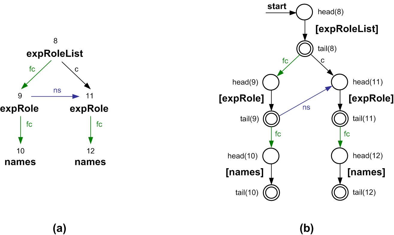
Definition 3.4 (Axis Graph Automaton)

Let $\mathcal{A}=(\mathit{Inst},$ $Axes,$ $Label,$ $\lambda)$ be an axis graph and $v$ a node in $\mathcal{A}$ . The axis graph automaton of $\mathcal{A}$ from $v$ , $\mathcal{M}_{\mathcal{A}}(v)=\{Q,\Sigma,\delta,q_{0},F\}$ , is an automaton [HU79] defined as follows:

•

For each node $w\in Inst$ there is a state $head(w)\in Q$ , a state $tail(w)\in Q$ and a transition $\delta(head(w),[\lambda(w)])=tail(w)$ ;
•

For each edge $(w_{i},w_{j})$ labeled $axis$ in $\mathcal{A}$ there is a transition $\delta(tail(w_{i}),axis)=head(w_{j})$ ;
•

All $tail(w)$ states in $Q$ , $w\in Inst$ , are final states in $F$ , and $head(v)$ is the initial state $q_{0}$ .

$\Box$

Example 3.3

Consider node $8$ of our running example. Figure 3.2 shows on the left hand side a fragment of the axis graph that contains node 8. The axis graph automaton from node $8$ (on the right hand side of the figure) has $head(8)$ as initial state and all $tail$ states as final. Each node in the axis graph fragment is unfolded into a head and a tail states in the automaton and its label is represented by a transition between them. Consider node $11$ with label $expRole$ that has $ns$ and $c$ incoming edges and a $\mathit{fc}$ outgoing edge in the axis graph. In the automaton, $11$ is represented by a $head(11)$ state that has $ns$ and $c$ incoming transitions and an outgoing transition $[expRole]$ to $tail(11)$ . The outgoing $\mathit{fc}$ edge is translated into a $\mathit{fc}$ transition from $tail(11)$ to the head state of the corresponding node, which is $12$ . $\Box$

An automaton can be obtained from an AxPRE following the usual Thompson’s construction for regular expressions with a minor change to the basis steps to account for AxPRE semantics (which require accepting all prefixes of the language). The language accepted by the so called AxPRE automaton thus constructed will always be prefix-closed. (A language $L$ is said to be prefix-closed if, given any word $l\in L$ , all prefixes of $l$ are also in $L$ [HU79].)

Definition 3.5 (AxPRE Automaton)

Let $\alpha$ be an AxPRE. The AxPRE automaton of $\alpha$ is an automaton $\mathcal{M}_{\alpha}$ obtained from $\alpha$ with a modified Thompson’s construction [HU79] for accepting all prefixes (Figure 3.3), in which only the final states of the basis rules are kept as final in the resulting automaton (the inductive rules for concatenation, disjunction and Kleene closure do not mark any additional state as final). The transition function $\hat{\delta}(q_{\alpha},axis)$ returns the states that can be reached by an $axis$ transition after following an arbitrary number (possibly zero) of $\epsilon$ transitions. $\Box$

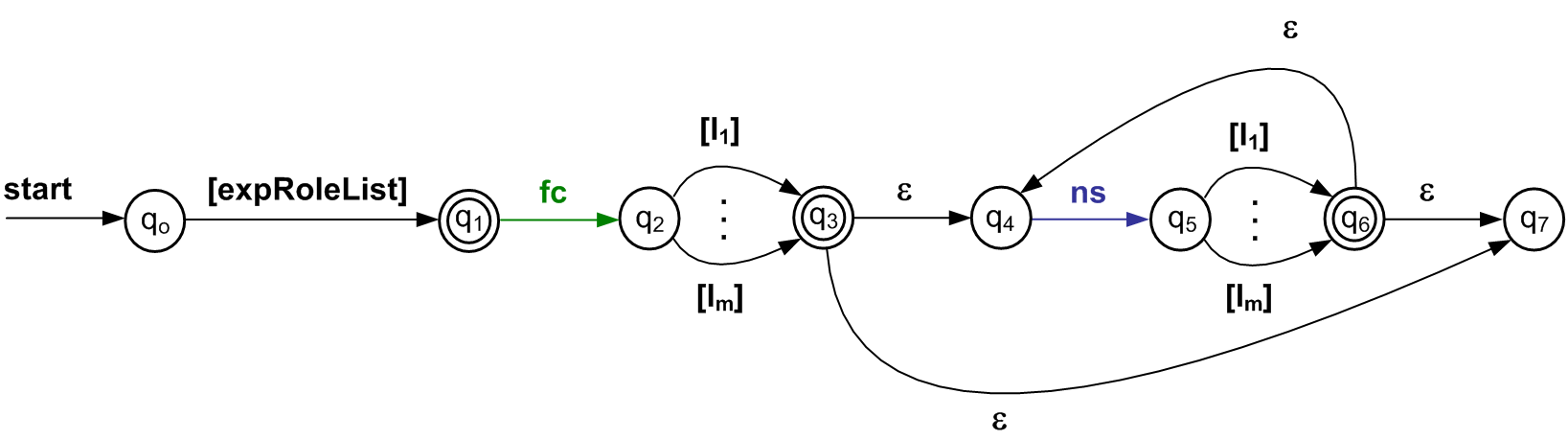
Example 3.4

Consider the AxPRE $[expRoleList].\mathit{fc}.ns^{*}$ and its automaton in Figure 3.4. The application of rule $axis[l]$ of the modified Thompson’s construction creates states $q_{0}$ , $q_{1}$ and the $[expRoleList]$ transition between them. The application of rule $axis$ creates $q_{2}$ , $q_{3}$ , $q_{5}$ , $q_{6}$ , and the $[l_{1}],\ldots,[l_{m}]$ transitions from $q_{2}$ to $q_{3}$ and from $q_{5}$ to $q_{6}$ (there is one transition $[l_{i}]$ for each string in $Label$ ). The final automaton is obtained by applying the concatenation and Kleene closure rules. $\Box$

An automaton for the intersection of two languages can be constructed by taking the product of the automata for the two languages [MW95, Yan90].

Definition 3.6 (Intersection Automaton)

Let $\mathcal{M}_{\mathcal{A}}(v)$ be the automaton of an axis graph $\mathcal{A}$ from a node $v$ , and $\mathcal{M}_{\alpha}$ be the automaton of an AxPRE $\alpha$ . The intersection automaton $\mathcal{M}_{\mathcal{A}}(v)\cap\mathcal{M}_{\alpha}$ is an automaton in which states are pairs $(q_{\mathcal{A}},$ $q_{\alpha})$ consisting of a state $q_{\mathcal{A}}\in\mathcal{M}_{\mathcal{A}}(v)$ and a state $q_{\alpha}\in\mathcal{M}_{\alpha}$ , and there is a transition $\delta((q_{\mathcal{A}},$ $q_{\alpha}),\mathcal{X})=(q^{\prime}_{\mathcal{A}},$ $q^{\prime}_{\alpha})$ if there are transitions $\delta(q_{\mathcal{A}},\mathcal{X})=q^{\prime}_{\mathcal{A}}$ in $\mathcal{M}_{\mathcal{A}}(v)$ and $\hat{\delta}(q_{\alpha},\mathcal{X})=q^{\prime}_{\alpha}$ in $\mathcal{M}_{\alpha}$ , where $\mathcal{X}$ is either an axis or a label. A state $\langle q_{\mathcal{A}},q_{\alpha}\rangle$ is final (initial) if both $q_{\mathcal{A}}$ and $q_{\alpha}$ are final (initial). $\Box$

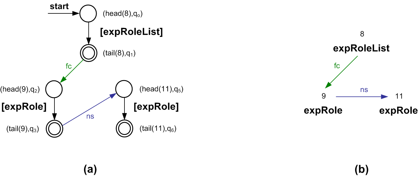
The machinery introduced in Definitions 3.4 through 3.6 is required for computing AxPRE neighbourhoods of nodes in the axis graph. The neighbourhood of a node $v$ by $\alpha$ can be obtained by taking the intersection between the axis graph automaton from $v$ and the AxPRE automaton of $\alpha$ , and then converting the resulting automaton to an axis graph fragment as described in Definition 3.7.

Definition 3.7 (AxPRE Neighbourhood of a Node)

Let $\mathcal{A}=(\mathit{Inst},$ $Axes,$ $Label,$ $\lambda)$ be an axis graph, $v$ a node in $\mathcal{A}$ , $\alpha$ an AxPRE, and $\mathcal{M}_{\mathcal{A}}(v)\cap\mathcal{M}_{\alpha}$ the intersection automaton of $\mathcal{M}_{\mathcal{A}}(v)$ and $\mathcal{M}_{\alpha}$ . The AxPRE neighbourhood of $v$ by $\alpha,$ denoted $\mathcal{N}_{\alpha}(v),$ is the subgraph of $\mathcal{A}$ defined as follows:

•

For each transition $\delta((head(w),q_{\alpha}),l)=(tail(w),q^{\prime}_{\alpha})$ , where $(tail(w),q^{\prime}_{\alpha})$ is a final state, there is a node $w$ with label $l$ in $\mathcal{A}$ ;
•

For each transition $\delta((tail(w_{i}),q_{\alpha}),axis)=(head(w_{j}),q^{\prime}_{\alpha})$ , where $(tail(w_{i}),q_{\alpha})$ is a final state, there is an edge $(w_{i},w_{j})$ labeled $axis$ in $\mathcal{A}$ .

$\Box$

Example 3.5 (AxPRE Neighbourhood of a Node)

Consider node 8 of our running example. The intersection automaton $\mathcal{M}_{\mathcal{A}}(8)$ $\cap$ $\mathcal{M}_{[expRoleList].\mathit{fc}.ns^{*}}$ is depicted in Figure 3.5 (a). States are labeled by pairs $(q_{\mathcal{A}},q_{\alpha})$ , where $q_{\mathcal{A}}$ is a state in automaton $\mathcal{M}_{\mathcal{A}}(8)$ and $q_{\alpha}$ is a state in automaton $\mathcal{M}_{[expRoleList].\mathit{fc}.ns^{*}}$ . The intersection has been computed following Definition 3.6. The figure shows only the states that have some incoming or outgoing transition. Note that transition $c$ between $tail(8)$ and $head(11)$ is not part of the intersection because $\mathit{fc}$ is the only outgoing transition from $q_{1}$ in $q_{\alpha}$ .

Figure 3.5 (b) shows the AxPRE neighbourhood of node 6, $\mathcal{N}_{[participant]c.\mathit{fc}.ns^{*}}(6)$ , obtained by converting the intersection automaton to an axis graph fragment as described in Definition 3.7. Note that transitions from $(head(v),\ldots)$ to $(tail(v),\ldots)$ in the intersection are node labels in the AxPRE neighbourhood and that transitions from $(tail(v),\ldots)$ to $(head(w),\ldots)$ are edge labels (axes) in the neighbourhood.

Consider now the five $[participant].c.\mathit{fc}.ns^{*}$ neighbourhoods depicted in Figure 3.6. Neighbourhood (a) matches a prefix of the AxPRE ( $[participant].c$ ) whereas (b) through (e) match the entire AxPRE but with a different number of iterations in the Kleene closure for $ns$ : 1 for (b) and (e), and 0 for (c) and (d). $\Box$

We formalize next the notion of AxPRE semantics based on AxPRE neighbourhoods.

Definition 3.8 (AxPRE Semantics)

Let $\mathcal{A}=(\mathit{Inst},$ $Axes,$ $Label,$ $\lambda)$ be an axis graph and $v$ a node in $\mathcal{A}$ . The evaluation of an AxPRE $\alpha$ on $v$ returns the AxPRE neighbourhood of $v$ by $\alpha$ . $\Box$

3.2 Neighbourhoods and bisimulation

AxPRE neighbourhoods allow us to define a notion of similarity between nodes in an axis graph. The idea underlying DescribeX is that nodes with similar AxPRE neighbourhoods will be grouped together. In particular, DescribeX uses the familiar concept of labeled bisimulation applied to AxPRE neighbourhoods, formalized by Definition 3.9.

Definition 3.9 (Labeled Bisimulation and Bisimilarity)

Let $\mathcal{N}_{\alpha}(v_{0})$ and $\mathcal{N}_{\beta}(w_{0})$ be two AxPRE neighbourhoods of an axis graph $\mathcal{A}=(\mathit{Inst},$ $Axes,$ $Label,$ $\lambda)$ , such that $Axes_{\alpha}\subseteq Axes$ and $Axes_{\beta}\subseteq Axes$ . A labeled bisimulation between $\mathcal{N}_{\alpha}(v_{0})$ and $\mathcal{N}_{\beta}(w_{0})$ is a symmetric relation $\approx$ such that for all $v\in\mathcal{N}_{\alpha}(v_{0})$ , $w\in\mathcal{N}_{\beta}(w_{0})$ , $E_{i}^{\alpha}\in Axes_{\alpha}$ , and $E_{i}^{\beta}\in Axes_{\beta}$ : if $v\approx w,$ then $\lambda(v)=\lambda(w)$ ; if $v\approx w,$ and $\langle v,v^{\prime}\rangle\in E_{i}^{\alpha}$ , then $\langle w,w^{\prime}\rangle\in E_{i}^{\beta}$ and $v^{\prime}\approx w^{\prime}$ . Two nodes $v\in\mathcal{N}_{\alpha}(v_{0})$ , $w\in\mathcal{N}_{\beta}(w_{0})$ are bisimilar, in notation $v\sim w$ , iff there exist a labeled bisimulation $\approx$ between $\mathcal{N}_{\alpha}(v_{0})$ and $\mathcal{N}_{\beta}(w_{0})$ such that $v\approx w$ . Similarly, two neighbourhoods $\mathcal{N}_{\alpha}(v_{0})$ and $\mathcal{N}_{\beta}(w_{0})$ are bisimilar, in notation $\mathcal{N}_{\alpha}(v_{0})\sim\mathcal{N}_{\beta}(w_{0})$ , iff $v_{0}\sim w_{0}$ . $\Box$

Definition 3.9 captures outgoing label paths from the nodes. Bisimulation provides a way of computing a double homomorphism between graphs. The widespread use of bisimulation in summaries is motivated by its relatively low computational complexity properties. The bisimulation contraction of a labelled graph can be done in time $O(m\log n)$ (where $m$ is the number of edges and $n$ is the number of nodes in a labelled graph) as shown in [PT87], or even linearly for acyclic graphs, as shown in [DPP04]. Using bisimulation also allows us to capture all the existing bisimulation-based proposals in the literature (Chapter 4).

Example 3.6

Let us consider the nodes $6$ and $18$ in the axis graph of Figure 3.1. Their $[participant].c.\mathit{fc}.ns^{*}$ neighbourhoods are depicted in Figure 3.6 (b) and (c), respectively. Based on Definition 3.9, we can define a labeled bisimulation $\approx$ between nodes $7$ and $19$ because they have the same labels and they do not have outgoing edges. For the same reasons we have $11\approx 21$ . However, it is not possible to define a labeled bisimulation between $9$ and $21$ because, even though they have the same labels, $9$ has one outgoing edge whereas $21$ does not. Thus, $9\not\approx 21$ . This prevents us from defining a label bisimulation between $8$ and $20$ because they each have only one outgoing $\mathit{fc}$ edge, but to nodes $9$ and $20$ , which are not bisimilar. Therefore, $8\not\approx 20$ . Similarly, $6\not\approx 18$ because they have edges with the same labels ( $c$ ) to nodes that are not bisimilar ( $8$ and $20$ ). Consequently, neighbourhoods (b) and (c) of Figure 3.6 are not bisimilar.

In contrast, let us compare now nodes $6$ and $18$ but with respect to their $[participant].c^{*}$ neighbourhoods, which are depicted in Figure 3.7 (b) and (c), respectively. In this case we can have $9\approx 21$ and $11\approx 21$ because all of them are leaves and have the same label. Therefore, $8\approx 20$ because the outgoing edges from $8$ go to nodes $9$ and $11$ , which are bisimilar to the target node ( $21$ ) of the only outgoing edge from $20$ . Thus, $6\approx 18$ because they have edges with the same labels ( $c$ ) to nodes that in this case are bisimilar ( $7\approx 19$ and $8\approx 20$ ). Consequently, neighbourhoods (b) and (c) of Figure 3.7 are in fact bisimilar. $\Box$

Definition 3.10 (AxPRE Bisimilarity)

Let $\mathcal{A}=(\mathit{Inst},$ $Axes,$ $Label,$ $\lambda)$ . When two nodes $v_{0}$ and $w_{0}$ in $\mathcal{A}$ have bisimilar neighbourhoods by the same AxPRE $\alpha$ , that is $\mathcal{N}_{\alpha}(v_{0})\sim\mathcal{N}_{\alpha}(w_{0})$ , we say that $v_{0}$ and $w_{0}$ are AxPRE bisimilar by $\alpha$ or $\alpha$ -bisimilar, in notation $v_{0}\sim^{\alpha}w_{0}$ . $\Box$

Example 3.7

Consider again the neighbourhoods in Figure 3.6. Nodes $6$ and $18$ have non-bisimilar $[participant].c.\mathit{fc}.ns^{*}$ neighbourhoods and thus $6\not\sim^{\alpha}18$ , where AxPRE $\alpha=[participant].c.\mathit{fc}.ns^{*}$ . However, if we consider now their $[participant].c^{*}$ neighbourhoods, which are bisimilar, then $6\sim^{\alpha^{\prime}}18$ for AxPRE $\alpha^{\prime}=[participant].c^{*}$ . $\Box$

AxPRE bisimilarity is used for defining partitions of an axis graph. Intuitively, a so called AxPRE partition assigns two nodes $v$ and $w$ in an axis graph to the same class if their AxPRE neighbourhoods by a given $\alpha$ are bisimilar. This is formalized by Definition 3.11.

Definition 3.11 (AxPRE Partition)

Let $\mathcal{A}=(\mathit{Inst},$ $Axes,$ $Label,$ $\lambda)$ be an axis graph and $\alpha$ an AxPRE. An AxPRE partition of $\mathit{Inst}$ by $\alpha$ , denoted $\mathcal{P}_{\alpha}$ , is a set of pairwise disjoint subsets of $\mathit{Inst}$ whose union is $\mathit{Inst}$ defined as follows: two nodes $v,w\in\mathit{Inst}$ belong to the same set $P_{\alpha}^{i}\in\mathcal{P}_{\alpha}$ iff $v\sim^{\alpha}w$ .

Definition 3.12 (Positive Classes)

Let $\mathcal{A}=(\mathit{Inst},$ $Axes,$ $Label,$ $\lambda)$ be an axis graph, $\alpha$ an AxPRE and $P_{\alpha}^{\emptyset}=\{v\in\mathit{Inst}\;|\;\mathcal{N}_{\alpha}(v)=\emptyset\}$ the set of the empty neighbourhoods in the AxPRE partition of $\mathit{Inst}$ by $\alpha$ . Then, $\mathcal{P}^{+}_{\alpha}=\mathcal{P}_{\alpha}-P_{\alpha}^{\emptyset}$ is the set of positive classes of $\mathcal{P}_{\alpha}$ . $\Box$

Since all nodes that have an empty AxPRE neighbourhood belong to the same equivalence class, $\mathcal{P}_{\alpha}$ and $\mathcal{P}^{+}_{\alpha}$ differ in at most one set.

Example 3.8

Consider the AxPRE partitions by $[l_{1}],\ldots,[l_{n}]$ , where $l_{1},\ldots,l_{n}$ are the different node labels that appear in the axis graph, have one positive class each because each neighbourhood represents a different node label. (Note that the $n$ different positive classes do not overlap.) Moreover, the union of those $n$ sets (each coming from a different partition) also constitute a partition of $\mathit{Inst}$ . In contrast, if we take only a proper subset of $m$ node labels, $m<n$ , the $m$ positive classes of the resulting AxPRE partitions do not constitute a partition because their union does not have all nodes in $\mathit{Inst}$ . $\Box$

Given an AxPRE, the positive classes plus one additional class for the empty neighbourhood forms a partition. If we have another AxPRE whose positive classes fall exclusively within this empty neighbourhood class, then these two AxPREs may be used together to summarize an axis graph. We are interested in sets of AxPREs whose positive classes define a partition of $\mathit{Inst}$ , which is formalized next.

Definition 3.13 (Positive Partition)

Let $\mathcal{A}=(\mathit{Inst},$ $Axes,$ $Label,$ $\lambda)$ be an axis graph. A set $\mathbb{A}=\{\alpha_{1},\ldots,\alpha_{n}\}$ of AxPREs defines a positive partition of $\mathcal{A}$ , denoted $\mathcal{P}_{\mathbb{A}}$ , iff $\bigcup_{i}\mathcal{P}^{+}_{\alpha_{i}}$ is a partition of $\mathit{Inst}$ . $\Box$

The intuition behind the notion of positive partition from a set of AxPREs $\mathbb{A}=\{\alpha_{1},\ldots,\alpha_{n}\}$ can be explained as follows. We know, by Definition 3.13, that each $\alpha_{i}$ in $\mathbb{A}$ defines an AxPRE partition which has positive classes and a unique empty neighbourhood class. In order for the set $\mathbb{A}$ to define a positive partition, the empty neighbourhood class of $\alpha_{i}$ has to be further partitioned by some $\alpha_{j}$ in $\mathbb{A}$ . In other words, when the entire set $\mathbb{A}$ is considered, every node that belongs to the empty neighbourhood of some $\alpha_{i}$ also belongs to some positive class of some $\alpha_{j}$ .

Example 3.9 (Positive Partition)

Positive partitions play a key role in our framework. This requires a thorough understanding of the semantics of the AxPREs, and the partitions they define. We discuss now some particular cases of our running example of Figure 3.1.

Let us consider first the AxPRE $\epsilon$ , which evaluated on each axis graph node will produce as many different neighborhoods as there are different labels in the axis graph (each neighbourhood containing a single node). Since all nodes with bisimilar neighbourhoods will belong to the same class, if there are $n$ different labels in the axis graph the $\epsilon$ positive partition will contain $n$ classes (Figure 3.8 shows below each SD node the sets of the partition for our running example). The same positive partition can be obtained with the set of expressions $\mathbb{A}=\{[l_{1}],\ldots,[l_{n}]\}$ , where $l_{1},\ldots,l_{n}$ are all the different node labels that appear in the axis graph. In our running example, the set of expressions equivalent to $\epsilon$ would contain $[interaction]$ , $[participant]$ , etc.

Let us consider now the AxPRE $[participant].$ The partition by $[participant]$ is obtained as follows: for each node in the axis graph, we compute the AxPRE neighbourhood corresponding to $[participant]$ , and all nodes with bisimilar neighbourhoods (i.e., all nodes that are $[participant]$ -bisimilar) will belong to the same class. Thus, the partition will consist of two classes: one containing all the nodes $v$ such that $\lambda(v)=participant,$ which is the set $\{4,6,18,23,28\}$ (the positive class), and the other one with the remaining nodes (the empty neighbourhood class). On the other hand, the $[\neg participant]$ partition will create as many classes as nodes $v$ with labels $\lambda(v)\neq participant$ exist in $\mathit{Inst}$ . In our running example, the $[\neg participant]$ partition will have nine positive classes (one per label different from “participant”) whereas all nodes with “participant” label will belong to the empty neighbourhood class. The two AxPREs $[participant]$ and $[\neg participant]$ , when put together, define a positive partition with ten classes (one for each label). $\Box$

3.3 Describing summaries with AxPREs

In the previous sections, we have introduced the basic machinery we need to define summary descriptor (SD, for short). An SD is defined from an axis graph and a set of AxPREs. Intuitively, an SD consists of an axis graph in which each node has associated an AxPRE and a set in its AxPRE partition, and whose edges represent axis relationships between those sets.

Definition 3.14 (Summary Descriptor)

Let $\mathcal{A}=(\mathit{Inst},$ $Axes,$ $Label,$ $\lambda)$ be an axis graph of an instance. A summary descriptor (SD for short) of $\mathcal{A}$ is a structure $\mathcal{D}_{\mathbb{A}}=(\mathbb{A},\mathcal{G},axpre,extent)$ that consists of:

•

a set $\mathbb{A}=\{\alpha_{1},\ldots,\alpha_{n}\}$ of AxPREs such that $\mathcal{P}_{\mathbb{A}}$ is a positive partition of $\mathcal{A}$ by $\mathbb{A}$ ;
•
an axis graph $\mathcal{G}=(Sum,Axes^{\mathcal{D}},Label,\lambda^{\mathcal{D}})$ , called SD graph, representing axis relationships between nodes in the sets (extents) of the positive partition $\mathcal{P}_{\mathbb{A}}$ where:
- –
  
  $Sum$ is a set of nodes;
- –
  
  $Axes^{\mathcal{D}}$ is a set of binary relations $\{E_{1}^{\mathcal{D}},\ldots,E_{n}^{\mathcal{D}}\}$ in $Sum\times Sum$ such that there is a tuple $\langle s_{j},s_{k}\rangle$ in $E_{i}^{\mathcal{D}}$ iff $\exists E_{i}^{\mathcal{A}}\in Axes,\exists v\in extent(s_{j}),\exists w\in extent(s_{k})\wedge\langle v,w\rangle\in E_{i}^{\mathcal{A}}$ (edges are labeled by axis names);
- –
  
  $Label$ is the set of node labels from $\mathcal{A}$ ;
- –
  
  $\lambda^{\mathcal{D}}$ is a function that assigns labels in $Label$ to nodes in $Sum$ .
•

a bijective function $axpre$ that assigns AxPREs from $\mathbb{A}$ to nodes in $Sum$ ;
•

a bijective function $extent$ that assigns a set from the positive partition $\mathcal{P}_{\mathbb{A}}$ to each node in $Sum$ (the set assigned is called the extent of the node).

$\Box$

An SD has some particular characteristics. The set $\mathbb{A}$ uniquely defines the extents of the SD, and therefore its nodes, for any particular axis graph instance. In other words, given an axis graph $\mathcal{A}$ and the set $\mathbb{A}$ we can create the SD of $\mathcal{A}$ by $\mathbb{A}$ . On the other hand, not any set of AxPREs define a positive partition and thus an SD. The first SDs we can distinguish are those that are defined by a unique AxPRE from those that have a multi-AxPRE definition. We denote the former ones as homogeneous SDs because all their nodes are defined uniformly. Homogeneous SDs are the most common in the summary literature (e.g., dataguides [GW97], 1-index [MS99], ToXin [RM01], A(k)-index [KSBG02], F&B-Index [KBNK02], Skeleton [BCF+05]). SDs defined by multiple AxPREs are called heterogeneous.

Definition 3.15 (Homogeneous and Heterogeneous SDs)

When the extents of all nodes in a SD $\mathcal{D}$ are defined with the same AxPRE $\alpha$ (i.e., $|\mathbb{A}|=1$ ), we say that the corresponding SD is homogeneous. In this case we say that $\mathcal{D}$ is an $\alpha$ SD. In contrast, if at least two different nodes are defined with different AxPREs (i.e., $|\mathbb{A}|>1$ ) we have a heterogeneous SD. $\Box$

Proposition 3.1

Given an axis graph $\mathcal{A}$ , and a set $\mathbb{A}$ of AxPREs. If each $\alpha_{i}\in\mathbb{A}$ contains only AxPREs of the form $[l],l\in Label$ different from each other, such that there is an AxPRE for each label in $\mathcal{A},$ then $\mathbb{A}$ defines an heterogeneous SD. Such an SD is denoted label SD. $\Box$

Proof 3.1

It is easy to see that if $\mathbb{A}$ contains all the labels in $\mathcal{A}$ , each AxPRE $[l]$ will create a positive class labeled $P_{l}$ associated to a different SD node $s_{l}$ such that all nodes in $\mathcal{A}$ with label $l$ will belong to the extent of $s_{l}.$ Since $\mathbb{A}$ contains all the labels in the document, the set $P=\bigcup_{i}\mathcal{P}^{+}_{\alpha_{i}}$ will be a partition of $\mathit{Inst}$ . $\Box$

Note that we need to know the instance in advance in order to define the set $\mathbb{A}$ accordingly. However, the label SD can also be defined by the AxPRE $\epsilon$ , which makes the label SD homogeneous and its definition independent of the axis graph. The $\epsilon$ SD will produce exactly the same equivalence classes that the set $\mathbb{A}$ of Proposition 3.1.

Example 3.10 (Summary Descriptor)

Figure 3.8 shows a label SD for our running example. Since there are ten different labels in the axis graph of the instance, there are ten summary nodes in the label SD. Nodes in the figure are labeled by their AxPREs, so we are considering a heterogeneous label SD in which $\mathbb{A}$ contains an AxPRE per label. The extent of each node is depicted below it. Edges represent summary axis relations. For instance, there is an edge from $s_{2}$ to $s_{10}$ labeled $c,$ because there is a $c$ edge in the axis graph from node 14 (in the extent of $s_{2}$ ) to node 16 (in the extent of $s_{10}$ ).

There are three kinds of edges in the figure, depending on properties of the sets that participate in the axis relation: dashed, regular, and bold. Dashed edges, like $(s_{2},s_{10})$ with label $c$ , mean that some element in the extent of $s_{2}$ has a child in the extent of $s_{10}$ . Regular edges, like ( $s_{6},s_{7}$ ) with label $\mathit{fc}$ , mean that every element in the extent of $s_{6}$ has a first child in the extent of $s_{7}$ . (Since $c$ includes $\mathit{fc}$ , we do not draw a $c$ edge when an $\mathit{fc}$ edge exists.) Finally, bold edges, like $(s_{4},s_{5})$ with label $\mathit{fc}$ , mean that every element in the extent of $s_{5}$ is a first child of some element in the extent of $s_{4}$ and that every element in the extent of $s_{4}$ has a first child in the extent of $s_{5}.$ The nodes and edges in the figure constitute the SD graph of the label SD.

Figure 3.9 shows another heterogeneous SD with a different set $\mathbb{A}$ where $[participant]$ , $[expRoleList]$ and $[expRole]$ from Figure 3.8 have been replaced by $[participant].c.\mathit{fc}.ns^{*}$ , $[expRoleList].\mathit{fc}.ns^{*}$ and $[expRole].ns^{*}$ , respectively. $\Box$

Definition 3.16 (Summary Axis Stability)

Let $e=\langle s_{i},s_{j}\rangle$ be an SD graph edge with label $axis$ . We say that $e$ is an existential edge if $\exists x\in extent(s_{i}),\exists y\in extent(s_{j})\wedge\langle x,y\rangle\in axis$ , and a forward-stable edge if $\forall x\in extent(s_{i}),\exists y\in extent(s_{j})\wedge\langle x,y\rangle\in axis$ . $\Box$

Definition 3.16 captures the relationship between edges in the SD graph and the axis graph, and generalizes to several axes the edge stability representation in XSketch [PG06b]. Note that all forward-stable edges are also existential. In Figures 3.8 and 3.9, existential edges are represented by dashed lines and forward-stable edges by solid lines. A dashed line does not necessarily mean that an edge is not forward-stable, it might be that stability has not been checked on that edge (existential edges in Figures 3.8 and 3.9 have been checked and are not forward-stable). When an edge $e$ and its inverse are both forward-stable, $e$ is shown in bold lines.

Algorithm 3.1 computes an SD $D$ from an axis graph $A$ and a set $X$ of AxPREs that define a positive partition of $A$ . Essentially, the algorithm creates the positive partition in one pass over $A$ (outer loop spanning steps 2-18). Loop 3-18 computes the AxPRE neighbourhood of $v$ for each $\alpha$ in $X$ (step 5) in order to find the $\alpha$ for which the AxPRE neighbourhood of $v$ is non-empty. Since $X$ defines a positive partition as a precondition, then for every $v$ there is one and only one $\alpha$ in $X$ such that $\mathcal{N}_{\alpha}(v)\neq\emptyset$ . This guarantees that condition in step 6 is true exactly once for every $v$ in $A$ .

The next task in the algorithm is to find the extent where $v$ belongs. Loop 7-11 compares by bisimulation $\mathcal{N}_{\alpha}(v)$ with every node in $D$ that has the same AxPRE $\alpha$ . If there is a node $s$ in $D$ with $\alpha$ but the $\alpha$ neighbourhoods of $v$ and $s$ are not bisimilar (step 10), then a new node $s$ is created and $v$ is added to its extent (steps 12-16). The same happens if there is no $s$ in $D$ with $\alpha$ at all. Since each $v$ in $A$ may be in an $axis$ relationship with nodes in any extent, the final loop 17-18 checks edge existence (for the input set of axes $Axes^{\mathcal{D}}$ ) between the node $s$ such that $v\in extent(s)$ and every other node in $D$ . The result of the algorithm is an SD $D$ where each $s$ in $D$ has associated a set in the positive partition of $A$ by $X$ and the axes in $Axes^{\mathcal{D}}$ satisfy the conditions in Definition 3.16.

As shown, loop 2-18 performs $|\mathit{Inst}|$ iterations. At any given moment, there is at most the same number of nodes in $D$ as in $A$ (each extent having only one node) and all have the same AxPRE. Therefore, loop 7-11 performs $|\mathit{Inst}|$ iterations in the worst case. Each iteration computes an AxPRE bisimulation (step 10) with time complexity $O(m.log|\mathit{Inst}|)$ , where $m$ is the total number of tuples (edges) in all axes in $Axis$ . The worst case for loop 17-18 is the same as that of loop 7-11, so it also performs $|\mathit{Inst}|$ iterations. Thus, the total time complexity of Algorithm 3.1 is $O(|\mathit{Inst}|.m.log|\mathit{Inst}|)$ .

Algorithm 3.1

createSD $(A,X)$
Input: An axis graph $A$ , a set $X$ of AxPREs that defines a positive partition of $A$ , and a set $Axes^{\mathcal{D}}$ of SD axes where each axis contains only the empty tuple
Output: An SD $D$

1: create empty SD

D

2: for every

v

A

candidate:=\emptyset

4: for every

\alpha

X

5: compute the

\alpha

neighbourhood of

v

\mathcal{N}_{\alpha}(v)

6: if

\mathcal{N}_{\alpha}(v)\neq\emptyset

then

7: for every node

s

D

such that

axpre(s):=\alpha

8: let

w

be a node in

extent(s)

9: compute the

\alpha

neighbourhood of

w

\mathcal{N}_{\alpha}(w)

10: if

v\sim^{\alpha}w

(i.e.,

\mathcal{N}_{\alpha}(v)\sim\mathcal{N}_{\alpha}(w)

) then

11:

candidate:=s

12: if

candidate=\emptyset

then

13: create a new node

candidate

D

14:

axpre(candidate):=\alpha

15:

\lambda^{D}(candidate):=\lambda(v)

16: add

v

extent(s)

17: for every node

s^{\prime}\neq s

D

18: add tuple

\langle s,s^{\prime}\rangle

and

\langle s^{\prime},s\rangle

to the corresponding

axis

Axes^{\mathcal{D}}

if conditions in Definition 3.16 are satisfied

The notion of an AxPRE neighbourhood can also be defined for an SD graph, and it is called summary AxPRE neighbourhood of a node. Since an SD Graph is in fact an axis graph $\mathcal{G}=(Sum,Axes^{\mathcal{D}},Label,\lambda^{\mathcal{D}})$ , for any given SD node $s$ and AxPRE $\alpha$ we can define its SD graph automaton $\mathcal{M}_{\mathcal{G}}(s)$ (Definition 3.4) and intersect it with the AxPRE automaton $\mathcal{M}_{\alpha}$ (Definition 3.5) in order to obtain an AxPRE neighbourhood (Definition 3.7) of $s$ .

Definition 3.17 (Summary Neighbourhood)

Let $\mathcal{D}_{\mathbb{A}}=(\mathbb{A},$ $\mathcal{G},$ $axpre,$ $extent)$ be an SD, axis graph $\mathcal{G}=(Sum,$ $Axes^{\mathcal{D}},$ $Label,$ $\lambda^{\mathcal{D}})$ its SD graph, $s$ a node in $\mathcal{G}$ , $\alpha$ an AxPRE, and $\mathcal{M}_{\mathcal{G}}(s)\cap\mathcal{M}_{\alpha}$ the intersection automaton of $\mathcal{M}_{\mathcal{G}}(s)$ and $\mathcal{M}_{\alpha}$ . The summary neighbourhood of $s$ by $\alpha$ , denoted $\mathcal{N}^{\mathcal{G}}_{\alpha}(s),$ is the subgraph of $\mathcal{G}$ as in Definition 3.7. $\Box$

Definition 3.18 (Partition Refinement)

Let $\mathcal{A}=(\mathit{Inst},$ $Axes,$ $Label,$ $\lambda)$ be an axis graph. If $\mathcal{P}_{\mathbb{A}}$ and $\mathcal{P}_{\mathbb{B}}$ are positive partitions of $\mathcal{A}$ , $\mathcal{P}_{\mathbb{A}}$ is a partition refinement of $\mathcal{P}_{\mathbb{B}}$ if every set of $\mathcal{P}_{\mathbb{A}}$ is contained in a set of $\mathcal{P}_{\mathbb{B}}$ . $\Box$

Definition 3.19 (SD Refinement)

Let $\mathcal{A}=(\mathit{Inst},$ $Axes,$ $Label,$ $\lambda)$ be an axis graph and $\mathcal{D}_{\mathbb{A}}=(\mathbb{A},\mathcal{G},extent)$ and $\mathcal{D}_{\mathbb{B}}=(\mathbb{B},\mathcal{G}^{\prime},extent^{\prime})$ be two SDs of $\mathcal{A}$ . $\mathcal{D}_{\mathbb{A}}$ is an SD refinement of $\mathcal{D}_{\mathbb{B}}$ if $\mathcal{P}_{\mathbb{A}}$ is a partition refinement of $\mathcal{P}_{\mathbb{B}}$ . $\Box$

Proposition 3.2

Let $\mathcal{A}=(\mathit{Inst},$ $Axes,$ $Label,$ $\lambda)$ be an axis graph, $\alpha$ and $\beta$ be AxPREs, and $\mathcal{P}_{\alpha}$ and $\mathcal{P}_{\beta}$ be AxPRE partitions of $\mathcal{A}$ . If $\alpha$ is contained in $\beta$ then $\mathcal{P}_{\beta}$ is a refinement of $\mathcal{P}_{\alpha}$ . $\Box$

Proof 3.2

(sketch) The proof follows from the notion of AxPRE neighbourhoods. If $\alpha$ is contained in $\beta$ then for any given node $v$ , its $\alpha$ neighbourhood is contained in its $\beta$ neighbourhood. Consequently, two nodes that are not distinguished by $\alpha$ (i.e., they are $\alpha$ -bisimilar) may be distinguished by $\beta$ , but not the other way around. This guarantees that $\beta$ creates either the same partition as $\alpha$ or a refinement. $\Box$

Corollary 3.1

Let $\mathcal{A}=(\mathit{Inst},$ $Axes,$ $Label,$ $\lambda)$ be an axis graph and $\mathcal{D}_{\mathbb{A}}=(\mathbb{A},\mathcal{G},extent)$ and $\mathcal{D}_{\mathbb{B}}=(\mathbb{B},G^{\prime},extent^{\prime})$ be two SDs of $\mathcal{A}$ . If every $\beta\in\mathbb{B}$ is contained in some $\alpha\in\mathbb{A}$ then $\mathcal{D}_{\mathbb{A}}$ is an SD refinement of $\mathcal{D}_{\mathbb{B}}$ . $\Box$

Example 3.11 (SD Refinement)

Let us consider the label SD of Figure 3.9. Recall that in the label SD, $\mathbb{A}=\{[l_{1}],...,[l_{n}]\},$ where $l_{i}\in Label,$ $l_{i}\neq l_{j}~\forall~i,j,$ and $\bigcup_{i}~{l_{i}}=Label.$ Suppose we want to refine node $s_{4}.$ For this node, the partition represented in the figure was produced by the AxPRE $[participant].$ If we replace this AxPRE by $[participant].c$ in $\mathbb{A},$ and apply this set of AxPREs to $Inst$ , two nodes will be produced, let us call these nodes $s_{41}$ and $s_{42},$ with extents $\{4\}$ and $\{6,18,23,28\}$ , respectively ( $s_{4}$ will not appear because the AxPRE which produced it was replaced by the new one). This occurs because node 4 in the axis graph has one child (namely interactorRef) while the other four nodes have two children each (interactorRef and expRoleList). Thus, applying $[participant]c$ we obtain two different AxPRE neighbourhoods, plus the empty neighbourhood, which is itself partitioned by the remaining AxPREs.

Analogously, if we want to refine the extent of $s_{42}$ further using the AxPRE $c.ns,$ we will replace the AxPRE $[participant].c$ by $[participant].c.c.ns.$ This will produce three sets, with extents: $\{4\},$ $\{6,28\},$ $\{18,23\}.$

Finally, suppose now that the label SD is defined using $\mathbb{A}=\epsilon,$ and we want to refine node $s_{4}$ with $[participant].c.$ In this case, just adding the new AxPRE does not suffice, because we would not obtain an SD: the union of positive partitions will not be a partition of $Inst$ because $\epsilon$ will still produce its own partitions. We solve this adding the AxPRE $[\neg participant],$ which will produce the remainder of the label SD and will send all nodes labeled $participant$ to the empty neighbourhood class. $\Box$

The notions of partition and SD refinement, besides describing the axis structure of an axis graph, allows us to define a hierarchy of SDs. This provides the basis for recognizing a lattice among different SDs, where each node corresponds to a different AxPRE definition. We will show that this lattice covers all the summaries addressed in the literature, plus more complex new ones. At the top of this hierarchy (i.e., the coarsest partition), the empty AxPRE defines a SD where each node is partitioned by label (as shown in Figure 4.1), a typical summary found in the literature [CM94, NUWC97]. The bottom of the lattice may vary, although the finest partition granularity can be represented by the expression $(\mathit{fc}.ns^{*})^{*},$ that produces a partition in which each node in the axis graph will belong to a different equivalence class.

Definition 3.20 (DescribeX Lattice)

A DescribeX lattice with respect to a set of axes $A=\{a_{1},\ldots,a_{n}\}$ is defined as follows: each node corresponds to an AxPRE generated by the grammar of Definition 3.3 when the terminal axis is one of $a_{1},...,a_{n}.$ Also, there is an edge $(n_{1},n_{2})$ in the lattice if and only if the AxPRE of $n_{2}$ is contained in the AxPRE of $n_{1}.$ $\Box$

From Definition 3.20 it follows that the coarsest partition that the lattice may define is the label SD. The finest partition depends on the chosen set of axes.

This chapter provided an overview of the DescribeX framework, including the AxPRE language and some fundamental notions like neighbourhood, bisimilarity, and summary descriptor (SD). In the next chapter we will discuss how the DescribeX lattice captures and generalizes many proposals in the literature.

Chapter 4 Capturing earlier literature proposals with DescribeX

DescribeX summaries can be classified in a lattice that describes a refinement relationship between entire summaries (Definition 3.20). In this chapter we revisit some of the related work discussed in Chapter 2 that can be captured in such a lattice by the DescribeX framework.

Figure 4.1 shows a fragment of a DescribeX summary lattice that captures earlier proposals based on the notion of bisimilarity (in green) and ad-hoc constructions (in red). Each node in the figure corresponds to a homogeneous SD defined by an AxPRE. DescribeX not only captures most summary proposals but also provides a declarative way of defining entirely new ones: nodes and edges in blue are a sample of the richer SDs that were never considered in the literature, like the one that appears in Figure 3.9 ( $c.\mathit{fc}.ns^{*}$ ) and in Chapter 8 ( $p^{*}|c.\mathit{fs}$ ).

4.1 Bisimilarity-based proposals

The earliest bisimilarity-based summary proposal is the family presented in [MS99], which contains a $p^{*}$ summary: the 1-index. The 1-index partition is computed by using bisimulation as the equivalence relation. The F&B-Index [KBNK02], is an example of a $(p|c)^{*}$ SD. The F&B-Index construction uses bisimulation like the 1-index, but applied to the edges and their inverses in a recursive procedure until a fix-point. With this construction, the F&B-Index’s equivalence classes are computed according to the incoming and outgoing label paths of the nodes. The same work introduces the F+B-index (a $p^{*}|c^{*}$ AxPRE summary constructed by applying bisimulation to the edges and their inverses only once) and the BPCI(k,j,m) index (a $(p^{k}|c^{j})^{m}$ AxPRE summary, where $k$ , and $j$ controls the lengths of the paths and $m$ the iterations of the bisimulation on the edges and their inverses). The F+B-index and the F&B-index are BPCI( $\infty,\infty,1$ ) and BPCI( $\infty,\infty,\infty$ ) respectively. The A(k)-index [KSBG02] is a $p^{k}$ AxPRE summary based on $k$ -bisimilarity (bisimilarity computed for paths of length $k$ ). Thus, the A(0)-index is a label SD, the A(1)-index is a $p$ SD, the A(2)-index is a $p.p$ SD, and the A(h)-index is the $p^{h}$ SD. We discuss some of these proposals in more detail.

Unlike standard definitions in the bisimulation literature [PT87, DPP04], 1-index, A(k)-index, F&B-index, and BPCI(k,j,m) use a bisimulation defined backwards in order to capture incoming paths to the nodes. We provide next a definition of backwards bisimulation and bisimilarity for completeness. In the literature, the only axes considered are $c$ and $\mathit{idref}$ .

Definition 4.1 (Backwards Bisimulation and Bisimilarity)

Let $\mathcal{G}_{1}$ and $\mathcal{G}_{2}$ be two rooted subgraphs of an axis graph $\mathcal{A}=(\mathit{Inst},$ $Axes,$ $Label,$ $\lambda)$ , such that $Axes_{\mathcal{G}_{1}}\subseteq Axes$ and $Axes_{\mathcal{G}_{2}}\subseteq Axes$ , and let $r_{1},r_{2}\in\mathit{Inst}$ be the roots of $\mathcal{G}_{1}$ and $\mathcal{G}_{2}$ respectively. A backwards bisimulation between $\mathcal{G}_{1}$ and $\mathcal{G}_{2}$ is a symmetric relation $\approx_{b}$ such that for all $v\in\mathcal{G}_{1}$ , $w\in\mathcal{G}_{2}$ , $E_{i}^{\mathcal{G}_{1}}\in Axes_{\mathcal{G}_{1}}$ , and $E_{i}^{\mathcal{G}_{2}}\in Axes_{\mathcal{G}_{2}}$ : if $v\approx_{b}w,$ then $\lambda(v)=\lambda(w)$ ; if $v\approx_{b}w,$ and $\langle v^{\prime},v\rangle\in E_{i}^{\mathcal{G}_{1}}$ , then $\langle w^{\prime},w\rangle\in E_{i}^{\mathcal{G}_{2}}$ and $v^{\prime}\approx_{b}w^{\prime}$ . Two nodes $v\in\mathcal{G}_{1}$ , $w\in\mathcal{G}_{2}$ are backward bisimilar, in notation $v\sim_{b}w$ , iff there exist a backwards bisimulation $\approx_{b}$ between $\mathcal{G}_{1}$ and $\mathcal{G}_{2}$ such that $v\approx_{b}w$ . $\Box$

It is easy to see that the backwards bisimulation is an equivalence relation. The F&B-Index construction uses backwards bisimulation like the 1-index, but applied to $c$ and $\mathit{idref}$ edges and their inverses. Algorithm 4.2 computes the equivalence classes for the F&B-Index according to both incoming and outgoing label paths of the nodes.

Algorithm 4.2

F&B $-construction(G)$
Input: Data graph $G$
Output: F&B-index $I$

1: let

\mathcal{P}

be a partition of the nodes in

G

\mathcal{P}\leftarrow

label SD partition of

G

3: repeat

4: reverse all edges in

G

\mathcal{P}\leftarrow

compute the backwards bisimilarity partition of

G

initializing the computation with

\mathcal{P}

6: reverse all edges in

G

, obtaining the original

G

\mathcal{P}\leftarrow

compute the backwards bisimilarity partition of

G

initializing the computation with

\mathcal{P}

8: until

\mathcal{P}

does not change (fix point)

9: for each equivalence class

P_{i}\in\mathcal{P}

10: create an index node

s\in I

11:

extent(s)\leftarrow P_{i}

12: for each edge from

v

w

G

13: let

s\in I

be an index node such that

v\in extent(s)

14: let

s^{\prime}\in I

be an index node such that

w\in extent(s)

15: if there is no edge from

s

s^{\prime}

then

16: create an edge from

s

s^{\prime}

Proposition 4.1

Let $G$ be an axis graph with $Axes=\{c\}$ (or $Axes=\{c,\mathit{idref}\}$ ). The F&B-index of $G$ is a $(p|c)^{*}$ SD (or a $(p|c|\mathit{idref}|\mathit{idref}^{-1})^{*}$ SD). $\Box$

Proof 4.1

The input data graph used in the F&B-index construction (Algorithm 4.2) can be viewed as an axis graph with the $c$ axis, in which the reversed edges of lines $4$ and $6$ correspond to the $c^{-1}$ axis (equivalent to a $p$ axis). Therefore, for simplicity, instead of reversing edges we use an axis graph $G$ with $Axes=\{c\}$ and take its inverse when necessary. If id-idrefs are considered, then $Axes=\{c,\mathit{idref}\}$ .

Let us consider first the case of $Axes=\{c\}$ . We start with the label SD in Line $2$ , which is an $\epsilon$ SD. Lines $4$ and $5$ are equivalent to refining all nodes in the initial $\epsilon$ SD by the $c^{*}$ AxPRE. This produces a $c^{*}$ SD. Then, lines $6$ and $7$ produce a refinement of all $c^{*}$ nodes by the $p^{*}$ AxPRE, thus obtaining a $c^{*}.p^{*}$ SD. The iterative process until the fix point can be represented in our framework as a Kleene closure of the $c^{*}.p^{*}$ AxPRE, which yields a $(c^{*}.p^{*})^{*}$ SD. It is easy to see that AxPRE $(c^{*}.p^{*})^{*}$ produces the same SD as $(p|c)^{*}$ (by identity of regular expressions). The remainder of the algorithm (lines $9$ - $16$ ) creates existential edges like in Definition 3.16.

When $Axes=\{c,\mathit{idref}\}$ , the argument is similar but with AxPREs $(c|\mathit{idref})^{*}$ and $(p|\mathit{idref}^{-1})^{*}$ instead of $c^{*}$ and $p^{*}$ , respectively. In this case, the final AxPRE for the SD is $(p|c|\mathit{idref}|\mathit{idref}^{-1})^{*}$ . $\Box$

The notion of k-bisimilarity used in the A(k)-index was defined to capture incoming paths on $c$ and $\mathit{idref}$ edges of length up to $k$ . We provide next a more general definition for axis graphs that supports paths on all types of axes.

Definition 4.2 (Backwards k-Bisimulation and k-Bisimilarity)

Let $\mathcal{G}_{1}$ and $\mathcal{G}_{2}$ be two rooted subgraphs of an axis graph $\mathcal{A}=(\mathit{Inst},$ $Axes,$ $Label,$ $\lambda)$ , such that $Axes_{\mathcal{G}_{1}}\subseteq Axes$ and $Axes_{\mathcal{G}_{2}}\subseteq Axes$ , and let $r_{1},r_{2}\in\mathit{Inst}$ be the roots of $\mathcal{G}_{1}$ and $\mathcal{G}_{2}$ respectively. A backwards k-bisimulation between $\mathcal{G}_{1}$ and $\mathcal{G}_{2}$ is a symmetric relation $\approx^{k}_{b}$ such that for all $v\in\mathcal{G}_{1}$ , $w\in\mathcal{G}_{2}$ , $E_{i}^{\mathcal{G}_{1}}\in Axes_{\mathcal{G}_{1}}$ , and $E_{i}^{\mathcal{G}_{2}}\in Axes_{\mathcal{G}_{2}}$ : if $v\approx^{0}_{b}w,$ then $\lambda(v)=\lambda(w)$ ; if $v\approx^{k}_{b}w,$ and $\langle v^{\prime},v\rangle\in E_{i}^{\mathcal{G}_{1}}$ , then $\langle w^{\prime},w\rangle\in E_{i}^{\mathcal{G}_{2}}$ and $v^{\prime}\approx^{k-1}_{b}w^{\prime}$ . Two nodes $v\in\mathcal{G}_{1}$ , $w\in\mathcal{G}_{2}$ are backward k-bisimilar, in notation $v\sim^{k}_{b}w$ , iff there exist a backwards k-bisimulation $\approx^{k}_{b}$ between $\mathcal{G}_{1}$ and $\mathcal{G}_{2}$ such that $v\approx^{k}_{b}w$ . $\Box$

Note that backwards k-bisimilarity defines an equivalence relation on the nodes in the axis graph. The partition created by the backwards k-bisimilarity corresponds to the A(k)-index, where $k$ is a parameter that represents the length of the incoming paths summarized by the index.

Algorithm 4.3

BPCI $-construction(G,k_{in},k_{out},td)$
Input: Data graph $G$ , local similarities $k_{in}$ and $k_{out}$ , tree depth $td$
Output: BPCI $(k_{in},k_{out},td)$ $I$

1: let

\mathcal{P}

be a partition of the nodes in

G

\mathcal{P}\leftarrow

label SD partition of

G

3: for i=1 to

td

4: reverse all edges in

G

\mathcal{P}\leftarrow

compute the backwards $k_{in}$ -bisimilarity partition of

G

initializing the computation with

\mathcal{P}

6: reverse all edges in

G

, obtaining the original

G

\mathcal{P}\leftarrow

compute the backwards $k_{out}$ -bisimilarity partition of

G

initializing the computation with

\mathcal{P}

8: for each equivalence class

P_{i}\in\mathcal{P}

9: create an index node

s\in I

10:

extent(s)\leftarrow P_{i}

11: for each edge from

v

w

G

12: let

s\in I

be an index node such that

v\in extent(s)

13: let

s^{\prime}\in I

be an index node such that

w\in extent(s)

14: if there is no edge from

s

s^{\prime}

then

15: create an edge from

s

s^{\prime}

Proposition 4.2

Let $G$ be an axis graph with $Axes=\{c\}$ (or $Axes=\{c,\mathit{idref}\}$ ). The A(k)-index of $G$ is a $p^{k}$ SD (or a $(p|\mathit{idref})^{k}$ SD). $\Box$

Proof 4.2

Consider an axis graph $G$ with $Axes=\{c\}$ . Two nodes $v,w$ belong to the same extent in the $p^{k}$ SD iff they are $p^{k}$ -bisimilar. In addition, we know that $v\sim_{p^{k}}w$ iff there exists neighbourhoods $\mathcal{N}_{p^{k}}(v)$ and $\mathcal{N}_{p^{k}}(w)$ such that $v\sim w$ . This means we can define a backwards k-bisimulation $\approx^{k}_{b}$ between $\mathcal{N}_{p^{k}}(v)$ and $\mathcal{N}_{p^{k}}(w)$ such that $v\approx^{k}_{b}w$ and thus $v\sim^{k}_{b}w$ . $\Box$

The BPCI( $k_{in},k_{out},td$ )-index is another proposal based on the notion of backwards k-bisimulation. Algorithm 4.3 constructs a BPCI( $k_{in},k_{out},td$ )-index. Algorithm 4.3 is similar to Algorithm 4.2 but uses $k_{in}$ -bisimilarity for the reversed edges (line 5), $k_{out}$ -bisimilarity for the original edges (line7), and a $td$ number of iterations instead of a fix point (lines 3 to 7).

Proposition 4.3

Let $G$ be an axis graph with $Axes=\{c\}$ (or $Axes=\{c,\mathit{\mathit{idref}}\}$ ). The BPCI( $k_{in},k_{\mathit{out}},td$ )-index of $G$ is a $(p^{k_{in}}|c^{k_{\mathit{out}}})^{td}$ SD (or a $(p^{k_{in}}|c^{k_{\mathit{out}}}|\mathit{\mathit{idref}}^{k_{\mathit{out}}}|(\mathit{\mathit{idref}}^{-1})^{k_{in}})^{td}$ SD). $\Box$

Proof 4.3

Like for F&B-index construction (Algorithm 4.2) the input data graph $G$ can be viewed as an axis graph with the $c$ axis, in which the reversed edges correspond to the $c^{-1}$ (or $p$ ) axis. If id-idrefs are considered, then $Axes=\{c,\mathit{idref}\}$ .

Let us consider first the case of $Axes=\{c\}$ . Lines $4$ and $5$ are equivalent to refining all nodes in the initial $\epsilon$ SD (line 2) by the $c^{k_{out}}$ AxPRE. This produces a $c^{k_{out}}$ SD. Then, lines $6$ and $7$ produce a refinement of all $c^{k_{out}}$ nodes by the $p^{k_{in}}$ AxPRE, thus obtaining a $c^{k_{out}}.p^{k_{in}}$ SD. The iterative process is repeated $td$ times, which is equivalent to a $(c^{k_{out}}.p^{k_{in}})^{td}$ SD. Again, by identity of regular expressions $(c^{k_{out}}.p^{k_{in}})^{td}$ is equivalent to as $(c^{k_{out}}|p^{k_{in}})^{td}$ . The remaining of the algorithm (lines $9$ - $16$ ) creates existential edges like in Definition 3.16. When $Axes=\{c,\mathit{idref}\}$ , the final AxPRE for the SD is $(c^{k_{out}}|p^{k_{in}}|\mathit{idref}^{k_{out}}|(\mathit{idref}^{-1})^{k_{in}})^{td}$ . $\Box$

The Skeleton summary [BCF+05] clusters together nodes with the same subtree structure, thus capturing node ordering in subtrees. Skeleton uses an entirely different construction approach, but its essence can be captured by the $(fc.ns^{*})^{*}$ AxPRE.

The D(k)-index [QLO03], and M(k)-index [HY04] are heterogeneous SD proposals. All nodes $s_{i}$ are described by $p^{k}$ AxPREs with a different $k$ per $s_{i}$ . They use different construction strategies based on dynamic query workloads and local similarity (i.e., the length of each path depends on its location in the XML instance) to determine the subset of incoming paths to be summarized.

XSketch [PG06b] manages summaries capturing many (but not all) heterogeneous SD’s along the $p$ and $c$ axis, ranging from the label summary to the F&B-Index. However there is no control over the refinements chosen, nor a description of the intermediate summaries obtained. This makes sense given that XSketch objective is to provide selectivity estimates. As such, its construction algorithm is guided by heuristics to optimize the space/accuracy trade-off.

4.2 Ad-hoc construction proposals

Region inclusion graphs (RIGs) [CM94] and representative objects of length 1 (1-RO) [NUWC97] are label SDs, that is $\epsilon$ SDs (because all their nodes $s_{i}$ are described by the $\epsilon$ AxPRE). In general, representative objects are $p^{k}$ SDs for XML tree instances. Therefore, the 1-RO is a label SD, the 2-RO is a $p$ SD, the 3-RO is a $p.p$ SD, and the FRO (full representative object) is the $p^{*}$ SD.

Dataguides [GW97] group instance nodes into sets called target sets according to the label paths from the root they belong to. The dataguide construction is basically a nondeterministic-to-deterministic automaton translation. When the data instance is a tree, the dataguide’s target sets are equivalent to the extents in our framework: a dataguide of an XML tree is a $p^{*}$ SD.

ToXin [RM01] also has a component that can be viewed as an $p^{*}$ SD. ToXin consists of three index structures: the ToXin schema, the path index, and the value index. The ToXin schema is defined only for tree instances, and it is equivalent to a $p^{*}$ SD graph.

In this chapter, we discussed how DescribeX uses AxPREs to capture many summary proposals in the literature by providing a declarative definition for them for the first time. In the next chapter, we will show how SDs can be declaratively updated by means of two basic operations, refinement and stabilization applied to neighbourhoods.

Chapter 5 Describing extents and neighbourhoods

We have seen that several SD nodes can share the same AxPRE $\alpha$ . The reason for this is that each SD node with the same $\alpha$ corresponds to a different extent in the $\alpha$ partition. In the first section of this chapter, we provide mechanisms for describing each extent in the partition based on neighbourhoods, sets of axis label paths, and AxPREs.

The description provided by a node in the SD can be changed by an operation that modifies its AxPRE and thus the AxPRE neighbourhood of the nodes in its extent. When the new AxPRE partition thus obtained constitutes a refinement of the old one, the operation is called an AxPRE refinement. The notion of refinement is tightly related to that of stabilization. An edge stabilization determines the partition of an extent into two sets based on the participation (total or partial) of the extent nodes in the axis relation the edge represents. In the second section of this chapter, we discuss in detail our approaches to refinement and stabilization based on AxPREs.

5.1 Concise descriptions

Since several SD nodes can share the same AxPRE, we need a mechanism for uniquely describe each SD node and its extent. The most straightforward way to do that would be just to list all nodes that belong to the extent (extensional definition). A more concise description is provided by the $\alpha$ neighbourhood of any node in the extent. Since all nodes in an extent are bisimilar, any $\alpha$ neighbourhood can be used to find all the other nodes in the extent by bisimulation.

In order to get the most concise description, we need to find the smallest (in terms of number of nodes) neighbourhood in the extent of $s$ that is bisimilar to all the others. We can do this by computing a bisimulation contraction over all neighbourhoods in the extent of $s$ . The bisimulation contraction of a given graph is the smallest graph that is bisimilar to it, which can be computed in time $O(m\log n)$ (where $m$ is the number of edges and $n$ is the number of nodes) [PT87], or even linearly for acyclic graphs [DPP04]. Based on bisimulation contraction we define the notion of representative neighbourhood.

Definition 5.1 (Representative Neighbourhood)

Let $\mathcal{D}$ be an SD and $s$ a node in $\mathcal{D}$ such that $axpre(s)=\alpha$ . The representative neighbourhood of $s$ for $\alpha,$ denoted $\mathcal{R}_{\alpha}(s),$ is an axis graph that is the bisimulation contraction of all neighbourhoods $\mathcal{N}_{\alpha}(v_{i})$ , where $v_{i}\in extent(s)$ . $\mathcal{R}_{\alpha}(s)$ has a single root node $v_{0}$ that is bisimilar to all $v_{i}\in extent(s).$ $\Box$

Note that the bisimulation contraction is not necessarily one of the neighbourhoods in the extent – it could be smaller than any of them. Rather, a representative neighbourhood is an entirely new axis graph that happens to be the smallest that is bisimilar to all neighbourhoods in an extent.

Example 5.1 (Representative Neighbourhood)

Consider the AxPRE partition of our running example described by AxPRE $[interaction].c[participantList].(c|p)$ . It has only one set containing nodes $2$ and $14$ , whose neighbourhoods are shown in Figure 5.1 (a). Its representative neighbourhood $\mathcal{R}_{[interaction].c[participantList].(c|p)}(s)$ is the graph shown in Figure 5.1 (b). Note that such a neighbourhood does not belong to the extent of $s$ (there is no participantList in the axis graph with only one participant node). $\Box$

For some neighbourhoods, deciding bisimilarity is equivalent to comparing the sets of simple label paths from their roots to their leaves. (A path is simple when it has no repeated edges.) In those cases, neighbourhoods can be described by an extent expression (EE for short), which is capable of computing precisely the set of elements in the extent of a given SD node and functions like a virtual view. In Chapter 6 we provide a mechanism for expressing EEs in XPath.

Definition 5.2 (Path and LPath Sets)

Let $\mathcal{N}$ be a neighbourhood in an axis graph $\mathcal{A}$ , and $v$ a node in $\mathcal{N}$ . We denote by $Path(v)$ and $LPath(v)$ the set of simple axis paths and simple axis label paths from $v$ , respectively. $\Box$

Example 5.2

Consider the neighbourhoods of Figure 5.1 (a). The $Path$ and $LPath$ sets are defined as follows: $Path(2)=\{c,c.c,c.p\}=Path(14)$ , and $LPath(2)=\{c[participant$ $List],c[participantList].c[participant],c[participantList].p[interaction]\}=LPath(14)$ . Note that both sets include all the prefixes. $\Box$

If deciding bisimilarity between a given set of neighbourhoods is equivalent to comparing their $LPath$ sets, we say that such neighbourhoods are LPath distinguishable.

Definition 5.3 (LPath Distinguishable)

Let $\mathcal{N}_{1}(v_{1}),\ldots,\mathcal{N}_{m}(v_{m})$ be neighbourhoods in an axis graph $\mathcal{A}$ . We say that $\mathcal{N}_{1},\ldots,\mathcal{N}_{m}$ are LPath distinguishable when, for all $1\leq i,j\leq m:$ $\mathcal{N}_{i}(v_{i})\sim\mathcal{N}_{j}(v_{j})$ iff $LPath(v_{i})=LPath(v_{j})$ . $\Box$

Although the axis graph neighbourhoods we have considered so far are all LPath distinguishable, some combination of axes may produce neighbourhoods that are not, as illustrated by the next example.

Example 5.3 (LPath Distinguishable)

Consider the two acyclic neighbourhoods of Figure 5.2, which correspond to nodes 25 and 30 in Figure 3.1, respectively. Both neighbourhoods have the same LPath set $\{c[expRole],c[expRole].f[expRole]\}$ . However, it is easy to see they are not bisimilar: node 33 in neighbourhood (b) has $c$ and $f$ incoming edges, whereas all $expRole$ nodes in neighbourhood (a) have either a $c$ or an $f$ edge, but not both. Thus, they are not LPath distinguishable.

In contrast, the three cyclic neighbourhoods of Figure 5.1 are all bisimilar and have the same LPath set $\{c[participantList],c[participantList].c[participant],c[participantList].p$ $[interaction]\}$ . Therefore, they are all LPath distinguishable. $\Box$

We are interested in LPath distinguishable neighbourhoods because they can be described by EEs. In general, determining whether a given set of neighbourhoods is LPath distinguishable entails computing the bisimulation between them and then comparing the result to their LPath sets.

There is a class of neighbourhoods, however, that are guaranteed to be always LPath distinguishable. For neighbourhoods in that class, we can bypass the bisimulation computation and obtain the EEs directly from the LPaths sets. Such is the class of the tree neighbourhoods. How to characterize other classes of LPath distinguishable neighbourhoods without resorting to bisimulation remains an open problem.

We will show below that tree neighbourhoods are in fact LPath distinguishable (Proposition 5.1). In order to do that, we need first some auxiliary results.

Lemma 5.1

If two neighbourhoods $\mathcal{N}_{1}$ and $\mathcal{N}_{2}$ are bisimilar then there exists a labeled bisimulation $\approx$ such that every node in both graphs is in $\approx$ . $\Box$

Proof 5.1

By definition, in order for $\mathcal{N}_{1}$ and $\mathcal{N}_{2}$ to be bisimilar $r_{1}$ and $r_{2}$ have to be bisimilar, where $r_{1}$ and $r_{2}$ are the roots of $\mathcal{N}_{1}$ and $\mathcal{N}_{2}$ respectively. Thus, there has to be a labeled bisimulation $\approx$ such that $r_{1}\approx r_{2}$ . In addition, all nodes in $\mathcal{N}_{1}$ connected to $r_{1}$ by an edge with label $a$ have to be in the labeled bisimulation with all nodes in $\mathcal{N}_{2}$ connected to $r_{2}$ by an edge with label $a$ (also by definition). This means that every node connected to either $r_{1}$ or $r_{2}$ by an edge have to belong to $\approx$ . Since every node in $\mathcal{N}_{1}$ and $\mathcal{N}_{2}$ is reachable from $r_{1}$ and $r_{2}$ respectively, we can prove inductively that every node in both $\mathcal{N}_{1}$ and $\mathcal{N}_{2}$ belong to $\approx$ . $\Box$

Corollary 5.1

For all leaves $v\in\mathcal{N}_{1}$ and $w\in\mathcal{N}_{2}$ : $v\sim w$ iff $\lambda(v)=\lambda(w)$ . $\Box$

Proof 5.2

By Definition 3.9 if $v\sim w$ then there exist a labeled bisimulation $\approx$ between $\mathcal{N}_{1}$ and $\mathcal{N}_{2}$ such that $v\approx w$ , which means that $\lambda(v)=\lambda(w)$ . We need to prove now that leaves having the same label are bisimilar. It is easy to see from Definition 3.9 that there always exists a labeled bisimulation between leaves in $\mathcal{N}_{1}$ and $\mathcal{N}_{2}$ when they have the same labels. Consequently, if $\lambda(v)=\lambda(w)$ then $v\sim w$ . $\Box$

Proposition 5.1

Let $\mathcal{N}_{1}$ and $\mathcal{N}_{2}$ be tree neighbourhoods in an axis graph $\mathcal{A}$ . Then, $\mathcal{N}_{1}(v)\sim\mathcal{N}_{2}(w)$ iff $LPath(v)=LPath(w)$ . $\Box$

Proof 5.3

We proceed by induction on the length of an arbitrary outgoing path. For the base case, we have that $v$ and $w$ are leaves of $\mathcal{N}_{1}$ and $\mathcal{N}_{2}$ respectively. By Corollary 5.1, $v\sim w$ iff $\lambda(v)=\lambda(w)$ . Since they are leaves, $LPath(v)=LPath(w)=\emptyset$ , so $v\sim w$ iff $\lambda(v)=\lambda(w)$ and $LPath(v)=LPath(w)$ .

For the induction step, consider nodes $v\in\mathcal{N}_{1}$ and $w\in\mathcal{N}_{2}$ and all edges from them with label “ $axis$ ”: $\langle v,v_{i}\rangle$ , $1\leq i\leq n$ and $\langle w,w_{j}\rangle$ , $1\leq j\leq m$ . We know that, if there is a $v_{k}$ that is not bisimilar to any $w_{j}$ , i.e., $v_{k}\not\sim w_{1}$ , $\ldots$ , $v_{k}\not\sim w_{m}$ , then by Definition 3.9 $v\not\sim w$ . We need to prove that the latter statement is equivalent to the following: if there is a $v_{k}$ whose label (or $LPath$ set) is different from the label (or $LPath$ set) of every $w_{j}$ , then $LPath(v)\neq LPath(w)$ .

By inductive hypothesis, $v_{k}\not\sim w_{j}$ iff $\lambda(v_{k})\neq\lambda(w_{j})$ or $LPath(v_{k})\neq LPath(w_{j})$ . Note that, edges $\langle v,v_{i}\rangle$ and $\langle w,w_{j}\rangle$ add prefixes “ $axis[\lambda(v_{i})]$ ” and “ $axis[\lambda(w_{j})]$ ” to each string in $LPath(v_{i})$ and $LPath(w_{j})$ respectively. For a given node $v$ , let us call $preLPath(v)$ the set of strings in $LPath(v)$ prefixed with “ $axis[\lambda(v)]$ ”. It is easy to see that, given any two nodes $v_{k}$ and $w_{l}$ , if the original set of string are different $(LPath(v_{k})\neq LPath(w_{l}))$ , then the strings with the prefixes are going to be different $(preLPath(v_{k})\neq preLPath(w_{l}))$ , no matter what the prefixes are. In addition, if $\lambda(v_{i})\neq\lambda(w_{l})$ , we have that $preLPath(v_{k})\neq preLPath(w_{l})$ even when $LPath(v_{k})=LPath(w_{l})$ (because the label of the nodes are included in the prefixes).

Since $LPath(v)$ contains all label paths from $v$ , in particular it contains all those that begin with “ $axis$ ” ( $\bigcup_{i}preLPath(v_{i}))\subseteq LPath(v)$ ). Similarly, $\bigcup_{j}preLPath(w_{j})\subseteq LPath(w)$ . However, if there is a $v_{k}$ such that either its label or its $LPath$ set is different from those of every $w_{j}$ , then $\bigcup_{i}preLPath(v_{i})\neq\bigcup_{j}preLPath(w_{j})$ . Since all label paths in $LPath(v)$ that are not in $\bigcup_{i}preLPath(w_{i})$ begin with a prefix different from “ $axis$ ”, we conclude $\bigcup_{i}preLPath(v_{i})\neq\bigcup_{j}preLPath(w_{j})\Rightarrow LPath(v)\neq LPath(w)$ . $\Box$

Notation.

Let $s$ be a node in an SD $\mathcal{D}$ whose extent contains only LPath distinguishable neighbourhoods. We denote by $Path(s)$ and $LPath(s)$ the set of all different axis paths and axis label path, respectively, from the nodes in the extent of $s$ . That is, $LPath(s)=\bigcup_{i}LPath(v_{i})$ , $v_{i}\in extent(s)$ .

When dealing with $LPath$ distinguishable neighbourhoods, the $LPath$ set can be an alternative way of representing an extent: just compute the representative neighbourhood $\mathcal{R}_{\alpha}(s)$ of a given SD node $s$ and then take $LPath(s)$ . However, checking containment and equivalence from the $LPath$ sets is cumbersome, so we would like to have a way of obtaining an AxPRE from an $LPath$ set that provides a concise description of the representative neighbourhood and thus of all nodes in a given extent. We will denote this new expression extent AxPRE.

Definition 5.4 (Extent AxPRE)

Let $\mathcal{D}$ be an SD, $s$ a node in $\mathcal{D}$ and $\alpha$ its AxPRE. An extent AxPRE $\alpha^{\prime}$ of $s$ is an AxPRE such that all nodes in the extent of $s$ have $\alpha^{\prime}$ neighbourhoods and $\alpha^{\prime}$ is different from all other extent AxPREs in $\mathcal{D}$ . $\Box$

It is important to note that extent AxPREs can only be defined when representative neighbourhoods are not pairwise in an inclusion relationship. Because of the prefix semantics we use, if for any two representative neighbourhoods $\mathcal{R}_{\alpha}$ and $\mathcal{R}^{\prime}_{\alpha}$ we have that $\mathcal{R}_{\alpha}\subseteq\mathcal{R}^{\prime}_{\alpha}$ then any possible AxPRE for $\mathcal{R}^{\prime}_{\alpha}$ will also return $\mathcal{R}_{\alpha}$ , and consequently it will not be an “extent” AxPRE.

The extent AxPRE of an SD node $s$ can be constructed from the representative neighbourhood $\mathcal{R}_{\alpha}(s)$ by taking the label of the root $v$ of $\mathcal{R}_{\alpha}(s)$ and concatenating it with the disjunction of the axis label paths of $v$ . That is, the extent AxPRE $\alpha^{\prime}$ of $s$ is one of the followings:

•

$[\lambda(v)].(lp_{1}|lp_{2}|\ldots|lp_{n})$ if $LPath(v)=\bigcup_{i}lp_{i}$
•

$[\lambda(v)].lp$ if $LPath(v)=\{lp\}$
•

$[\lambda(v)]$ if $LPath(v)=\emptyset$

It easy to see from the construction that all nodes in the extent of $s$ will have $\alpha^{\prime}$ neighbourhoods.

Example 5.4 (Extent AxPRE)

Consider the two neighbourhoods of Figure 5.3 (a) from our running example. They are tree $[participant].c.fc.ns^{*}$ neighbourhoods of elements $6$ and $28$ , respectively. In this case, the bisimulation contraction of both neighbourhoods is an axis graph isomorphic to them and appears in Figure 5.3 (b). Since the label of both nodes $6$ and $28$ is $participant$ , the extent AxPRE begins with the prefix $[participant]$ . In addition, $LPath(6)=\{c[interactorRef],c[expRoleList],c[expRoleList].\mathit{fc}[expRole],$ $c[expRoleList].\mathit{fc}[expRole].ns[expRole]\}=LPath(28)$ , which means that the AxPRE contains a conjunction of four subAxPREs, resulting in $[participant].(c[interactorRef]|c$ $[expRoleList]|c[expRoleList].\mathit{fc}[expRole]|c[expRoleList].\mathit{fc}[expRole].ns[expRole]).$ $\Box$

According to Definition 3.16 (summary axis stability), forward-stable edges provide stronger information on the axis relationship that nodes in their extents satisfy: from a forward-stable edge $\langle s_{i},s_{j}\rangle$ labeled $axis$ , we know that all nodes in the extent of $s_{i}$ are related by $axis$ to some nodes in the extent of $s_{j}$ . Thus, we are particulary interested in neighbourhoods in which all edges are forward-stable for their descriptive capabilities.

Definition 5.5 (Forward-stable Neighbourhood)

A forward-stable neighbourhood of an SD node $s$ is a neighbourhood of $s$ with all its edges forward-stable. $\Box$

An AxPRE always describes some neighbourhood in an axis graph, either of an instance or an SD. When an AxPRE describes a forward-stable neighbourhood in the SD graph, it is called a neighbourhood AxPRE. If all edges in the $\alpha$ neighbourhood of SD node $s$ are forward-stable, the extent AxPRE of $s$ can be computed from them rather than from the axis graph of the instance.

Example 5.5 (Neighbourhood AxPRE)

Consider node $s_{2}$ in Figure 5.4. Its current AxPRE is $[interaction]$ , which means that its extent contains only interaction elements. We can infer from the SD graph an neighbourhood AxPRE as follows. Since edges $\langle s_{2},s_{3}\rangle$ , $\langle s_{2},s_{9}\rangle$ , and $\langle s_{3},s_{4}\rangle$ are forward-stable, we could write an AxPRE that expresses those relations, which is $[interaction].(c[participantList].\mathit{fc}[participant]|c[experimentList]).$ Such an AxPRE tells us that not only the extent of $s_{2}$ contains interaction elements, but more precisely they also have nested elements such as a participantList with a nested participant, and an experimentList. $\Box$

5.2 Refinement and stabilization

The description provided by a node in the SD can be changed by an operation that modifies its AxPRE and thus its AxPRE neighbourhood. This operation is called a refinement of an SD node. The refinement of an SD node can be computed directly by changing the AxPRE of the node (Algorithm 5.4) or by stabilizing a summary neighbourhood for a given AxPRE (Algorithm 5.8). Note that Algorithm 5.4 in fact changes one of the AxPREs in the definition of the SD, so all nodes that share the modified AxPRE will be affected.

Algorithm 5.4

refineNode $(D,s,\alpha)$
Input: An SD $D$ , a node $s$ in $D$ , and an AxPRE $\alpha\subseteq axpre(s)$
Output: An SD $D$ where $s$ has been refined by $\alpha$

1: for every

v

extent(s)

candidate:=\emptyset

3: compute the

\alpha

neighbourhood of

v

\mathcal{N}_{\alpha}(v)

4: for every node

s

D

such that

axpre(s):=\alpha

5: let

w

be a node in

extent(s)

6: compute the

\alpha

neighbourhood of

w

\mathcal{N}_{\alpha}(w)

7: if

v\sim^{\alpha}w

(i.e.,

\mathcal{N}_{\alpha}(v)\sim\mathcal{N}_{\alpha}(w)

) then

candidate:=s

9: if

candidate=\emptyset

then

10: create a new node

candidate

D

11:

axpre(candidate):=\alpha

12:

\lambda^{D}(candidate):=\lambda(v)

13: move

v

from

extent(s)

extent(candidate)

14: let

S

be the set of nodes connected to

s

15: for every node

s^{\prime}

S

16: add edges

\langle candidate,s^{\prime}\rangle

and

\langle s^{\prime},candidate\rangle

if conditions in Definition 3.16 are satisfied

17: delete

s

and all its incoming and outgoing edges from

D

Algorithm 5.5

stabilizeEdge $(D,s_{i},s_{j})$
Input: An SD $D$ containing a non forward-stable edge $e=\langle s_{i},s_{j}\rangle$ with label $axis$
Output: An SD $D$ where $e$ has been replaced by forward-stable $e^{\prime}=\langle s_{i}^{\prime},s_{j}\rangle$

\alpha:=axpre(s_{i})|axis\;axpre(s_{j})

2: for every node

s

D

such that

axpre(s)=axpre(s_{i})

3: refineNode

(D,s,\alpha)

Algorithm 5.6

stabilizeAxis $(D,s_{i},axis)$
Input: An SD $D$ containing a non forward-stable edge from $s_{i}$ with label $axis$
Output: An SD $D$ where all $axis$ edges from $s_{i}$ are forward-stable

\alpha:=axpre(s_{i})|axis

2: for every node

s

D

such that

axpre(s)=axpre(s_{i})

3: refineNode

(D,s,\alpha)

Algorithm 5.7

unfoldEdge $(D,s_{i},axis)$
Input: An SD $D,$ a node $s_{i}$ such that there exists a non forward-stable $e=\langle s_{i},s_{i}\rangle$ with label $axis$
Output: The SD $D$ where any edge $e=\langle s_{i},s_{i}\rangle$ with label $axis$ is forward-stable

\alpha:=axpre(s_{i})|axis^{*}

2: for every node

s

D

such that

axpre(s)=axpre(s_{i})

3: refineNode

(D,s,\alpha)

Previous proposals perform global refinements on the entire SD graph [KBNK02, KSBG02] or local refinements based on statistics or workload [QLO03, HY04, PG06b], without the ability to refine a declaratively defined neighbourhood. In contrast, using DescribeX we can precisely characterize the neighbourhood considered for the refinement with an AxPRE.

DescribeX refinements can also be based on the notion of summary axis stability (Definition 3.16). The goal of this particular refinement operation is to make all edges of a neighbourhood, given by an AxPRE in the SD graph, forward-stable. Edges can be stabilized one at a time or by groups with the same axis. For the former approach, DescribeX implements two different strategies. If the edge links two different nodes, then Algorithm 5.5 is invoked. In contrast, if the edge forms a loop, then Algorithm 5.7 is used. For stabilizing a group of edges with the same axis from a given node, DescribeX invokes Algorithm 5.6. All algorithms mentioned above reduce edge stabilization to refinement: step 1 in each algorithm composes a new AxPRE and step 3 refines the affected nodes by calling Algorithm 5.4.

The next two examples illustrate how a non forward-stable edge is stabilized by Algorithms 5.5 and 5.7, respectively.

Example 5.6 (Edge Stabilization)

Consider edge $\langle s_{4},s_{6}\rangle$ from Figure 5.5 (a). This edge is not forward-stable because elements 4 is not related to any node in $extent(s_{6})$ via the $c$ axis (i.e. there is no $c$ edge from 4 to a expRoleList element in Figure 3.1). Edge stabilization (Algorithm 5.5) creates two nodes, $s_{41}$ and $s_{42}$ , such that $extent(s_{41})=\{4\}$ and $extent(s_{42})=\{6,18,23,28\}$ . Since $axpre(s_{4})=[participant]$ and $axpre(s_{6})=[expRoleList]$ (the original AxPREs), then line 1 of Algorithm 5.5 creates the new AxPRE $[participant]|c[expRoleList]$ , which will be used to refine all nodes with $[participant]$ AxPRE (lines 2 and 3). The new edge $\langle s_{41},s_{5}\rangle$ is forward-stable. The result of stabilizing edge $\langle s_{4},s_{6}\rangle$ is shown in Figure 5.5 (b). $\Box$

Example 5.7 (Edge Unfolding)

Consider the $ns$ loop on node $s_{42}$ from Figure 5.5 (b). The edge is not forward-stable because some element in $extent(s_{42})$ is not in a $ns$ relation with elements in the same extent (for instance, there is no element that is the next sibling of 28 in Figure 3.1). Since $axpre(s_{42})=[participant]|c[expRoleList]$ (the result of the stabilization performed in Example 5.6), then line 1 of Algorithm 5.7 creates the new AxPRE $[participant]|c[expRoleList]|ns^{*}$ , which will be used to refine all nodes with $[participant]|$ $c[expRoleList]$ AxPRE (lines 2 and 3). The new edges are forward-stable. The result of unfolding $ns$ loop on $s_{42}$ is shown in Figure 5.6. $\Box$

Algorithm 5.8

StabilizeNeighbourhood $(D,\alpha,s)$
Input: An SD $D,$ an AxPRE $\alpha,$ and a node $s$
Output: An SD $D$ where all the edges in the $\alpha$ neighborhood of $s$ are forward-stable

1: compute the

\alpha

neighbourhood of

s

S=\{s^{\prime}\,|\,s^{\prime}

is in the

\alpha

neighbourhood of

s\}

3: while

S\neq\emptyset

4: pick a node

s^{\prime}

S

such that

s^{\prime}

is at the end of the longest simple path from

s

5: for each edge

e=\langle s^{\prime},s^{\prime}\rangle

6: unfoldEdge

(D,s^{\prime},axis)

7: for each edge

e=\langle s^{\prime\prime},s^{\prime}\rangle

8: stabilizeEdge

(D,s^{\prime},s^{\prime\prime})

9: remove

s^{\prime}

from

S

We have now all the building blocks for introducing the neighbourhood stabilization algorithm, Algorithm 5.8, which computes a refinement of the extent of an SD node $s$ for an AxPRE $\alpha$ that results in a stable $\alpha$ neighbourhood of $s$ . Given an SD node $s$ and an AxPRE $\alpha$ , Algorithm 5.8 computes an AxPRE partition of the extent of $s$ for $\alpha$ that is a refinement of the extent of $s$ . This is achieved by stabilizing the $\alpha$ neighbourhood of $s$ . In order to stabilize a single edge, Algorithm 5.8 invokes Algorithm 5.5, for different nodes, and Algorithm 5.7, for the same node (loop). Algorithm 5.6 is a variation of Algorithm 5.5 in which all edges labeled with the same axis are stabilized.

Most of the execution of the neighbourhood stabilization algorithm is covered by Examples 5.6 and 5.7. For instance, if we want to stabilize the $[participant].(c|fc|ns^{*})$ neighbourhood of node $s_{4}$ in Figure 5.5 (a), then Algorithm 5.8 stabilizes edge $\langle s_{4},s_{6}\rangle$ , as described in Example 5.6, and unfolds edge $\langle s_{7},s_{7}\rangle$ labeled $ns$ , as described in Example 5.7. The resulting stable $[participant].(c|fc|ns^{*})$ neighbourhood is shown in Figure 5.6.

In this chapter, we discussed how an SD description can be changed by operations that modify its AxPREs and thus the AxPRE neighbourhoods of the nodes in their extents. We introduced the two basic DescribeX operations, AxPRE refinement and stabilization, and provided algorithms for them. We also gave, for LPath distinguishable neighbourhoods, a characterization of the extent of an SD node with an EE. In the next chapter, we discuss the XPath syntax and data model, together with a novel mechanism for expressing EEs in XPath.

Chapter 6 Changing descriptions with XPath

We have discussed how to characterize SD nodes and their extents using different approaches based on neighbourhoods, sets of axis label paths, and AxPREs. In this chapter, we propose a novel mechanism to characterize an SD node with an XPath expression [W3C07] whose evaluation returns exactly the elements in the extent. This expression, which effectively represents the extent of a given SD node $s$ , is called extent expression (EE) and is denoted $ee(s)$ .

In DescribeX, the extents of any SD node can be precomputed and stored in a data structure. This approach, which we call materialized extents, uses a pointer to every XML element in the collection and therefore it can be very space consuming. Since the evaluation of an $ee(s)$ of a node $s$ returns the actual extents of $s$ , a more space-efficient approach is to keep only the EEs. These virtual extents are a compact representation of the extents, similar to the concept of virtual views.

Since EEs are expressed in XPath, we give first an introduction to the XPath syntax and data model. The formal semantics definition of the full language is provided for completeness in Appendix A.

6.1 XPath syntax and data model

XPath is a compositional language for selecting element nodes in XML documents. It is also the dialect that most XML manipulation languages (e.g., XSLT¹¹ 1 http://www.w3.org/TR/xslt, XPointer²² 2 http://www.w3.org/TR/xptr/, XQuery³³ 3 http://www.w3.org/TR/xquery/, etc.) have in common. In this section we introduce the language expression grammar and its data model based on axes.

Definition 6.1 (XPath Expression Grammar)

Let $e,e_{1}\ldots e_{m}$ be expressions, $locpath$ , $locpath_{1}$ , $\ldots$ , $locpath_{m}$ be location paths, $l$ be a node name from the label alphabet $Label$ of the axis graph, $axis$ be a relation in $Axes$ , and $op$ be a place holder for any of the XPath functions and operators such as $+,-,*,div,=,\neq,\leq,<,\geq$ and $>$ , as well as for context accessing functions $position()$ and $last()$ . The following is the grammar for XPath 1.0 expressions:

e:=disj\;|\;op(e_{1},\ldots,e_{m})

disj:=locpath_{1}\;|\ldots|\;locpath_{m}

locpath:=par\;|\;comp\;|\;abs\;|\;step

par:=(\;disj\;)\;[e_{1}]\ldots[e_{m}]

comp:=locpath_{1}\;/\;locpath_{2}

abs:=/\;locpath

step:=axis\;::\;l\;[e_{1}]\;\ldots\;[e_{m}]

$\Box$

The XPath data model includes atomic values, sequences, and a predefined set of axes for navigating the instance. Like in an axis graph, which is an abstract representation of the XPath data model, axes define relationships between nodes in the instance. We provide next a definition of the XPath axes in terms of $firstchild$ , $nextsibling$ , their inverses and $\mathit{self}$ .

Definition 6.2 (XPath Axes)

Given an axis graph $\mathcal{A}=(\mathit{Inst},$ $Axes,$ $Label,$ $\lambda)$ , the XPath axes in $\mathcal{A}$ are defined as follows:

•

$\mathit{self}:=\{\langle v,v\rangle\;|\;v\in Inst\}$
•

$child:=firstchild.nextsibling^{*}$
•

$parent:=(nextsibling^{-1})^{*}.firstchild^{-1}$
•

$descendant:=firstchild.(firstchild\bigcup nextsibling)^{*}$
•

$ancestor:=(firstchild^{-1}\bigcup nextsibling^{-1})^{*}.firstchild^{-1}$
•

$descendant$ - $or$ - $\mathit{self}:=descendant\bigcup\mathit{self}$
•

$ancestor$ - $or$ - $\mathit{self}:=ancestor\bigcup\mathit{self}$
•

$following:=ancestor$ - $or$ - $\mathit{self}.nextsibling.nextsibling^{*}.descendant$ - $or$ - $\mathit{self}$
•

$preceding:=ancestor$ - $or$ - $\mathit{self}.nextsibling^{-1}.(nextsibling^{-1})^{*}.descendant$ - $or$ - $\mathit{self}$
•

$following$ - $sibling:=nextsibling.nextsibling^{*}$
•

$preceding$ - $sibling:=(nextsibling^{-1})^{*}.nextsibling^{-1}$ $\Box$

Whenever it is clear from the context, we use $s$ , $c$ , $p$ , $d$ , $a$ , $ds$ , $as$ , $f$ , $pc$ , $\mathit{fs}$ and $ps$ as abbreviations of $\mathit{self}$ , $child$ , $parent$ , $descendant$ , $ancestor$ , $descendant$ - $or$ - $\mathit{self}$ , $ancestor$ - $or$ - $\mathit{self}$ , $following$ , $preceding$ , $following$ - $sibling$ and $preceding$ - $sibling$ , respectively. $\Box$

Note that the $\mathit{self}$ , $ancestor$ , $descendant$ , $preceding$ , and $following$ axes from a given node $v$ partition the nodes in the XML tree. This is represented graphically by the schema in Figure 6.1.

Since XML documents are ordered, we need to define a document order relation on the nodes of an axis graph $\mathcal{A}$ .

Definition 6.3 (Document Order)

The document order relation $\prec_{doc}$ on an axis graph $\mathcal{A}=(\mathit{Inst},$ $Axes,$ $Label,$ $\lambda)$ is the total order relation given by $d\bigcup f$ , where $d$ and $f$ are the XPath axes in $Axes$ from Definition 6.2. $\Box$

Based on the document order relation and its inverse we define next axis order and axis position.

Definition 6.4 (Axis Order)

Let axis graph $\mathcal{A}=(\mathit{Inst},$ $Axes,$ $Label,$ $\lambda)$ be an axis graph. We define the binary axis order relation $\prec_{axis}$ in $\mathit{Inst}\times\mathit{Inst}$ as $\prec_{doc}$ if $axis\in\{s$ , $c$ , $d$ , $ds$ , $f$ , $fs\}$ and as $\prec_{doc}^{-1}$ otherwise. $\Box$

Having introduced the XPath syntax and data model, we discuss next how descriptions are changed in DescribeX using XPath.

6.2 Refinement with XPath

Whenever the representative neighbourhood of an SD node $s$ is LPath distinguishable, it is possible to precisely characterize the extent of $s$ in terms of the axis label paths in its $LPath$ set (see Chapter 5.1). For this class of neighbourhood, nodes with the same LPath set are bisimilar (Proposition 5.1). Therefore, we propose a mechanism capable of computing the extent of $s$ based on its $LPath$ set.

First, we need a few auxiliary results that show how an axis label path in a given LPath set can be captured by a single XPath expression. We will show later how to derive EEs from these axis label path expressions. In order to prove our results, we use the XPath formal semantics given in Appendix A.

Lemma 6.1

Let $e$ be an XPath expression of the form $axis_{1}::l_{1}/\ldots/axis_{n}::l_{n}$ . If $\mathcal{D}[\![e]\!](v)\neq\emptyset$ then there exists an axis label path $lp=axis_{1}[l_{1}].\ldots.axis_{n}[l_{n}]$ from $v$ . $\Box$

Proof 6.1

If $\mathcal{D}[\![e]\!](v)\neq\emptyset$ , then by semantic rule (A.1) in Figure A.1 there must exist $v_{1},\ldots,v_{n}$ such that $\langle v,v_{1}\rangle\in axis_{1}\wedge$ $\langle v_{1},v_{2}\rangle\in axis_{2}\wedge\ldots\wedge$ $\langle v_{n-1},v_{n}\rangle\in axis_{n},$ and $\lambda(v_{i})=l_{i}$ , $1\leq i\leq n$ . This means that there is a path from $v$ to $v_{n}$ going through edges $axis_{1},\ldots,axis_{n}$ and nodes $v_{1},\ldots,v_{n}$ such that $axis_{1}[l_{1}].\ldots.axis_{n}[l_{n}]$ is its axis label path. $\Box$

Lemma 6.2

Let $e$ be an XPath expression of the form $axis_{1}::l_{1}/\ldots/axis_{n}::l_{n}$ . If $\mathcal{D}[\![e]\!](v)=\emptyset$ then there is no axis label path $lp=axis_{1}[l_{1}].\ldots.axis_{n}[l_{n}]$ from $v$ . $\Box$

Proof 6.2

If $\mathcal{D}[\![e]\!](v)=\emptyset$ , then by semantic rule (A.1) in Figure A.1 there are no $w_{1},\ldots,w_{m}$ such that $\langle v,w_{1}\rangle\in axis_{1},\langle w_{1},w_{2}\rangle\in axis_{2},\ldots,\langle w_{m-1},w_{m}\rangle\in axis_{m}$ and $\lambda(w_{i})=l_{i}$ , $1\leq i\leq m$ . This means that there is no path from $v$ to $w_{n}$ going through edges $axis_{1},\ldots,axis_{m}$ and nodes $w_{1},\ldots,w_{m}$ , and thus there is no axis label path $lp=axis_{1}[l_{1}].\ldots.axis_{m}[l_{m}]$ from $v$ . $\Box$

Consider SD node $s$ with AxPRE $\alpha$ . In order to compute the extent of $s$ we need to get all nodes that have the same $LPath$ set and label as $s$ . Therefore, we need to write an XPath expression $e_{i}$ as defined in Lemma 6.1 for each different axis label path $lp_{i}$ in $LPath$ . Then, all $e_{i}$ expressions have to be combined in one EE as follows: $exp=/ds::\lambda(s)[e_{1}]\ldots[e_{n}]$ . However, such an expression does not guarantee that the returned nodes have the exact $\{lp_{1},\ldots,lp_{n}\}$ LPath set: it only guarantees containment. That is, $exp$ will return all nodes $v$ such that $LPath(v)\supseteq\{lp_{1},\ldots,lp_{n}\}$ . The reason for that is that $exp$ says that all $[e_{1}]\ldots[e_{n}]$ have to be satisfied, but it does not say they have to be the only ones, which would be required for equality. The way of circumventing this problem is by explicitly adding a $[not(e_{i})]$ predicate for each $lp_{i}$ that is not in $LPath(v)$ .

The problem with this approach is that it would require the explicit negation of a large number of axis label paths. However, we can drastically reduce that number by considering only SD nodes that have an AxPRE $\alpha^{\prime}$ such that $\alpha^{\prime}\subseteq\alpha$ . The intuition is that, if two AxPREs of SD nodes $s_{1}$ and $s_{2}$ are not in a containment relationship, then nodes in their extents cannot have $LPath$ sets in a containment relationship either and we do not need to have a $not()$ predicate for them. The following example illustrates how an EE is composed from axis label paths expressions and $not()$ predicates.

Example 6.1 (Extent Expressions)

Consider SD nodes $s_{41}$ , $s_{42}$ , and $s_{43}$ from Figure 6.2. For the EE of $s_{41}$ , we need all axis label paths that are in $LPath(s_{41})$ but not in $LPath(s_{42})\cup LPath(s_{43})$ . The required LPath sets are the following: $LPath(s_{41})=\{c[interactorRef]\}$ , $LPath(s_{43})=\{c[interactorRef],c[expRoleList].\mathit{fc}[expRole]\}$ , and $LPath(s_{42})=\{c[interactorRef],c[expRoleList].\mathit{fc}[expRole].ns[expRole]\}$ . The final EE will have a positive predicate for each string in $LPath(s_{41})$ and a negative one for each string in $(LPath(s_{42})\cup LPath(s_{43}))-LPath(s_{41})$ . The resulting expression is $ee(s_{41})=/ds::participant[c::interactorRef][not(c::expRoleList/c::*[1][s::expRole])][not(c::expRoleList/c::*[1][s::expRole]/\mathit{fs}::*[1][expRole])]$ , where $c::*[1][s::expRole]$ and $\mathit{fs}::*[1][expRole]$ are the XPath expressions of $\mathit{fc}[expRole]$ and $ns[expRole]$ , respectively. $\Box$

Note that the EEs resulting from this approach might have redundant predicates that can be simplified. Consider Example 6.1 for instance: if a node does not exists, neither does a following sibling for that node, then the last predicate for $ee(s_{41})$ can be removed safely. There are many other useful simplifications that can be applied to EEs, but a broad theory of equivalence is beyond the scope of this thesis.

The next proposition shows that the EEs thus constructed return all nodes that do have the axis label paths specified in the positive predicates and do not have those in the negative predicates.

Proposition 6.1

Let $\mathcal{A}$ be an axis graph and $e_{s}=ds::l[e_{1}]\ldots[e_{n}][not(e_{n+1})]\ldots[not(e_{m})]$ an XPath expression where $e_{i}=axis_{i_{1}}::l_{i_{1}}/\ldots/axis_{i_{k_{i}}}::l_{i_{k_{i}}}$ , $1\leq i\leq m$ . Then, $e_{s}$ returns all nodes $v$ such that there exists $lp_{1},\ldots,lp_{n}$ axis label paths from $v$ and there are no $lp_{n+1},\ldots,lp_{m}$ axis label paths from $v$ , where $lp_{i}=axis_{i_{1}}[l_{i_{1}}].\ldots.axis_{i_{k_{i}}}[l_{i_{k_{i}}}].$ $\Box$

Proof 6.3


		$\mathcal{D}[\![ds::l/[e_{1}]\ldots[e_{n}][not(e_{1}^{\prime})]\ldots[not(e_{m}^{\prime})]]\!](v_{0})$
	=		by semantic rules (A.5) and (A.9) in Figure A.2
		$\{v\;\|\;\lambda(v)=l\;\wedge\;\langle v_{0},v\rangle\in ds\;\bigwedge^{n}_{i=1}\mathcal{E}[\![e_{i}]\!](v,pos_{ds}(v,S),\|S\|)=true\;$
			$\bigwedge^{m}_{i=n+1}\mathcal{E}[\![not(e_{i})]\!](v,pos_{ds}(v,S),\|S\|)=true\}$
	=		since all nodes $v$ are reachable from $v_{0}$ , $\langle v_{0},v\rangle\in ds$ is always true
		$\{v\;\|\;\lambda(v)=l\;\bigwedge^{n}_{i=1}\mathcal{E}[\![e_{i}]\!](v,pos_{ds}(v,S),\|S\|)=true\;$
			$\bigwedge^{m}_{i=n+1}\mathcal{E}[\![not(e_{i})]\!](v,pos_{ds}(v,S),\|S\|)=true\}$
	=		by semantic rule (A.4) in Figure A.1 with $Op=not(boolean(S)$ from Figure A.3
		$\{v\;\|\;\lambda(v)=l\;\bigwedge^{n}_{i=1}\mathcal{E}[\![e_{i}]\!](v,pos_{ds}(v,S),\|S\|)=true\;$
			$\bigwedge^{m}_{i=n+1}\mathcal{E}[\![e_{i}]\!](v,pos_{ds}(v,S),\|S\|)=false\}$
	=		by semantic rule (A.1) in Figure A.1
		$\{v\;\|\;\lambda(v)=l\;\bigwedge^{n}_{i=1}\mathcal{D}[\![e_{i}]\!](v)=true\;\bigwedge^{m}_{i=n+1}\mathcal{D}[\![e_{i}]\!](v)=false\}$
	=		by Lemmas 6.1 and 6.2
		$\{v\;\|\;\lambda(v)=l\;\wedge\;\exists lp_{1},\ldots,\exists lp_{n}\;\wedge\;\not\exists lp_{n+1},\ldots,\not\exists lp_{m}\}$
$\Box$

In some special cases, a more compact XPath expression can be obtained. For instance, for an expression containing the closure of an axis, like $c^{*}$ , we can enforce that the $lp_{i}$ ’s expressed by the EE are the only ones by using the $count()$ XPath function. Since the XPath expression of each $lp_{i}$ for $c^{*}$ contains only compositions of the $child$ axis, the set of nodes reached by all $lp_{i}$ ’s and all their substrings are exactly all the descendants.

Example 6.2

Consider the $[participant].c^{*}$ neighbourhood of nodes $s^{\prime}_{41}$ and $s^{\prime}_{42}$ in Figure 6.3. The extents of $s^{\prime}_{41}$ and $s^{\prime}_{42}$ are $\{4\}$ and $\{6,18,23,28\}$ , respectively. The LPath sets of the nodes are $LPath(s^{\prime}_{41})=\{c[interactorRef]\}$ and $LPath(s^{\prime}_{42})=\{c[interactorRef],$ $c[expRoleList].c[expRole]\}$ , whereas the EEs are $e_{1}=ds::participant[c::interactorRef]$ $[count(ds::*)=count(c::interactorRef)]$ and $e_{2}=ds::participant[c::interactorRef]$ $[c::expRoleList][c::expRoleList/c::expRole][count(d::*)=count(c::interactorRef)+count(c::expRoleList)+count(c::expRoleList/c::expRole].$ $\Box$

The next proposition shows, for the special case of $c^{*}$ , that the EEs thus constructed return a set of nodes that do have the axis label paths specified in the predicates.

Proposition 6.2

Let $\mathcal{A}$ be an axis graph and $e_{s}=ds::l[e_{1}]\ldots[e_{n}][count(d::*)=count(e_{1})+\ldots+count(e_{n})]$ an XPath expression where $e_{i}=c::l_{i_{1}}/\ldots/c::l_{i_{k_{i}}}$ , $1\leq i\leq m$ . Then, $e_{s}$ returns all nodes $v$ such that there exists only $lp_{1},\ldots,lp_{n}$ axis label paths from $v$ of the form $lp_{i}=c[l_{i_{1}}].\ldots.c[l_{i_{k_{i}}}].$ $\Box$

For proving Proposition 6.2 we need the following Lemmas.

Lemma 6.3

Let $e=child::l_{1}/\ldots/child::l_{m}$ be an XPath expression. For every node $v\in Inst:\mathcal{D}[\![e]\!](v)\subseteq\mathcal{D}[\![d::*]\!](v).$ $\Box$

Lemma 6.4

Let $S$ and $S_{1},\ldots,S_{n}$ be sets such that $S_{i}\subseteq S$ and $S_{i}\neq\emptyset$ for $1\leq i\leq n$ . Then $|\;S\;|=|\;\sum^{n}_{i=1}S_{i}\;|\Leftrightarrow S=\bigcup^{n}_{i=1}S_{i}.$ $\Box$

Using Lemmas 6.3 and 6.4 we can prove Proposition 6.2 as follows.

Proof 6.4


		$\mathcal{D}[\![d::/[e_{1}]\ldots[e_{n}][count(d::)=count(e_{1})+\ldots+count(e_{n})]]\!](v_{0})$
	=		by semantic rules (A.5) and (A.9) in Figure A.2
		$\{v\;\|\;\langle v_{0},v\rangle\in d\;\bigwedge^{n}_{i=1}\mathcal{E}[\![e_{i}]\!](v,pos_{d}(v,S),\|S\|)=true\;\wedge\;$
			$\mathcal{E}[\![count(d::*)=count(e_{1})+\ldots+count(e_{n})]\!](v,pos_{d}(v,S),\|S\|)=true\}$
	=		since all nodes $v$ are reachable from $v_{0}$ , $\langle v_{0},v\rangle\in d$ is always true
		$\{v\;\|\;\bigwedge^{n}_{i=1}\mathcal{E}[\![e_{i}]\!](v,pos_{d}(v,S),\|S\|)=true\;\wedge\;$
			$\mathcal{E}[\![count(d::*)=count(e_{1})+\ldots+count(e_{n})]\!](v,pos_{d}(v,S),\|S\|)=true\}$
	=		by semantic rule (A.4) in Figure A.1 with $Op$ ’s $count$ , $+$ , and $=$ from Figure A.3
		$\{v\;\|\;\bigwedge^{n}_{i=1}\mathcal{E}[\![e_{i}]\!](v,pos_{d}(v,S),\|S\|)=true\;\wedge\;\|\;\mathcal{D}[\![d::*]\!](v)\;\|\;=\sum^{n}_{i=1}\;\|\;\mathcal{D}[\![e_{i}]\!](v)\;\|\;\}$
	=		by semantic rule (A.1) in Figure A.1
		$\{v\;\|\;\bigwedge^{n}_{i=1}\mathcal{D}[\![e_{i}]\!](v)\neq\emptyset\;\wedge\;\|\;\mathcal{D}[\![d::*]\!](v)\;\|\;=\sum^{n}_{i=1}\;\|\;\mathcal{D}[\![e_{i}]\!](v)\;\|\;\}$
	=		by Lemmas 6.3 and 6.4
		$\{v\;\|\;\bigwedge^{n}_{i=1}\mathcal{D}[\![e_{i}]\!](v)\neq\emptyset\;\wedge\;\mathcal{D}[\![d::*]\!](v)=\bigcup^{n}_{i=1}\mathcal{D}[\![e_{i}]\!](v)\}$
	=		by semantic rule (A.9) in Figure A.1
		$\{v\;\|\;\bigwedge^{n}_{i=1}\mathcal{D}[\![e_{i}]\!](v)\neq\emptyset\;\wedge\;\{w\;\|\;\langle v,w\rangle\in d\}=\bigcup^{n}_{i=1}\mathcal{D}[\![e_{i}]\!](v)\}$
	=		since the $lp_{i}$ ’s are of the form $lp_{i}=c[l_{i_{1}}].\ldots.c[l_{i_{k_{i}}}]$
		$\{v\;\|\;\{w\;\|\;\langle v,w\rangle\in d\}=\{w\;\|\;p=(v,c,\ldots,c,w)$ is an axis path $\;\wedge\;\lambda(p)=lp_{i}\}$
$\Box$

6.3 Stabilization with XPath

As we have seen in Chapter 5.2, edge stabilization can be reduced to node refinement. However, when the EEs of the nodes in an edge are available, we can use the description provided by the EEs and compute the stabilization directly from them. The idea is to express the condition for forward-stability (i.e., $\forall x\in extent(s_{i}),\exists y\in extent(s_{j})\wedge\langle x,y\rangle\in axis$ ) of an edge $\langle s_{i},s_{j}\rangle$ in XPath using $ee(s_{i})$ and $ee(s_{j})$ .

Algorithm 6.9 computes the stabilization of a single edge by updating the EEs of the nodes in the edge and their extents. The algorithm replaces node $s_{i}$ by two new nodes: $s_{i}^{\prime}$ and $s_{i}^{\prime\prime}$ . The extent of $s_{i}^{\prime}$ contains all nodes in the extent of the original $s_{i}$ that are in an $axis$ relation with nodes in the extent of $s_{j}$ (line 2). The extent of $s_{i}^{\prime\prime}$ contains the complement of $s_{i}^{\prime}$ with respect to $s_{i}$ , i.e., it contains all nodes that do not have such an $axis$ relation with nodes in the extent of $s_{j}$ (line 3). Consequently, after the new edge is created (line 6), $s_{i}^{\prime}$ has a forward-stable $axis$ edge to $s_{j}$ whereas $s_{i}^{\prime\prime}$ does not have any $axis$ edge to $s_{j}$ . The EEs obtained in lines 4 and 5 are the EEs for the new nodes.

Note that we do not need additional $count()$ nor $not()$ predicates in the new expressions because all the required ones are already in $ee(s_{i})$ and $ee(s_{j})$ .

Algorithm 6.9

stabilizeEdgeXPath $(D,s_{i},s_{j})$
Input: An SD $D$ containing a non forward-stable edge $e=\langle s_{i},s_{j}\rangle$ with label $axis$
Output: An SD $D$ where $e$ has been replaced by forward-stable $e^{\prime}=\langle s_{i}^{\prime},s_{j}\rangle.$

1: create new nodes

s_{i}^{\prime}

and

s_{i}^{\prime\prime}

extent(s_{i}^{\prime}):=\{x\in extent(s_{i})\,|\,\exists y\in extent(s_{j})\wedge\langle x,y\rangle\in axis\}

extent(s_{i}^{\prime\prime}):=extent(s_{i})-extent(s_{i}^{\prime})

ee(s_{i}^{\prime})=ee(s_{i})[\mathit{axis::\lambda(s_{j})}\;intersect\;ee(s_{j})]

ee(s_{i}^{\prime\prime})=ee(s_{i})[not(\mathit{axis::\lambda(s_{j})}\;intersect\;ee(s_{j}))]

6: create an edge

e^{\prime}=\langle s_{i}^{\prime},s_{j}\rangle

7: let

S

be the set of nodes connected to

s_{i}

8: for every node

s

S

9: add edges

\langle s_{i}^{\prime},s\rangle

and

\langle s,s_{i}^{\prime}\rangle

if conditions in Definition 3.16 are satisfied

10: delete node

s_{i},

and all its incoming and outgoing edges

Example 6.3

Consider edge $\langle s_{4},s_{6}\rangle$ from Figure 5.5 (a), which is not forward-stable. Edge stabilization will create two nodes, $s_{41}$ and $s_{42}$ as shown in Figure 5.5 (b). Given that $ee(s_{4})=\mathit{/ds::participant}$ , $ee(s_{6})=\mathit{/ds::expRoleList}$ , and the stabilized edge corresponds to a $c$ axis, the resulting expressions are the following: $ee(s_{42})=/ds::participant$ $[child::expRoleList\;intersect\;/ds::expRoleList]$ and $ee(s_{41})=/ds::participant[not(child::expRoleList\;intersect\;/ds::expRoleList)]$ . $\Box$

6.4 Adapting SDs to XPath queries

Previously in this chapter, we used XPath to express EEs and to manipulate them for refinement and edge stabilization operations. In this section we show how XPath queries are used to guide a refinement operation in the process of adapting an SD to a query.

In order to evaluate a query using an SD, we need to find the SD nodes that participate in the answer. DescribeX’s approach is to find the SD nodes that contain a superset of the answer and then evaluate the entire expression on them to get the exact answer.

One of the central problems for finding a superset of the answer is how to decide what SD nodes can be used to answer an XPath query. This requires some sort of XPath matching algorithm and the ability to decide whether there exists an exact rewriting of a query using an SD. The matching algorithm will transform the structural subquery of the XPath expression (the expression that results from removing all non-structural predicates such as those containing functions) to be evaluated into an equivalent AxPRE $\alpha$ . Then, we need to find the SD node (or nodes) whose AxPRE is contained in $\alpha$ . The union of the extents of such nodes are a superset of the answer. If the query is purely structural (i.e. the query is equal to its structural subquery) and $\alpha$ is equivalent to some SD node AxPRE, then the answer to the query is exactly the union of the extents. Otherwise, we need to run the entire query on the union of the extents to find the exact answer.

We begin by discussing in the next section how to derive an AxPRE from an XPath expression.

6.4.1 Deriving AxPREs from queries

DescribeX can adapt an SD node to an XPath query $Q$ , as we have illustrated in our RRS feeds motivating example in Chapter 1.2. This section formalizes how an AxPRE is obtained from $Q$ by using the two derivation functions $L$ and $P$ we provide in Figure 6.4. We begin by illustrating the XPath-to-AxPRE derivation with a concrete example.

P(Op(e_{1},\ldots,e_{m})):=\epsilon

(6.1)

P(axis\!::\!l[e_{1}]\ldots[e_{m}]/rlocpath):=\mathit{Ax}(axis).(P(e_{1})|\!\ldots\!|P(e_{m})|P(rlocpath))

(6.2)

P((locpath)[e_{1}]\ldots[e_{m}]/rlocpath):=P(locpath).(P(e_{1})|\!\ldots\!|P(e_{m})|P(rlocpath))

(6.3)

P(locpath_{1}|\!\ldots\!|locpath_{m}):=(P(locpath_{1})|\!\ldots\!|P(locpath_{m}))

(6.4)

L(rlocpath/axis\!::\!l[e_{1}]\ldots[e_{m}]):=\mathit{Ax}(axis^{-1}).(L(rlocpath))|P(e_{1})|\!\ldots\!|P(e_{m})

(6.5)

L(rlocpath/(locpath)[e_{1}]\ldots[e_{m}]):=L(locpath).(L(rlocpath))|P(e_{1})|\!\ldots\!|P(e_{m})

(6.6)

L(locpath_{1}|\!\ldots\!|locpath_{m}):=(L(locpath_{1})|\!\ldots\!|L(locpath_{m}))

(6.7)

Figure 6.4: AxPRE derivation functions

L

and

P

Example 6.4

Consider the following query

Q3 = /ds::participant[c::expRoleList/fc::expRole/ns::expRole] [not(ds::expRole/names=‘‘prey’’)]

Q3 returns all participants that have expRoleLists whose first two children are expRole elements and that are not playing the “prey” role in the experiments. Note that the structural subquery appears in black (the last predicate in grey is not part of the structural subquery).

The first rule of Figure 6.4 that applies is (6.5) with the following variables: $rlocpath=\emptyset$ , $axis=ds$ , $l=participant$ , $e_{1}=c::expRoleList/fc::expRole/ns::expRole$ , and $e_{2}=not(ds::expRole/names=``prey")$ , resulting in

\mathit{Ax}(ds^{-1})|P(e_{1})|P(e_{2})

where $\mathit{Ax}$ is a function that translates the XPath axis into its AxPRE axis counterpart. In particular, $\mathit{Ax}(axis^{-1})$ returns the actual AxPRE inverse (e.g., $child^{-1}$ is converted into $p$ ) and recursive axes are translated to an equivalent Kleene closure of non-recursive axes (e.g., $descendant$ translates into $c^{*}$ ).

The expansion of $P(e_{2})$ is very simple. The predicate is basically a function, so it matches rule (6.1) and the result of $P(not(ds::expRole/names=``prey"))$ is $\epsilon$ (Remember that this predicate is not part of the structural subquery). This results in the following intermediate expression

as|P(e_{1})|\epsilon

For expanding $P(e_{1})$ , the first rule invoked is (6.2) with $axis=c$ , $l=expRoleList$ , $rlocpath=fc::expRole/ns::expRole$ and empty predicates. The intermediate expression is now

as|Ax(c).(P(fc::expRole/ns::expRole))

For expanding $P(fc::expRole/ns::expRole)$ , the rule that applies is (6.6) with $axis=fc$ , $l=expRole$ , $rlocpath=ns::expRole$ and no predicates, which results in

as|c.Ax(fc).(P(ns::expRole))

Similarly, we can expand $P(ns::expRole)$ and obtain

as|c.fc.ns

Finally, the node test of the step corresponding to the answer ( $participant$ in this case) is prefixed as a label predicate to the AxPRE. Therefore, the resulting AxPRE of query $Q3$ is

\alpha_{Q3}=[participant].(as|c.fc.ns)

Once the query AxPRE $\alpha$ of a given XPath query $Q$ is computed, the next step in adapting the SD to $Q$ is finding the SD node (or nodes) whose AxPRE $\alpha^{\prime}$ is contained in $\alpha$ . Since the problem of AxPRE containment is related to that of regular expression containment, any regular expression containment algorithm can be used here. After finding the node, DescribeX proceeds to change $\alpha^{\prime}$ to $\alpha$ , which in fact modifies the description of the node and thus the neighbourhood it summarizes. This entails performing a refinement of the extent of the node.

6.4.2 Finding candidates

If an extent contains a superset of the answer of a query, then we say that the elements in such an extent are candidate elements. Note that, by adapting the SD to the structural subquery, DescribeX has found a restricted superset of the answer and hence has considerably reduced the search space for computing the entire query.

The DescribeX architecture is tailored to process XML collections one file-at-a-time, the prevalent data processing model for the Web. Each file is parsed and processed independently of the other files in the collection. In this context, after adapting the SD to a given query $Q$ , DescribeX can restrict the evaluation of $Q$ to those documents (called candidate documents) that are guaranteed to provide a non-empty answer for the structural subquery of $Q$ . Those candidate documents that do contain an answer for the entire query are called answer documents.

Once DescribeX has computed the query AxPRE $\alpha$ of a given XPath query $Q$ as described above, it needs to find the SD node whose AxPRE contains $\alpha$ in order to get the candidate documents for evaluating $Q$ . If there is an SD node $s$ with AxPRE $\alpha$ , then all documents in the extent of $s$ are in fact candidate documents. In contrast, if $s$ has an AxPRE $\alpha^{\prime}$ containing $\alpha$ , DescribeX has two alternatives. One, it can adapt the SD by refining $s$ from $\alpha^{\prime}$ to $\alpha$ and then get the candidate documents as in the previous case. Two, it can get all documents in the extent of $s$ and run the structural subquery of $Q$ on them in order to get the candidates. Once the candidate documents are found, finding the answer documents entails running $Q$ on all candidates.

Example 6.5

Consider query $Q3$ for our running example. We could evaluate $Q3$ using the label SD from Figure 3.8. In that case, the only node whose AxPRE is contained in $\alpha_{Q3}$ is $s_{4}$ with AxPRE $[participant]$ . For simplicity, let us assume that every node in the extent of $s_{4}$ belongs to a different document, so there will be as many elements as documents, both candidates and answer. From the SD graph we know that not all participants in the extent of $s_{4}$ contain an $expRoleList$ element because the edge $\langle s_{4},s_{6}\rangle$ is not forward-stable. So we conclude that $s_{4}$ contains only a superset of the answer, so we get the six documents from the extent and evaluate the query in all of them in order to get the answer.

Alternatively, we could use the refined SD from Figure 3.9. This SD could have been obtained from the label SD after adapting it to $Q3$ . Regardless of how the SD was created, we found that three nodes have AxPREs contained in $\alpha_{Q3}$ : $s_{41}$ , $s_{42}$ , and $s_{43}$ . However, we notice from the SD graph that only node $s_{42}$ has a forward-stable neighbourhood for $\alpha_{Q3}$ . (Note that it is the only $[participant]$ node with an edge $c$ , followed by a $fc$ and an $ns$ , all forward-stable.) That means that both nodes (and thus documents) in the extent of $s_{42}$ are candidates, and thus we need to run $Q3$ only in those two documents. If $Q3$ did not have the second predicate (in grey), the extent of $s_{42}$ would be the exact answer of $Q3$ . $\Box$

The process of exploring candidates is not unidirectional: a developer can move back and forth between the query explanations described here and the structural exploration described in Chapter 1.2. For instance, she may create an SD and run a query on some candidate documents. Next, she might decide to relax the query in order to further investigate its impact on the collection. Then, she may want to get a more or less refined description of the collection by changing the SD using AxPRE refinements, and then start the process again. DescribeX provides the developer with this interactive functionality for describing and evaluating XPath queries on large XML collections.

Chapter 7 DescribeX engine

In previous chapters we introduced DescribeX, a powerful framework capable of declaratively describing complex structural summaries of XML collections that captures and generalizes many proposals in the literature. We also showed how summary descriptors (SDs) are created and refined to selectively produce more or less detailed descriptions of the data. In this chapter, we discuss how the DescribeX framework is implemented in the summarization engine and present two strategies for refining an SD: one is based on materializing the SD partitions, the other is a virtual approach that relies on constructing XPath expressions that compute extents.

The DescribeX architecture is tailored to process XML collections one file at a time, the prevalent data processing model for the Web. Each file is parsed, processed and stored before continuing with the next file in the collection. Such an approach supports the interactive creation and refinement of AxPRE SDs for large collections of XML documents.

The DescribeX engine is implemented in Java using Berkeley DB Java Edition¹¹ 1 http://www.oracle.com/technology/products/berkeley-db/je/ to store and manage indexed collections (tables). The implementation can invoke an arbitrary JAXP 1.3²² 2 http://jaxp.dev.java.net/1.3/ XPath processor for the evaluation of XPath expressions. JAXP is an implementation independent portable API for processing XML with Java. For the experiments reported later in this paper, the Saxon³³ 3 http://saxon.sourceforge.net/ XPath processor was employed. The Saxon implementation conforms to the XPath 1.0 standard set by the W3C [W3C99] and therefore satisfies the semantic characterization formalized in Appendix A.

The DescribeX implementation stores the extents in an indexed table named elemDB that has schema elemDB(SID, docID, endPos, startPos, SID2), where the underlined attributes are the key (also used for indexing). The elemDB table contains a tuple for each XML element in the collection. Each SD node is identified by a unique id called SID. Each element belongs to the extent of a unique SD node, whose SID is stored in the SID attribute. The attribute docID holds the identifier of the document in which the element appears. The startPos and endPos are the positions, in the document, where the element starts and ends, respectively. SID2 allows us to maintain an SID for a second SD.

Alternatively, the user can decide to keep the extents virtual and thus make the DescribeX engine store a docDB table instead of the elemDB table described above. The schema of the docDB table is docDB(SID, docID), which contains for each sid $s$ the docIDs of all XML documents containing elements in the extent of $s$ . This can be used to efficiently locate the XML documents to be evaluated by the EE of $s$ in order to get the extent of $s$ . The EEs are stored in a separate XML file.

A third scenario in which both elemDB and docDB tables coexist is also possible. In such a case, some SIDs would be kept in the elemDB table (with their extents materialized) and some others would be stored without extents in the docDB table. In this thesis we have not studied the trade offs emerging from this scenario.

The DescribeX engine keeps the SD graph in main memory in separate hash tables for each axis relation in the SD, e.g. the parentsMap and childrenMap maps contain the edge definitions for the $p$ and $c$ SD axes respectively. In other words, each binary $axis$ relation is stored as a map between a key SID $s$ and a set of SIDs $s_{1},\ldots,s_{n}$ such that $\langle s,s_{i}\rangle\in axis$ , $1\leq i\leq n$ . In addition, there is a label map, labelMap, that contains the label of each SD node.

7.1 Initial SD construction

Some SDs can be constructed in one pass over the collection. This is possible when the parsing information collected at either the start tag or the end tag of an element $v$ is enough to construct the AxPRE neighbourhood $\mathcal{N}_{\alpha}(v)$ of the element, compute the AxPRE partition and thus decide to what extent $v$ belongs. For instance, the start tag itself is enough to classify an element $v$ when constructing the $\epsilon$ SD (the $\mathcal{N}_{\epsilon}(v)$ contains just node $v$ ). For the $p^{k}$ and $p^{*}$ SDs, it suffices to keep the sequence of the last $k$ open elements (for the $p^{k}$ ) or all of them (for the $p^{*}$ ) for creating $\mathcal{N}_{p^{k}}(v)$ and $\mathcal{N}_{p^{*}}(v)$ . Thus, $p^{k}$ and $p^{*}$ SDs can also be constructed in one pass over the collection.

Algorithm 7.10

buildP $(k)$
Input: Collection $C$ of XML documents
Output: $p^{k}$ SD

1: for each XML document

doc

in collection

C

2: assign a new docID

d

doc

3: create a new XOM tree

t

4: while parsing

doc

5: if element start tag is found in

doc

then

6: create a new

e

t

with XML attributes

sid

startPos

, and

endPos

set to empty

7: if the

p^{k}

neighbourhood of

e

is not in the SD graph then

8: create a new SID

s^{\prime}

9: update labelMap, parentsMap, and childrenMap

10: store the

p^{k}

XPath expression of

s^{\prime}

in the EE XML file

11: get the sid

s

e

from the SD

12: set

e.sid

s

and

e.startPos

to the offset position of the start tag of the element

13: if element end tag is found in

doc

then

14: set

e.endPos

to the offset position of the end tag of the element

15: append tuple

(e.s,d,e.endPos,e.startPos)

to elemDB

Algorithm 7.10 (buildP(k)) illustrates the use of the DescribeX data structures. The algorithm computes the $\epsilon$ , $p^{k}$ and $p^{*}$ SDs. The parameter $k$ encodes the SD as follows: $k=0$ corresponds to $\epsilon$ , $k=maxint$ to $p^{*}$ , and all other values represent $p^{k}$ . For each XML document in the collection, the algorithm parses the document and creates a XOM⁴⁴ 4 http://www.xom.nu/ tree (a lightweight XML object model). The algorithm uses the XOM tree created for composing the elemDB tuple of each element in the document containing SID, docID, and its beginning and end offset position. Both the XOM tree and the SD are constructed simultaneously during parsing time.

Once an SD has been constructed from scratch, the user can refine any SD node or set of nodes by changing the node’s AxPRE, as described in Chapter 5. In the next section we provide algorithms for computing such refinements.

7.2 Computing refinements

Algorithm 7.11

refineMaterialized $(sd,s,r_{1},\ldots,r_{n})$
Input: $sd$ is the SD, $s$ is the sid to be refined, $r_{1}\ldots r_{n}$ is a family of refining XPath EEs
Output: Updated $sd$

1: get the XPath EE

e_{s}

s

2: for each input

r_{i}

3: create a new sid

s_{i}

4: for each

d

s.t. there is a tuple

t_{d}

in elemDB with

t_{d}.SID=s

and

t_{d}.docID=d

5: create a XOM tree

t

d

in which each element has an

endPos

attribute with the offset position of the end tag of the element

6: assign to

extent

the answer of

/e_{s}/r_{i}

7: for each element

n_{j}

extent

8: locate the tuple

t_{j}

in the elemDB table corresponding to

n_{j}

by using

(s,

d,

n_{j}.endPos)

as a key

9: assign

s_{i}

to tuple

t_{j}

by setting

t_{j}.SID=s_{i}

10: update labelMap by assigning the label of

s

to the new

s_{i}

11: store the

r_{i}

EE of

s_{i}

in the EE XML file

12: for each

axis

in the

SD

13: call computeEdgeByMerge

(sd,axis,s_{i},extent,s)

to test the existence of an

axis

edge from

s_{i}

Following the materialized extents approach, a refinement can be evaluated with Algorithm 7.11 (refineMaterialized), whereas virtual extents can be refined by Algorithm 7.12 (refineVirtual). Both algorithms are invoked with sid $s$ to be refined, its current EE $e_{s}$ , and a family $r_{1}\ldots r_{n}$ of refining EEs, constructed as described in Chapter 6.3.

Suppose that SD node $s_{i}$ with EE $r_{i}$ is one of the refinements of SD node $s$ with EE $e_{s}$ . The extent of $s_{i}$ is computed by evaluating $r_{i}$ on the set of documents that contain elements in the extent of $s$ , which entails evaluating the expression $/e_{s}/r_{i}$ (line 6 of Algorithms 7.12 (refineVirtual) and 7.11 (refineMaterialized). This set of documents are obtained from ElemDB (if the extent of $s$ is materialized) or from docDB (if the extent of $s$ is virtual). Once we have the extent of $s_{i}$ , the edges in the SD graph can be constructed either from the EE when the extent is virtual (by computeEdgeByXPath, line 10 of Algorithm refineVirtual) or from ElemDB when the extent is materialized (by computeEdgeByMerge, line 13 of Algorithm refineMaterialized).

In order to update the edges, we need to check whether there is an $axis$ edge between $s_{i}$ and a set of candidate SD nodes $c_{1},\ldots,c_{n}$ such that $\langle s,c_{j}\rangle\in axis$ . This is performed by Algorithm 7.13 (computeEdgeByXPath) by computing the expression $e_{s_{r}}/axis::*\cap e_{c_{j}}$ , where $e_{c_{j}}$ is the EE of candidate $c_{j}$ (line 4). If the evaluation of the expression is not empty, then there exists an edge from $s_{i}$ to $c_{j}$ , otherwise there is no edge (lines 5 and 6).

Algorithm computeEdgeByMerge (not shown), in contrast, simply computes a merge of the ElemDB using the startPos and endPos attributes to check for containment (in case of $\mathit{fc}$ , $c$ , $p$ , $a$ , and $d$ axes) or precedence (for $ns$ , $\mathit{fs}$ , $f$ , and $p$ axes).

Algorithm 7.12

refineVirtual $(sd,s,r_{1},\ldots,r_{n},extent)$
Input: $sd$ is the SD, $s$ is the sid to be refined, $r_{1}\ldots r_{n}$ is a family of refining XPath EEs
Output: Updated $sd$ , $extent$ with the element in the extent of $s_{i}$

1: get the XPath EE

e_{s}

s

2: for each input

r_{i}

3: create a new sid

s_{i}

4: for each

d

s.t. there is a tuple

t_{d}

in docDB with

t_{d}.SID=s

and

t_{d}.docID=d

5: create a XOM tree

t

d

in which each element has an

endPos

attribute with the offset position of the end tag of the element

6: assign to

extent

the answer of

/e_{s}/r_{i}

7: update labelMap by assigning the label of

s

to the new

s_{i}

8: store the

r_{i}

XPath expression of

s_{i}

in the EE XML file

9: for each

axis

sd

10: call computeEdgeByXPath

(sd,axis,s_{i},extent,s)

to test the existence of an

axis

edge from

s_{i}

Algorithm 7.13

computeEdgeByXPath $(sd,axis,s_{i},extent,s)$
Input: $sd$ is the SD, $axis$ is the axis edge to be computed, $s_{i}$ is the new sid, $extent$ is the extent of $s_{i}$ , and $s$ is the sid being refined.
Output: Updated $sd$

1: assign to

candidates

the set of sids

\{c_{1},\ldots,c_{n}\}

mapped to

s

in axisMap

2: for each

c_{j}

candidates

3: get the EE

e_{j}

c_{j}

from the EE XML file

4: evaluate the intersection expression

e=axis::*\cap e_{j}

from

extent

5: if the evaluation of

e

is not empty then

6: add an axis edge between

s_{i}

and

c_{j}

to the corresponding axisMap

In this chapter, we presented an implementation of the DescribeX framework that supports the interactive creation and refinement/stabilization of AxPRE SDs for XML collections. We introduced two strategies for locally updating an SD: one based on materializing the SD partitions (extents), the other relies on a novel virtual approach based on XPath expressions. The next chapter presents experimental results that demonstrate the scalability of our strategies, even to multi gigabyte web collections.

Chapter 8 Experimental results

We present here the results of an extensive empirical study we conducted using the DescribeX framework introduced in this thesis.

The first part of our study evaluates the performance of the initial SD construction and the feasibility of the different approaches (materialized, virtual, edges, etc.) to DescribeX main exploration operations: refinement and stabilization. The objective here is twofold. First, to understand how key parameters (e.g., extent size, number of documents involved, and number of SD nodes and edges affected) impact on each operation. Second, to determine what method performs better under what kind of conditions.

The goal of the second part of our experimental evaluation is to study the impact of various summaries on XPath query processing performance. This part also provides a comparison with variations of incoming and outgoing path summaries capturing existing proposals like 1-index, APEX, A(k)-index, D(k)-index, and F+B-Index. We want to emphasize that query evaluation times on collections the size of Wikipedia are rarely reported in the literature. In fact, XML DB systems (and not just research prototypes) become challenged when working with collections at this scale. The experiments demonstrate that DescribeX easily scales up to gigabyte sized XML collections with important performance results.

Table 8.1: Test collections

Collection	Size	#Docs	#Nodes		Load Time (s)
	(MB)		$p^{*}$ SD	label SD	$p^{*}$ SD	label SD
RSS2	210	9600	1058	301	64.2	41.4
PSIMI2	234	156	199	54	93.1	81.7
Wiki5	545	30000	15602	259	438.6	175.7
Wiki45	4520	659388	66073	1245	8089.1	6201.2

8.1 Initial SD construction

Our experiments were conducted over four collections of documents. Table 8.1 summarizes the size and number of documents in each collection, and the number of nodes and load times for the $p^{*}$ and label SDs, which includes computing the SD graph and the partitions, and storing the extents in the ElemDB table.

For measuring times, we conducted five separate runs starting with a cold Java Virtual Machine (JVM) for each query. The best and worst times were ignored and the reported runtime is the average of the remaining three times. The experiments were carried out on a Windows XP machine with a 2.4GHz Intel Core 2 Quad processor, and the JVM was allocated 1 GB of RAM.

The selected collections have different characteristics, namely total size, size and number of individual documents, and document heterogeneity. The first collection (RSS2) was obtained by collecting RSS feeds from thousands of different sites. The second collection (PSIMI2) is a fragment of the IntAct PSI-MI dataset¹¹ 1 http://psidev.sourceforge.net/mi/xml/doc/user/ . The third and fourth collections (Wiki5 and Wiki45, respectively) were created from the Wikipedia XML Corpus provided in INEX 2006 [DG06]. PSIMI2 is a very small collection in terms of number of documents (only 156 in total) but a medium-sized collection with respect to total size (about 234 MB). In contrast, Wiki5 is about twice the PSIMI2 size but has almost 200 times the number of documents. Consequently, the average document size in both collections ranges from 1.5 MB in PSIMI2 to 18 KB in Wiki 5. Documents in RSS2 are similar in size to Wiki5. The largest collection (Wiki45 with 4.5GB spanning 660 thousand files) is also the one with the smallest average document size (only 6.8 KB).

The number of nodes in both $p^{*}$ and label SDs provide a measure of heterogeneity and structural complexity. PSIMI2 is the most homogeneous of our collections, with only 54 different element names and 199 different label paths from the root. In contrasts, the most heterogenous one is Wiki45 with over one thousand different labels and over 66 thousand different label paths from the root.

8.2 Refinements

We tested the performance of two types of SD updates: refinements and stabilization. In this section we discuss the results for refinements and we provide the stabilization results in the next one.

Tables 8.2, 8.3 and 8.4 show the SIDs and EEs of the selected $p^{*}$ SD nodes in our test collections. These are the nodes we use for refinements and edge stabilization in our experiments reported below. For instance, $r_{468}$ corresponds to the $p^{*}$ SD node that has /rss/channel/image as its EE in the RSS2 collection. Our benchmark refinements were selected with scalability in mind: smallest and largest extents and number of documents involved are three orders of magnitude apart, ranging from 4 documents in the $p_{193}$ refinement (Table 8.6) to 6509 documents in the $r_{449}$ refinement (Table 8.5).

Table 8.2: Selected

p^{*}

SD nodes and EEs from RSS2

Node Extent Expression (EE) $r_{468}$ /rss/channel/image $r_{449}$ /rss/channel/item $r_{653}$ /rss/channel/item/body $r_{452}$ /rss/channel/item/description

Table 8.3: Selected

p^{*}

SD nodes and EEs from PSIMI2

Node Extent Expression (EE) $p_{59}$ /entrySet/entry/interactorList/interactor/organism $p_{18}$ /entrySet/entry/experimentList/experimentDescription/bibref/xref $p_{24}$ /entrySet/entry/experimentList/experimentDescription /hostOrganismList/hostOrganism $p_{193}$ /entrySet/entry/interactorList/interactor/organism/cellType

Table 8.4: Selected

p^{*}

SD nodes and EEs from Wiki5 and Wiki45

Node Extent Expression (EE) $w_{372}$ /article/body/section/section/section/figure $w_{199}$ /article/body/section/p/sub $w_{333}$ /article/body/section/section/section/section $w_{967}$ /article/body/template/template/wikipedialink

We evaluated two different types of refinements, one given by a generic AxPRE ( $p^{*}|c^{*}$ ) and the other defined by a very specific one. Tables 8.5 through 8.8 report $p^{*}|c^{*}$ refinement times for the selected SD nodes. We choose the $p^{*}|c^{*}$ refinement to show the performance with AxPREs involving common axes used throughout the summary literature.

Table 8.5: RSS2

p^{*}|c^{*}

refinements

$p^{*}$ SD			$p^{}\|c^{}$ Refinement
Node	Extent Size		#	Times (s)
	#Docs	#Elems	EEs	V	M	P	X
$r_{468}$	3296	3296	7	219.2	101.8	100.1	185.7
$r_{449}$	6509	90583	201	14786.2	598.2	575.2	14235.2
$r_{653}$	18	320	42	51.5	4.5	3.7	145.2
$r_{452}$	6253	82022	3	358.4	189.6	185.1	332.7

Table 8.6: PSIMI2

p^{*}|c^{*}

refinements

$p^{*}$ SD			$p^{}\|c^{}$ Refinement
Node	Extent Size		#	Times (s)
	#Docs	#Elems	EEs	V	M	P	X
$p_{59}$	156	24256	3	42.8	29.8	28.2	41.1
$p_{18}$	156	2072	2	32.1	26.1	23.7	29.7
$p_{24}$	156	2072	8	732.4	157.6	149.8	603.4
$p_{193}$	4	28	1	3.9	3.5	2.0	2.8

Table 8.7: Wiki5

p^{*}|c^{*}

refinements

$p^{*}$ SD			$p^{}\|c^{}$ Refinement
Node	Extent Size		#	Times (s)
	#Docs	#Elems	EEs	V	M	P	X
$w_{372}$	252	522	16	295.8	26.3	25.7	10.1
$w_{199}$	463	2194	4	448.4	33.8	29.9	3.4
$w_{333}$	128	500	61	2138.9	87.8	79.1	308.2
$w_{967}$	155	241	6	235.9	12.9	10.4	2.3

Table 8.8: Wiki45

p^{*}|c^{*}

refinements

$p^{*}$ SD			$p^{}\|c^{}$ Refinement
Node	Extent Size		#	Times (s)
	#Docs	#Elems	EEs	V	M	P	X
$w_{372}$	898	2166	37	1449.1	455.2	446.1	144.1
$w_{199}$	1479	6963	14	2493.5	773.2	748.7	64.8
$w_{333}$	736	3714	203	12813.4	574.7	573.5	6602.3
$w_{967}$	2330	3662	8	1835.9	569.4	552.3	20.6

Tables 8.5 through 8.8 are divided into two parts, the first half provides information on the number of documents and elements in the extent of the $p^{*}$ SD nodes being refined (# Docs and # Elems columns, respectively) , and the second half contains numbers relative to the $p^{*}|c^{*}$ refinement itself. The numbers under # Docs indicate how many documents need to be opened to evaluate the refinement. The number of new SD nodes created by the refinements (which is the same as the number of EEs evaluated) are reported in the # EEs columns. For instance, the $p^{*}|c^{*}$ refinement partitions node $r_{449}$ into 201 new SD nodes, which means that 201 XPath expressions have to be evaluated in 6509 documents in order to obtain the $p^{*}|c^{*}$ of node $r_{449}$ . In general, refinement times increase proportionally to the number of documents that need to be opened for computing the refinement.

We consider two scenarios, one in which extents are materialized in the ElemDB table (reported under columns V, M and P), and another in which the extents are virtual and are thus represented only by the EEs (reported under columns X). Times reported in V, M and P columns comprise locating the affected files using the SD, opening them and evaluating the EE in order to update the materialized extent information in the ElemDB table. In addition to extent updates, columns V and M times include edge computations using Algorithms 7.12 and 7.11, respectively. (The labels V and M, which stand for ‘‘virtual’’ and ‘‘materialized’’, refers only to the different approaches to edge computation). In contrast, times under the P column correspond to extent computation only (without edges). Comparing column P against columns V and M gives us an idea of how much overhead DescribeX incurs on the edges. Finally, the X column displays how long it takes just to obtain the expressions for both edges and extents under the virtual approach. Thus, the X column corresponds to a ‘‘purely virtual’’ approach in which no materialization is used for either edges nor extents. Since edges are computed from the EEs, the SD graph is still maintained.

The time differences between the V and M columns come from the fact that computing the edges between the new SD nodes using XPath is usually more costly than computing them from the information stored in the ElemDB table. However, we are not aware of any technique for computing general XPath expressions from the region encodings in the ElemDB table, so using just the materialized extents is not always possible.

Table 8.9: RSS2 AxPRE refinements

$p^{*}$ SD	Refining	Resulting Extent		Times (s)
Node	AxPRE	#Docs	#Elems	P
$r_{468}$	c[title].fs[url].fs[link].fs[width]	172	172	3.9
	.fs[height].fs[description]
$r_{449}$	c[enclosure].fs[enclosure].fs[enclosure]	9	37	10.8
$r_{653}$	fc[p].ns[p].ns[img]	6	26	0.4
$r_{452}$	fs[link]	688	13885	10.1

Table 8.10: PSIMI2 AxPRE refinements

$p^{*}$ SD	Refining	Resulting Extent		Times (s)
Node	AxPRE	#Docs	#Elems	P
$p_{59}$	c[name].fs[cellType]	2	14	27.3
$p_{18}$	c[primaryRes].fs[secondaryRef]	12	20	29.9
$p_{24}$	c[name].ns[cellType].ns[tissue]	4	4	27.1
$p_{193}$	c[name].ns[xref]	4	28	3.4

Table 8.11: Wiki5 AxPRE refinements

$p^{*}$ SD	Refining	Resulting Extent		Times (s)
Node	AxPRE	#Docs	#Elems	P
$w_{372}$	c[caption].c[collectionLink]	2	2	1.9
	.fs[br].fs[collectionLink]
$w_{199}$	c[sub].c[sub].fs[sub]	1	1	2.1
$w_{333}$	c[title].fs[p].fs[p].fs[p]	39	79	1.1
$w_{967}$	c[br] $\|$ fs[collectionLink]	4	6	1.2
	.fs[collectionLink]

Table 8.12: Wiki45 AxPRE refinements

$p^{*}$ SD	Refining	Resulting Extent		Times (s)
Node	AxPRE	#Docs	#Elems	P
$w_{372}$	c[caption].c[collectionLink]	3	3	33.1
	.fs[br].fs[collectionLink]
$w_{199}$	c[sub].c[sub].fs[sub]	3	3	39.0
$w_{333}$	c[title].fs[p].fs[p].fs[p]	155	320	28.2
$w_{967}$	c[br] $\|$ fs[collectionLink]	9	11	57.3
	.fs[collectionLink]

Tables 8.9 through 8.12 report refinements that were chosen to study SDs involving novel axes (e.g., $\mathit{fc}$ , $\mathit{fs}$ , $ns$ ) and more expressive AxPREs with label predicates. The tables show the refining AxPRE for each $p^{*}$ SD node, the number of documents and elements that contain neighbourhoods matching the entire AxPRE (# Docs and # Elems columns, respectively), together with how long it takes to compute the extent (Times column). For any given expression, the number of elements with either empty neighbourhoods or matching prefixes of the AxPRE is the complement of the number reported under # Elems. For instance, the $r_{449}$ row of Table 8.9 indicates that 37 elements in 9 documents have exact $c[enclosure].fs[enclosure].fs[enclosure]$ neighbourhoods and obtaining them from the $r_{449}$ extent takes 10.8 seconds. In addition, we know that the number of elements either matching prefixes or with empty neighbourhoods is 90546, which comes from the number in column # Elems and row $r_{449}$ in Table 8.5 (90583) minus the number in column # Elems and row $r_{449}$ in Table 8.9 (37). Such subtraction would not be meaningful for the # Docs columns because the same document may contain elements in different extents (remember that an SD contains a partition of elements, not documents, so document extents may overlap).

These results suggest that, even though computing generic refinements like $p^{*}|c^{*}$ may be expensive, more specific refinements can be performed in less than a minute and many of them in just a few seconds for the smaller test collections.

8.3 Edge stabilization

In this section, we report experimental results for stabilization of SD edges from our selected $p^{*}$ nodes.

Tables 8.13 through 8.16 report edge stabilization times and extent sizes for the selected SD nodes. The edge stabilized is indicated in the tables by an AxPRE containing the axis and the label of the target node. The four Resulting Extents columns show the number of document and elements that do contain the edge and the number of those that do not. The times reported under columns V and M correspond to the materialized extent approach with edge computation using EEs (the former) and the ElemDB table (the latter), as explained in the previous section for refinements.

Table 8.13: RSS2 edge stabilization

$p^{*}$ SD	Edge	Resulting Extents				Times
Node	Stabilized	With Edge		Without Edge		(s)
		#Docs	#Elems	#Docs	#Elems	V	M
$r_{468}$	c[description]	492	492	2804	2804	4.1	0.5
$r_{468}^{\prime}$	c[link]	2792	2792	12	12	4.5	0.2
$r_{449}$	ps[item]	6263	84063	6509	6520	12.5	2.9
$r_{449}^{\prime}$	c[body]	15	15	6494	6505	10.9	3.7
$r_{653}$	d[img]	12	12	10	201	0.5	0.3
$r_{653}^{\prime}$	d[table]	7	7	3	14	0.4	0.2
$r_{452}$	c[br]	12	12	6249	81968	12.4	5.9

Table 8.14: PSIMI2 edge stabilization

$p^{*}$ SD	Edge	Resulting Extents				Times
Node	Stabilized	With Edge		Without Edge		(s)
		#Docs	#Elems	#Docs	#Elems	V	M
$p_{59}$	c[cellType]	4	28	156	24228	38.2	9.8
$p_{18}$	c[secondaryRef]	12	20	148	2052	25.6	1.2
$p_{24}$	c[tissue]	8	84	156	1988	25.4	1.3
$p_{24}^{\prime}$	c[cellType]	8	548	156	1440	23.4	1.2

We stabilize two different edges for some $p^{*}$ SD nodes. After one edge stabilization, the resulting SD node that does not have the stabilized edge is indicated by the SID with an apostrophe. The second edge stabilized always corresponds to a node with an apostrophe from the previous stabilization. For instance, the first edge stabilized from node $r_{449}$ (Table 8.13) was the $ps$ edge to an $item$ node, which resulted in two SD nodes: one containing a stable $ps$ edge with 84063 elements in its extent, and another one ( $r_{449}^{\prime}$ ) with no edge and 6520 elements. From node $r_{449}^{\prime}$ we stabilize then the $c$ edge to a $body$ node obtaining again two nodes: one with a stable $c$ edge with 15 elements in its extent, and the other one with 6505 elements and no edge. The time for computing the $ps$ edge stabilization is 12.5 seconds when computing the edges with EEs, and 2.9 seconds when using the ElemDB table. The times for the $c$ edge stabilization are 10.9 and 3.7 seconds respectively.

Table 8.15: Wiki5 edge stabilization

$p^{*}$ SD	Edge	Resulting Extents				Times
Node	Stabilized	With Edge		Without Edge		(s)
		#Docs	#Elems	#Docs	#Elems	V	M
$w_{372}$	d[collectionLink]	335	592	695	1574	34.7	2.3
$w_{372}^{\prime}$	d[small]	3	5	694	1569	33.9	2.2
$w_{199}$	c[sub]	28	33	1469	6930	41.7	5.4
$w_{199}^{\prime}$	c[small]	18	83	1454	6847	43.7	5.4
$w_{333}$	c[outsideLink]	34	83	724	3631	31.9	3.6
$w_{333}^{\prime}$	c[unknownLink]	68	131	705	3500	29.6	3.8
$w_{967}$	c[template]	26	27	2304	3635	61.2	3.5
$w_{967}^{\prime}$	c[sup]	174	246	2130	3389	60.2	3.4

Table 8.16: Wiki45 edge stabilization

$p^{*}$ SD	Edge	Resulting Extents				Times
Node	Stabilized	With Edge		Without Edge		(s)
		#Docs	#Elems	#Docs	#Elems	V	M
$r_{372}$	d[collectionLink]	125	207	169	315	2.4	0.6
$r_{372}^{\prime}$	d[small]	2	4	169	311	2.2	0.5
$r_{199}$	c[sub]	3	3	462	2191	2.7	0.8
$r_{199}^{\prime}$	c[small]	5	35	458	2156	2.6	0.8
$r_{333}$	c[outsideLink]	7	12	126	488	1.7	0.7
$r_{333}^{\prime}$	c[unknownLink]	10	14	123	474	1.4	0.6
$r_{967}$	c[template]	4	5	151	236	1.2	0.6
$r_{967}^{\prime}$	c[sup]	66	123	85	113	1.4	0.5

Our results show that DescribeX can provide interactive response times (from sub second to just a few seconds) for all edge stabilizations tested when using the materialized approach for both extents and edges. Moreover, when using the more expensive EE-based approach for finding the SD edges, we still obtain response times in the order of a minute in the vast majority of test cases. This is compelling evidence that DescribeX can be used in scenarios in which SDs need to be manipulated interactively in order to selectively explore the structure of an XML collection (e.g., aggregating thousands of RSS feed from dozens of content providers).

8.4 XPath query evaluation using SDs

In this section, we provide performance results for obtaining answer documents for several XPath queries using a variety of SDs. These results considerably expand the preliminary study presented in [CR07].

Tables 8.17, 8.18, and 8.19 show the twelve queries in our benchmark (the structural subqueries appear in black, the non-structural predicates are in grey). These queries were selected to show how the system scales with respect to key query parameters like answer size and number of candidate documents (those that provide a non-empty answer for the structural subquery). Our benchmark focuses on the navigational features of XPath, following the approach of the MemBeR XQuery Micro-Benchmark [AMM05], which provides a form of standardization for studying XQuery evaluation.

Table 8.17: RSS collection queries

Query XPath Expression R1 /rss/channel/image[title/following-sibling::url/following-sibling:: link/following-sibling::width/following-sibling::height /following-sibling::description][width $<$ height] R2 /rss/channel/item[enclosure][enclosure/following-sibling::enclosure /following-sibling::enclosure][enclosure/@type=’audio/mpeg’] R3 /rss/channel/item/body[child::*[1][self::p]/following-sibling::*[1] [self::p]/following-sibling::*[1][self::img]][img[width=height]] R4 /rss/channel/item/description[following-sibling::link] [contains(.,’2005’)]

Table 8.18: PSIMI collection queries

Query XPath Expression P1 /entrySet/entry/interactorList/interactor/organism[names /following-sibling::cellType][contains(.,’Cercopithecus’)] P2 /entrySet/entry/experimentList/experimentDescription/bibref/xref [primaryRef/following-sibling::secondaryRef] [secondaryRef/@refType=’method reference’] P3 /entrySet/entry/experimentList/experimentDescription /hostOrganismList/hostOrganism[child::names/following-sibling::*[1] [self::cellType]/following-sibling::*[1][self::tissue]] [tissue[contains(.,’endothelium’)]] P4 /entrySet/entry/interactorList/interactor/organism/cellType[names /following-sibling::*[1][self::xref]][contains(.,’Cercopithecus’)]

Table 8.19: Wikipedia collections queries

Query XPath Expression W1 /article/body/section/section/section/figure[caption/collectionlink /following-sibling::br/following-sibling::collectionlink] [contains(.,’Loutherbourg’)] W2 /article/body/section/p/sub[child::sub/child::sub /following-sibling::sub][sub/sub=’2’] W3 /article/body/section/section/section/section[child::title /following-sibling::p/following-sibling::p/following-sibling::p] [contains(.,’extinction’)] W4 /article/body/template/template/wikipedialink[following-sibling:: collectionlink][contains(.,’William de Longespee’)]

Tables 8.20 through 8.23 show the times for obtaining the answer documents and evaluating the queries in our collections using a variety of SDs. The SD column indicates the type of SD used to obtain the candidate documents (next column) on which the entire query is evaluated. The three columns under Answer show the time it takes to evaluate the query in the candidate documents, and the number of documents and elements in the final answer. Since these are XPath queries, the number of documents and elements returned by each query are independent of the SD used for evaluation.

Table 8.20: RSS2 query results and times

Query	SD	Candidate	Answer
		# Docs	Times (s)	# Docs	# Elems
	label	3518	7.7
R1	$p^{*}$ ( $r_{468}$ )	3296	7.4	79	79
	$p^{}\|c^{}$	387	1.3
	specific	172	0.6
	label	8122	19.9
R2	$p^{*}$ ( $r_{449}$ )	6509	15.1	6	32
	$p^{}\|c^{}$	181	1.2
	specific	9	0.1
	label	31	0.4
R3	$p^{*}$ ( $r_{653}$ )	18	0.3	6	26
	$p^{}\|c^{}$	15	0.3
	specific	6	0.1
	label	8221	19.7
R4	$p^{*}$ ( $r_{452}$ )	6253	14.1	241	1344
	$p^{}\|c^{}$	6253	14.6
	specific	688	2.0

Table 8.21: PSIMI2 query results and times

Query	SD	Candidate	Answer
		# Docs	Times (s)	# Docs	# Elems
	label	156	45.9
P1	$p^{*}$ ( $p_{59}$ )	156	45.7	2	14
	$p^{}\|c^{}$	156	45.7
	specific	2	2.5
	label	156	45.7
P2	$p^{*}$ ( $p_{18}$ )	156	45.5	4	8
	$p^{}\|c^{}$	12	17.1
	specific	12	17.1
	label	156	45.2
P3	$p^{*}$ ( $p_{24}$ )	156	44.9	4	4
	$p^{}\|c^{}$	6	6.5
	specific	4	5.8
	label	8	9.8
P4	$p^{*}$ ( $p_{193}$ )	4	4.9	1	1
	$p^{}\|c^{}$	4	4.8
	specific	4	4.9

Each row of SD, # Candidate Docs and Times corresponds to a different SD used for evaluating the query. The ‘‘label’’ row in each section shows the evaluation times when using the label SD node corresponding to the element returned by the query. For instance, query R2 returns ‘‘item’’ elements, so the extent documents used are those from the ‘‘item’’ node in the label SD (8122 documents in total), taking 19.9 seconds to evaluate the query on them. The $p^{*}$ rows report the respective numbers when using the $p^{*}$ node whose AxPRE contains the query (note that the SIDs from Tables 8.2, 8.3, and 8.4 are indicated). For instance, for query R2 we use node $r_{449}$ from the $p^{*}$ SD, taking 15.1 seconds to evaluate the query on the 6509 documents in the extent of $r_{449}$ . Similarly, $p^{*}|c^{*}$ rows show the evaluation times when using $p^{*}|c^{*}$ SD nodes (there may be more than one containing the query). For instance, the $p^{*}|c^{*}$ node(s) used for query R2 have 181 documents and evaluating R2 on them takes 1.2 seconds. Finally, the last row in each section labeled ‘‘specific’’ shows DescribeX performance when using an AxPRE refinement obtained from the structural subquery. For instance, for query R2 the refining AxPRE would be $c[enclosure].fs[enclosure].fs[enclosure]$ (row $r_{449}$ in Table 8.9) which has 9 documents in its extent and evaluating R2 on them takes just 0.1 seconds. This is the AxPRE we obtain by adapting the SD to R2.

Table 8.22: Wiki5 query results and times

Query	SD	Candidate	Answer
		# Docs	Times (s)	# Docs	# Elems
	label	13288	54.3
W1	$p^{*}$ ( $w_{372}$ )	242	2.5	1	1
	$p^{}\|c^{}$	5	0.2
	specific	2	0.2
	label	1336	5.9
W2	$p^{*}$ ( $w_{199}$ )	463	2.2	1	1
	$p^{}\|c^{}$	1	0.2
	specific	1	0.2
	label	25192	97.8
W3	$p^{*}$ ( $w_{333}$ )	128	1.4	1	1
	$p^{}\|c^{}$	92	1.1
	specific	39	0.6
	label	5370	25.7
W4	$p^{*}$ ( $w_{967}$ )	155	1.4	1	1
	$p^{}\|c^{}$	155	1.5
	specific	4	0.2

Not surprisingly, our results indicate that query evaluation performance gains are heavily dependant on both the query and the collection. In some cases, just having the label SD is description enough and provides good performance, whereas the label SD is not of much help in others. For instance, using the most specific SD for PSIMI2 query P4 (Table 8.21) only reduces query evaluation time by less than 50% over the label SD. At the other end of the spectrum, using the most specific SD for query W1 on Wiki45 (Table 8.23) produces a performance improvement of almost four orders of magnitude, going from half an hour (label SD) to sub-second (specific SD) evaluation time. In that same table, there are also cases (like query W3) in which a $p^{*}$ by itself provides a big gain, whereas the most specific SD only brings a modest further improvement. In contrast, query W4 gets the greatest gain from the most specific SD (over two orders of magnitude against both the $p^{*}$ and the $p^{*}|c^{*}$ SDs).

Table 8.23: Wiki45 query results and times

Query	SD	Candidate	Answer
		# Docs	Times (s)	# Docs	# Elems
	label	182598	1775.8
W1	$p^{*}$ ( $w_{372}$ )	898	30.9	1	1
	$p^{}\|c^{}$	7	0.3
	specific	3	0.2
	label	7341	131.5
W2	$p^{*}$ ( $w_{199}$ )	1479	37.8	1	1
	$p^{}\|c^{}$	13	0.8
	specific	3	0.3
	label	459296	3541.0
W3	$p^{*}$ ( $w_{333}$ )	736	25.8	1	1
	$p^{}\|c^{}$	442	16.5
	specific	155	5.4
	label	61183	872.9
W4	$p^{*}$ ( $w_{967}$ )	2330	65.1	1	1
	$p^{}\|c^{}$	2330	67.3
	specific	9	0.4

These results show that, even though creating the most refined SD is not always valuable, having the right SD for the right query does have an important impact on the overall performance, and DescribeX provides a powerful mechanism for defining and creating them.

8.4.1 Comparison with summary proposals

The results in Tables 8.20 through 8.23 also provide a comparison with the summary literature. Proposals like 1-index [MS99], APEX [CMS02], A(k)-index [KSBG02], and D(k)-index [QLO03] can provide, at best, a description equivalent to the $p^{*}$ SD and thus a similar performance to that reported on the first row of each query. The $p^{*}|c^{*}$ rows give an indication of the performance provided by the F+B-Index [KBNK02]. DescribeX can create SDs tailored to a workload that yield query evaluation times one to three orders of magnitude faster than these proposals (last row of each query). Using a precise SD can have a significant impact on both candidate and answer documents selection, and thus on overall query evaluation. Note that no summary in the literature (even recent proposals that cluster together nodes with the same subtree structure [BCF+05]) can capture AxPREs such as $c|fs.fs$ or $fc.ns$ .

In addition, we compared DescribeX’s initial construction time against an open-source XML summarization tool, XSum [ABMP08], which constructs an annotated $p^{*}$ SD graph (a dataguide). Table 8.24 shows comparable results for SD graph construction times between DescribeX and XSum. We restricted the comparison to SD graph construction times because XSum does not store either the materialized extents or the EEs; it only creates a $p^{*}$ SD graph. To the best of our knowledge, this is the only structural summarization system publicly available. Moreover, no other work in the extensive literature on summaries [GW97, MS99, KBNK02, KSBG02, QLO03, BCF+05, PG06b] reports construction times for their systems.

Table 8.24: System comparison: SD graph construction times (s)

Collection	Size (MB)	DescribeX	XSum
XMark1	115	17.3	12.8
XMark5	580	60.8	62.2
XMark10	1150	118.1	122.1

Since XSum can only summarize individual files, we were not able to test it with our benchmark collections. Thus, we decided to do the comparative evaluation using the XMark benchmark [BCF+03], which creates one single file of a chosen size.

These results show that DescribeX provides SD graph construction times comparable to an open-source structural summarization tool that is tailored to only one particular kind of SD ( $p^{*}$ ).

8.4.2 Comparison with XPath evaluators

We performed a comparative analysis against two DB systems, one commercial (X-Hive/DB²² 2 http://www.x-hive.com/products/db/), and the other one open source (XQuest DB³³ 3 http://www.axyana.com/xquest/). X-Hive/DB and XQuest DB were selected because of their good performance in published XQuery benchmarks [AFM06]. In addition, a comparison against a Saxon⁴⁴ 4 http://saxon.sourceforge.net/ evaluation without summaries is provided. Saxon was selected for being a popular processor that can also evaluate XQuery and XSLT in a file-at-a-time fashion. Saxon is the XPath processor integrated in the DescribeX’ default implementation (see Chapter 7), but for this comparison we use the XPath processor stand-alone.

Keep in mind that the selected DB-like XML processors may have additional functionality (such as transaction processing capabilities). The comparison aims to show that the DescribeX architecture with the default implementation (combining summaries with Saxon) can achieve results competitive with that of XML indexing engines, even with gigabyte sized collections. In addition, comparing against Saxon provides a performance base line for a file-at-a-time evaluation when the collection is stored as XML text files in the file system and no summary structures are available. The results confirm that, without summaries, Saxon itself lags by several orders of magnitude. We also tried to run our queries on DB2 v9⁵⁵ 5 http://www-306.ibm.com/software/data/db2/9/, but the version we currently have does not support following-sibling or preceding-sibling axes, so our benchmark queries could not be run on DB2.

Table 8.25: RSS2 query evaluation comparative times (s)

Query	DescribeX	X-Hive	XQuest	Saxon
R1	0.6	7.9	3.1	91
R2	0.1	7.4	2.9	93
R3	0.1	7.5	2.0	92
R4	2.0	7.6	2.6(*)	92

Table 8.26: Wiki5 query evaluation comparative times (s)

Query	DescribeX	X-Hive	XQuest	Saxon
W1	0.2	25.3	12.2	337
W2	0.2	26.6	15.7	342
W3	0.6	24.7	7.5(*)	354
W4	0.2	25.8	6.5(*)	350

Tables 8.25 and 8.26 report the times for selecting answer documents using DescribeX, X-Hive/DB , XQuest DB , and Saxon (without summaries) on the RSS2 and Wiki5 collections, respectively. Comparative times for Wiki45 are not reported because neither XHive/DB nor XQuest DB could load the entire collection. XQuest DB returned an incorrect answer for some of the queries, which are marked with an asterisk. DescribeX times span selecting the answer documents and evaluating the entire query using the most refined SD (i.e., the ‘‘specific’’ AxPRE refinements reported in Tables 8.20, 8.21, and 8.22). These times are obtained by adding up the times for getting the candidate documents and the times for evaluating the entire query on them (using Saxon).

The extensive empirical study presented here shows that DescribeX’s file-at-a-time XPath evaluation architecture can be a competitive alternative (in terms of query response times) to DB-like XML query engines, even on gigabyte sized collections. Our experimental results also demonstrate that DescribeX’s powerful mechanism for adapting summaries to a workload can provide speedups of one to three orders of magnitude compared to other proposals.

Chapter 9 Conclusion

This thesis focuses on addressing the need to describe the actual heterogeneous structure of web collections of XML documents. Understanding the metadata structure of such collections is fundamental for writing meaningful XPath queries and evaluating them efficiently. We propose a novel framework for describing the structure of a web collection based on highly customizable summaries that can be conveniently tailored by axis paths regular expressions (AxPREs).

Our main results demonstrate the scalability of the AxPRE summary refinement and stabilization (the key enablers for tailoring summaries) using gigabyte XML collections. In addition, DescribeX’s powerful mechanism for adapting summaries to a workload can provide speedups of one to three orders of magnitude compared to other proposals. The experiments also show that DescribeX’s file-at-a-time XPath evaluation architecture (supporting fast evaluation of complex XPath workloads over large web document collections) can be a very competitive alternative (in terms of query response times) to DB-like XML query engines, even on gigabyte sized collections.

Familiar research issues can be re-visited in the context of AxPRE summaries, such as providing guidelines for selecting good summaries (similar to schema design) and inferring general and succinct AxPRE expressions from an XML collection (similar to DTD inference from instances). Developing tools for metadata management is also addressed by a recent schema summarization proposal [YJ06]. In this direction, creating summaries that describe how metadata labels (including some generated using schema abstraction and summarization techniques) are used in a given instance seems promising.

In the context of XML messaging, we came across the problem of doing schema mapping when the schemas are too general and only very small subsets are normally used. The schema mapping problem consists of defining correspondences between two schemas in order to translate data from one to the other [PVM+02]. If we need to define a complete mapping between two very lax, broad schemas, we will end up with a large number of correspondences that are irrelevant for any single instance. An interesting research direction would be to develop a strategy to do summary mapping in the same spirit of schema mapping, perhaps using EEs definitions to create the correspondences in XPath. Another option would be to use DescribeX summaries to determine what schema elements do not apply to a given collection and then only define correspondences for those elements that are actually used. This would significantly reduce the number of correspondences needed to define a meaningful mapping hence simplifying the overall data translation process.

The notion of bisimulation originated in fields other than databases (concurrency theory, verification, modal logic, set theory), where it continues to find applications. It would be interesting to explore whether the more flexible notion introduced in this thesis (selective bisimilarity applied to subgraphs described by AxPREs) can also find novel applications in such areas.

Since this XPath-to-AxPRE syntactic translation can be applied to any XPath query, it can also be used to translate XPlainer queries [CLR07] to AxPREs. XPlainer expressions have the same syntax as XPath but a different semantics which provides an explanation in the form of the intermediate nodes, a kind of data provenance of the answer.

Open research issues also include creating AxPREs for the XPlainer expressions of a query, so that DescribeX can adapt SDs to accelerate the retrieval of intermediate nodes. In addition, we plan to study the impact of adjusting the workload (e.g, by finding frequent patterns), and also how to optimize SD selection given budget constraints. There are also opportunities for exploiting the flexibility available in AxPRE summaries in the context of the more traditional summary applications to indexing, selectivity estimation, and query optimization.

Bibliography

[ABMP07] Andrei Arion, Véronique Benzaken, Ioana Manolescu, and Yannis Papakonstantinou. Structured materialized views for XML queries. In Proceedings of the 33rd International Conference on Very Large Data Bases, 2007.
[ABMP08] Andrei Arion, Angela Bonifati, Ioana Manolescu, and Andrea Pugliese. Path summaries and path partitioning in modern XML databases. World Wide Web, 11(1):117--151, 2008.
[ACKR08] M. S. Ali, Mariano P. Consens, Shahan Khatchadourian, and Flavio Rizzolo. DescribeX: interacting with AxPRE summaries. In Proceedings of the 24th International Conference on Data Engineering (Demonstration), 2008.
[ADR⁺04] Giuseppe Amato, Franca Debole, Fausto Rabitti, Pasquale Savino, and Pavel Zezula. A signature-based approach for efficient relationship search on XML data collections. In Second International XML Database Symposium, XSym, pages 82--96, 2004.
[AFM06] Loredana Afanasiev, Massimo Franceschet, and Maarten Marx. XCheck: a platform for benchmarking XQuery engines. In Proceedings of the 32nd International Conference on Very Large Data Bases, pages 1247--1250, 2006.
[AKJP⁺02] Shurug Al-Khalifa, H. V. Jagadish, Jignesh M. Patel, Yuqing Wu, Nick Koudas, and Divesh Srivastava. Structural joins: A primitive for efficient XML query pattern matching. In Proceedings of the 18th International Conference on Data Engineering, pages 141--, 2002.
[AMM05] Loredana Afanasiev, Ioana Manolescu, and Philippe Michiels. MemBeR: A micro-benchmark repository for XQuery. In Third International XML Database Symposium, XSym, pages 144--161, 2005.
[BCF⁺03] Ralph Busse, Mike Carey, Daniela Florescu, Martin Kersten, Ioana Manolescu, Albrecht Schmidt, and Florian Waas. XMark: An XML benchmark project. http://www.xml-benchmark.org/, 2003.
[BCF⁺05] Peter Buneman, Byron Choi, Wenfei Fan, Robert Hutchison, Robert Mann, and Stratis Viglas. Vectorizing and querying large XML repositories. In Proceedings of the 21st International Conference on Data Engineering, pages 261--272, 2005.
[BCM05] Attila Barta, Mariano P. Consens, and Alberto O. Mendelzon. Benefits of path summaries in an XML query optimizer supporting multiple access methods. In Proceedings of the 31st International Conference on Very Large Data Bases, pages 133--144, 2005.
[Ber94] Elisa Bertino. Index configuration in object-oriented databases. VLDB Journal, 3(3):355--399, 1994.
[BFK05] Michael Benedikt, Wenfei Fan, and Gabriel M. Kuper. Structural properties of XPath fragments. Theoretical Computer Science, 336(1), 2005.
[BKS02] Nicolas Bruno, Nick Koudas, and Divesh Srivastava. Holistic twig joins: Optimal XML pattern matching. In Proceedings of the 2002 ACM SIGMOD International Conference on Management of Data, pages 310--321, 2002.
[BNST06] Geert Jan Bex, Frank Neven, Thomas Schwentick, and Karl Tuyls. Inference of concise DTDs from XML data. In Proceedings of the 32nd International Conference on Very Large Data Bases, pages 115--126, 2006.
[BOB⁺04] Andrey Balmin, Fatma Ozcan, Kevin S. Beyer, Roberta Cochrane, and Hamid Pirahesh. A framework for using materialized XPath views in XML query processing. In Proceedings of the 30th International Conference on Very Large Data Bases, pages 60--71, 2004.
[BW03] Michael Barg and Raymond K. Wong. A fast and versatile ath index for querying semi-structured data. In Proceedings of the 8th DASFAA, pages 249--256, 2003.
[CLR07] Mariano P. Consens, John W. Liu, and Flavio Rizzolo. XPlainer: Visual explanations of XPath queries. In Proceedings of the 23rd International Conference on Data Engineering, 2007.
[CM94] Mariano P. Consens and Tova Milo. Optimizing queries on files. In Proceedings of the 1994 ACM SIGMOD International Conference on Management of Data, pages 301--312, 1994.
[CMS02] Chin-Wan Chung, Jun-Ki Min, and Kyuseok Shim. APEX: An adaptive path index for XML data. In Proceedings of the 2002 ACM SIGMOD International Conference on Management of Data, pages 121--132, 2002.
[CR07] Mariano P. Consens and Flavio Rizzolo. Fast answering of XPath query workloads on web collections. In Fifth International XML Database Symposium, XSym, 2007.
[CRV08] Mariano P. Consens, Flavio Rizzolo, and Alejandro A. Vaisman. AxPRE summaries: Exploring the (semi-)structure of XML web collections. In Proceedings of the 24th International Conference on Data Engineering, 2008.
[CSF⁺01] Brian F. Cooper, Neal Sample, Michael J. Franklin, Gísli R. Hjaltason, and Moshe Shadmon. A fast index for semistructured data. In Proceedings of the 27th International Conference on Very Large Data Bases, pages 341--350, 2001.
[CVZ⁺02] Shu-Yao Chien, Zografoula Vagena, Donghui Zhang, Vassilis J. Tsotras, and Carlo Zaniolo. Efficient structural joins on indexed XML documents. In Proceedings of the 28th International Conference on Very Large Data Bases, pages 263--274, 2002.
[CYWY03] Jiefeng Cheng, Ge Yu, Guoren Wang, and Jeffrey Xu Yu. PathGuide: An efficient clustering based indexing method for XML path expressions. In Proceedings of the 8th DASFAA, pages 257--, 2003.
[DG06] Ludovic Denoyer and Patrick Gallinari. The Wikipedia XML Corpus. SIGIR Forum, 2006.
[DPGM04] Natasha Drukh, Neoklis Polyzotis, Minos N. Garofalakis, and Yossi Matias. Fractional XSKETCH synopses for XML databases. In Second International XML Database Symposium, XSym, pages 189--203, 2004.
[DPP04] Agostino Dovier, Carla Piazza, and Alberto Policriti. An efficient algorithm for computing bisimulation equivalence. Theoretical Computer Science, 311(1-3):221--256, 2004.
[FGW⁺07] George H. L. Fletcher, Dirk Van Gucht, Yuqing Wu, Marc Gyssens, Sofia Brenes, and Jan Paredaens. A methodology for coupling fragments of XPath with structural indexes for XML documents. In Proceedings of the 11th International Symposium on Database Programming Languages, DBPL 2007, 2007.
[GGR⁺03] Minos Garofalakis, Aristides Gionis, Rajeev Rastogi, S. Seshadri, and Kyuseok Shim. XTRACT: Learning document type descriptors from XML document collections. Data Minining and Knowledge Discovery, 7(1):23--56, 2003.
[GKP03] Georg Gottlob, Christoph Koch, and Reinhard Pichler. XPath processing in a nutshell. SIGMOD Record, 32(1):12--19, 2003.
[GKP05] Georg Gottlob, Christoph Koch, and Reinhard Pichler. Efficient algorithms for processing XPath queries. ACM Transactions on Database Systems (TODS), 30(2):444--491, 2005.
[GW97] Roy Goldman and Jennifer Widom. Dataguides: Enabling query formulation and optimization in semistructured databases. In Proceedings of the 23rd International Conference on Very Large Data Bases, pages 436--445, 1997.
[HU79] John E. Hopcroft and Jeffrey D. Ullman. Introduction to Automata Theory, Languages and Computation. Addison-Wesley, 1979.
[HY04] Hao He and Jun Yang. Multiresolution indexing of XML for frequent queries. In Proceedings of the 20th International Conference on Data Engineering, pages 683--694, 2004.
[JLWO03] Haifeng Jiang, Hongjun Lu, Wei Wang, and Beng Chin Ooi. XR-Tree: Indexing XML data for efficient structural joins. In Proceedings of the 19th International Conference on Data Engineering, pages 253--263, 2003.
[JWLY03] Haifeng Jiang, Wei Wang, Hongjun Lu, and Jeffrey Xu Yu. Holistic twig joins on indexed XML documents. In Proceedings of the 29th International Conference on Very Large Data Bases, pages 273--284, 2003.
[KBNK02] Raghav Kaushik, Philip Bohannon, Jeffrey F. Naughton, and Henry F. Korth. Covering indexes for branching path queries. In Proceedings of the 2002 ACM SIGMOD International Conference on Management of Data, pages 133--144, 2002.
[KBNS02] Raghav Kaushik, Philip Bohannon, Jeffrey F. Naughton, and Pradeep Shenoy. Updates for structure indexes. In Proceedings of the 28th International Conference on Very Large Data Bases, pages 239--250, 2002.
[KM90] Alfons Kemper and Guido Moerkotte. Advanced query processing in object bases using access support relations. In Proceedings of the 16th International Conference on Very Large Data Bases, pages 290--301, 1990.
[KSBG02] Raghav Kaushik, Pradeep Shenoy, Philip Bohannon, and Ehud Gudes. Exploiting local similarity for indexing paths in graph-structured data. In Proceedings of the 18th International Conference on Data Engineering, pages 129--140, 2002.
[KYU01] Dao Dinh Kha, Masatoshi Yoshikawa, and Shunsuke Uemura. An XML indexing structure with relative region coordinate. In Proceedings of the 17th International Conference on Data Engineering, pages 313--320, 2001.
[LLCC05] Jiaheng Lu, Tok Wang Ling, Chee Yong Chan, and Ting Chen. From region encoding to extended Dewey: On efficient processing of XML twig pattern matching. In Proceedings of the 31st International Conference on Very Large Data Bases, pages 193--204, 2005.
[LM01] Quanzhong Li and Bongki Moon. Indexing and querying XML data for regular path expressions. In Proceedings of the 27th International Conference on Very Large Data Bases, pages 361--370, 2001.
[LM03] Quanzhong Li and Bongki Moon. Partition based path join algorithms for XML data. In Proceedings of the 14th International Conference on Database and Expert Systems Applications, DEXA 2003, pages 160--170, 2003.
[LS00] Hartmut Liefke and Dan Suciu. XMILL: An efficient compressor for XML data. In Proceedings of the 2000 ACM SIGMOD International Conference on Management of Data, pages 153--164, 2000.
[LWZ06] Laks V.S. Lakshmanan, Hui (Wendy) Wang, and Zheng (Jessica) Zhao. Answering tree pattern queries using views. In Proceedings of the 32nd International Conference on Very Large Data Bases, 2006.
[MdR05] Maarten Marx and Maarten de Rijke. Semantic characterizations of navigational XPath. SIGMOD Record, 34(2):41--46, 2005.
[MLMK05] Makoto Murata, Dongwon Lee, Murali Mani, and Kohsuke Kawaguchi. Taxonomy of XML schema languages using formal language theory. ACM Transactions on Internet Technology (TOIT), 5(4):660--704, 2005.
[MRV04] Alberto O. Mendelzon, Flavio Rizzolo, and Alejandro A. Vaisman. Indexing temporal XML documents. In Proceedings of the 30th International Conference on Very Large Data Bases, pages 216--227, 2004.
[MS99] Tova Milo and Dan Suciu. Index structures for path expressions. In Proceedings of the 7th International Conference on Database Theory, pages 277--295, 1999.
[MS05] Bhushan Mandhani and Dan Suciu. Query caching and view selection for XML databases. In Proceedings of the 31st International Conference on Very Large Data Bases, pages 469--480, 2005.
[MS07] Anders Møller and Michael I. Schwartzbach. XML graphs in program analysis. In Proc. ACM SIGPLAN Workshop on Partial Evaluation and Program Manipulation, PEPM ’07, 2007.
[MW95] Alberto O. Mendelzon and Peter T. Wood. Finding regular simple paths in graph databases. SIAM Journal on Computing, 24(6):1235--1258, 1995.
[NUWC97] Svetlozar Nestorov, Jeffrey D. Ullman, Janet L. Wiener, and Sudarshan S. Chawathe. Representative objects: Concise representations of semistructured, hierarchial data. In Proceedings of the 13th International Conference on Data Engineering, pages 79--90, 1997.
[ODPC06] Nicola Onose, Alin Deutsch, Yannis Papakonstantinou, and Emiran Curtmola. Rewriting nested XML queries using nested views. In Proceedings of the 2005 ACM SIGMOD International Conference on Management of Data, 2006.
[PG02] Neoklis Polyzotis and Minos N. Garofalakis. Statistical synopses for graph-structured XML databases. In Proceedings of the 2002 ACM SIGMOD International Conference on Management of Data, pages 358--369, 2002.
[PG06a] Neoklis Polyzotis and Minos N. Garofalakis. XCLUSTER synopses for structured XML content. In Proceedings of the 22nd International Conference on Data Engineering, 2006.
[PG06b] Neoklis Polyzotis and Minos N. Garofalakis. Xsketch synopses for xml data graphs. ACM Transactions on Database Systems (TODS), 31(3):1014--1063, 2006.
[PGI04] Neoklis Polyzotis, Minos N. Garofalakis, and Yannis E. Ioannidis. Approximate XML query answers. In Proceedings of the 2004 ACM SIGMOD International Conference on Management of Data, pages 263--274, 2004.
[PT87] Robert Paige and Robert E. Tarjan. Three partition refinement algorithms. SIAM Journal on Computing, 16(6):973--989, 1987.
[PVM⁺02] Lucian Popa, Yannis Velegrakis, Renée J. Miller, Mauricio A. Hernández, and Ronald Fagin. Translating web data. In Proceedings of the 28th International Conference on Very Large Data Bases, 2002.
[QLO03] Chen Qun, Andrew Lim, and Kian Win Ong. D(k)-index: An adaptive structural summary for graph-structured data. In Proceedings of the 2003 ACM SIGMOD International Conference on Management of Data, pages 134--144, 2003.
[RM01] Flavio Rizzolo and Alberto O. Mendelzon. Indexing XML data with ToXin. In Proceedings of 4th International Workshop on the Web and Databases, pages 49--54, 2001.
[RM04] Praveen Rao and Bongki Moon. PRIX: Indexing and querying XML using prufer sequences. In Proceedings of the 20th International Conference on Data Engineering, pages 288--300, 2004.
[RV08] Flavio Rizzolo and Alejandro A. Vaisman. Temporal XML: Modeling, indexing, and query processing. The International Journal on Very Large Data Bases, 2008.
[Sch04] Thomas Schwentick. XPath query containment. SIGMOD Record, 33(1):101--109, 2004.
[SCKT07] Reza Samavi, Mariano Consens, Shahan Khatchadourian, and Thodoros Topaloglou. Exploring PSI-MI XML collections using DescribeX. Journal of Integrative Bioinformatics, 4(3), 2007.
[SK85] Nicola Santoro and Ramez Khatib. Labelling and implicit routing in networks. The Computer Journal, 28:5--8, 1985.
[Val87] Patrick Valduriez. Join indices. ACM Transactions on Database Systems (TODS), 12(2):218--246, 1987.
[VMT04] Zografoula Vagena, Mirella Moura Moro, and Vassilis J. Tsotras. Efficient processing of XML containment queries using partition-based schemes. In Proceedings of the 8th International Database Engineering and Applications Symposium, IDEAS 2004, pages 161--170, 2004.
[W3C99] W3C. XML Path Language (XPath) 1.0. http://www.w3.org/TR/xpath, 1999.
[W3C07] W3C. XML Path Language (XPath) 2.0. http://www.w3.org/TR/xpath20, 2007.
[WJLY03] Wei Wang, Haifeng Jiang, Hongjun Lu, and Jeffrey Xu Yu. PBiTree coding and efficient processing of containment joins. In Proceedings of the 19th International Conference on Data Engineering, pages 391--, 2003.
[WPFY03] Haixun Wang, Sanghyun Park, Wei Fan, and Philip S. Yu. ViST: A dynamic index method for querying XML data by tree structures. In Proceedings of the 2003 ACM SIGMOD International Conference on Management of Data, pages 110--121, 2003.
[XH94] Zhaohui Xie and Jiawei Han. Join index hierarchies for supporting efficient navigations in object-oriented databases. In Proceedings of the 20th International Conference on Very Large Data Bases, pages 522--533, 1994.
[XÖ05] Wanhong Xu and Z. Meral Özsoyoglu. Rewriting XPath queries using materialized views. In Proceedings of the 31st International Conference on Very Large Data Bases, pages 121--132, 2005.
[Yan90] Mihalis Yannakakis. Graph-theoretic methods in database theory. In Proceedings of the 9th Symposium on Principles of Database Systems, pages 230--242, 1990.
[YHSY04] Ke Yi, Hao He, Ioana Stanoi, and Jun Yang. Incremental maintenance of XML structural indexes. In Proceedings of the 2004 ACM SIGMOD International Conference on Management of Data, pages 491--502, 2004.
[YJ06] Cong Yu and H. V. Jagadish. Schema summarization. In Proceedings of the 32nd International Conference on Very Large Data Bases, pages 319--330, 2006.
[YLT03] Matthew Young-Lai and Frank Wm. Tompa. One-pass evaluation of region algebra expressions. Information Systems, 28(3):159--168, 2003.
[ZKÖ04] Ning Zhang, Varun Kacholia, and M. Tamer Özsu. A succinct physical storage scheme for efficient evaluation of path queries in XML. In Proceedings of the 20th International Conference on Data Engineering, 2004.
[ZÖIA06] Ning Zhang, M. Tamer Özsu, Ihab F. Ilyas, and Ashraf Aboulnaga. FIX: Feature-based indexing technique for XML documents. In Proceedings of the 32nd International Conference on Very Large Data Bases, 2006.

Appendix A XPath 1.0 formal semantics

We provide in this appendix a concise definition of the formal semantics of XPath 1.0 [W3C99]. Several semantic characterizations of XPath 1.0 have been proposed recently [GKP03, MdR05, BFK05]. As part of the foundation of DescribeX, we have extended the XPath formalization given in [GKP05] to better capture all the relevant constructs in the standard. A significant addition to the rules is the proper treatment of the interaction of parentheses followed by predicates. Parenthesis use in XPath does not just affect precedence and grouping of operators, it does in fact change the semantics [CLR07].

Since XPath was designed to be embedded in other XML languages, it provides information about the context in which an expression will be evaluated. Given that XPath manipulates node sets, in addition to the node from which to start the evaluation, the context has to contain the node’s position relative to a node set and the node set size. This node set could be the result of the evaluation of another XPath expression or a construct of the host language.

Definition A.1 (Context)

Let axis graph $\mathcal{A}=(\mathit{Inst},$ $Axes,$ $Label,$ $\lambda)$ be an axis graph, $S\subseteq\mathit{Inst}^{*}$ and $v\in S$ . The context of $v$ in $S$ with respect to $axis$ is defined as $t=\langle v,pos_{axis}(v,S),|S|\rangle$ . We say that $v$ is the context node, $pos_{axis}(v,S)$ the context position of $v$ in $S$ w.r.t. $\prec_{axis}$ , and $|S|$ the context size. $\Box$

Each expression evaluates relative to a context and returns a value of one of four types: number, node set, string and boolean. Other important XPath syntactic constructs are location paths, which are special cases of expressions. Location paths come in two flavors: absolute and relative. An absolute location path consists of $/$ optionally followed by a relative location path. A relative location path consists of one or more location steps separated by $/$ . (Since location steps are expressions, they also evaluate relative to a context.)

We define next the formal semantics of XPath expression, location paths and operator with functions $\mathcal{E}$ , $\mathcal{L}$ and $\mathcal{F}$ .

Definition A.2 (Semantic Functions $\mathcal{E}$ , $\mathcal{L}$ and $\mathcal{F}$ )

Let $Op$ be a place holder for operators $ArithOp$ $\in\{+,$ $-,*,$ $div,mod\}$ , $RelOp$ $\in\{$ $=,\neq,$ $\leq,<,$ $\geq,>\}$ , $EqOp$ $\in\{=,\neq,\}$ , and $GtOp$ $\in\{\leq,<,\geq,>\}$ . Let $e,e_{1}\ldots e_{m}$ be expressions and $locpath,$ $locpath_{1},$ $\ldots,$ $locpath_{m}$ location paths. The semantics of XPath expressions are defined by semantics functions $\mathcal{E}$ and $\mathcal{L}$ in Figure A.1 and A.2, and the semantics of operators are defined by $\mathcal{F}$ in Figures A.3 and A.4. Function $\mathcal{E}$ defines the semantics of expressions on a context, whereas function $\mathcal{L}$ defines the semantics of locations paths on a node. $\Box$

\mathcal{E}[\![locpath]\!](\langle v,k,n\rangle):=\mathcal{D}[\![locpath]\!](v)

(A.1)

\mathcal{E}[\![position()]\!](\langle v,k,n\rangle):=k

(A.2)

\mathcal{E}[\![last()]\!](\langle v,k,n\rangle):=n

(A.3)

\mathcal{E}[\![Op(e_{1},\ldots,e_{m})]\!](\langle v,k,n\rangle):=\mathcal{F}[\![Op]\!](\mathcal{E}[\![e_{1}]\!](\langle v,k,n\rangle),\ldots,\mathcal{E}[\![e_{m}]\!](\langle v,k,n\rangle))

(A.4)

Figure A.1: Semantic definitions of XPath expressions

\mathcal{D}[\![locpath_{1}|\ldots|locpath_{m}]\!](v):=\bigcup^{m}_{i=1}\mathcal{L}[\![locpath_{i}]\!](v)

(A.5)

\mathcal{L}[\![(locpath)[e_{1}]\ldots[e_{m}]\,]\!](v):=\{\,w\,|\,w\in S\,\wedge\,S=\mathcal{D}[\![locpath]\!](v)

(A.6)

\bigwedge^{m}_{i=1}(\mathcal{E}[\![e_{i}]\!](w,pos_{doc}(w,S),|S|)=true)\}

\mathcal{L}[\![locpath_{1}/locpath_{2}]\!](v):=\bigcup_{w\in\mathcal{L}[\![locpath_{1}]\!](v)}\mathcal{L}[\![locpath_{2}]\!](w)

(A.7)

\mathcal{L}[\![/locpath]\!](v):=\mathcal{L}[\![locpath]\!](v_{0})

(A.8)

\mathcal{L}[\![axis::l[e_{1}]\ldots[e_{m}]\,]\!](v):=\{\,w\,|\,w\in S\,\wedge\,S=\{v^{\prime}\,|\,\langle v,v^{\prime}\rangle\in axis\,\wedge\,\lambda(v^{\prime})=l\}

(A.9)

\bigwedge^{m}_{i=1}(\mathcal{E}[\![e_{i}]\!](w,pos_{axis}(w,S),|S|)=true)\}

Figure A.2: Semantic definitions of XPath location paths

The distinction between context-based and node-based evaluation comes from the fact that some functions like $position()$ and $last()$ need to be evaluated on a context (they return the context position and the context size respectively). The evaluation of location paths, on the other hand, requires only the context node.

Below we illustrate through a series of examples how these semantic functions are used for evaluating XPath expressions. The examples cover the following four expressions: find all expRoles, find the last expRole, find the first expRole of each expRoleList, and find the first expRole in the entire collection. For these examples we use XPath abbreviated syntax and the XML axis graph $\mathcal{A}$ of our running example.

Let us start with an expression with a single step that returns all expRoles in the collection.

Example A.1

Let $t_{0}$ be the context $\langle v_{0},1,1\rangle$ and let

e_{1}=descendant::expRole

The evaluation of $e_{1}$ on $\mathcal{A}$ and $t_{0}$ returns all expRoles in the collection. In order to evaluate $e_{1}$ on $t_{0}$ we apply the semantic rules from Figures A.1 and A.2. Since $e$ is an expression containing a location path, the first rule we apply is (A.1) obtaining

\mathcal{E}[\![descendant::expRole]\!](t_{0}):=\mathcal{L}[\![descendant::expRole]\!](v_{0})

Rule (A.1) translates the evaluation on the entire context $t_{0}=\langle v_{0},1,1\rangle$ to an evaluation on just the context node $v_{0}$ . Since $e_{1}$ consists of only one location step, we finish the evaluation by applying rule (A.9) with no predicates $[e_{1}]\ldots[e_{m}]$ and get

\mathcal{L}[\![descendant::expRole]\!](v_{0}):=

\{\,w\,|\,w\in S\,\wedge\,S=\{v\,|\,\langle v_{0},v\rangle\in descendant\,\wedge\,\lambda(v)=expRole\}\}

which returns all $w$ ’s that are descendant expRoles of $v_{0}$ . $\Box$

Now, we consider a single step expression with a predicate that returns the last expRole in the collection.

Example A.2

Let $t_{0}$ be the context $\langle v_{0},1,1\rangle$ and let

e_{2}=descendant::expRole[position()=last()]

The evaluation of $e_{2}$ on $\mathcal{A}$ and $t_{0}$ returns the last expRole in the collection. As in the previous example, the application of rule (A.1) transforms the evaluation on context $t_{0}=\langle v_{0},1,1\rangle$ to an evaluation on node $v_{0}$ . Since $e_{2}$ consists only of a location step, we apply rule (A.9) and get

\mathcal{L}[\![descendant::expRole[position()=last()]]\!](v_{0}):=

\{\,w_{1}\,|\,w_{1}\in S\,\wedge\,S=\{v\,|\,\langle v_{0},v\rangle\in descendant\,\wedge\,\lambda(v)=expRole\}\,\wedge\,

t_{1}=\langle w_{1},pos_{descendant}(w_{1},S),|S|\rangle\,\wedge\,\mathcal{E}[\![position()=last()]\!](t_{1})=true\}

which returns all $w_{1}$ ’s that are descendant expRoles of $v_{0}$ and satisfy the predicate $position()=last()$ . In order to evaluate this predicate on each $w_{1}$ , we go back to function $\mathcal{E}$ by invoking rule (A.4) of Figure A.1 with the “=” operator, the new context $t_{1}$ and $\mathcal{F}[\![\,=\,:num\times num\rightarrow bool]\!]$ obtaining

\mathcal{E}[\![(position()=last())]\!](t_{1}):=

\mathcal{F}[\![\,=\,]\!](\mathcal{E}[\![position()]\!](t_{1}),\mathcal{E}[\![last()]\!](t_{1})):=\mathcal{E}[\![position()]\!](t_{1})=\mathcal{E}[\![last()]\!](t_{1})

This step of the evaluation checks whether each $w_{1}$ is in fact the last in the sequence of descendant expRoles by invoking $\mathcal{E}[\![position()]\!](t_{1})$ and $\mathcal{E}[\![last()]\!](t_{1})$ (rules (A.2) and (A.3) respectively) and comparing their returned values for equality. If they are equal for some $w_{1}$ the evaluation of the location step returns the $w_{1}$ or else the empty node set. This completes the evaluation of $e_{2}$ . $\Box$

Next, we introduce composition with a more complex expression that returns the first expRole of each expRoleList in the collection.

Example A.3

Let $t_{0}$ be the context $\langle v_{0},1,1\rangle$ and let

e_{3}=descendant::expRoleList/child::expRole[1]

The evaluation of $e_{3}$ on $\mathcal{A}$ and $t_{0}$ returns the first expRole of each expRoleList in the collection. As in the previous example, the application of rule (A.1) transforms the evaluation on context $t_{0}=\langle v_{0},1,1\rangle$ to an evaluation on node $v_{0}$ . Since $e_{3}$ consists of a composition of a location step and a location path, we apply rule (A.7) and get

\mathcal{L}[\![descendant::expRoleList/child::expRole[1]]\!](v_{0}):=

\bigcup_{w_{1}\in\mathcal{L}[\![descendant::expRoleList]\!](v_{0})}\mathcal{L}[\![child::expRole[1]]\!](w_{1})

which entails evaluating the location path on the union of all $w_{1}$ ’s that are returned by the evaluation of the location step. In order to obtain those $w_{1}$ ’s we apply rule (A.9) to the location step $descendant::expRoleList$ obtaining

\mathcal{L}[\![descendant::expRoleList]\!](v_{0}):=

\{\,w_{1}\,|\,w_{1}\in S\,\wedge\,S=\{v\,|\,\langle v_{0},v\rangle\in descendant\,\wedge\,\lambda(v)=expRoleList\}\}

and finish with the evaluation of the first part of the composition. Next we evaluate the location path by applying rule (A.9) and get

\mathcal{L}[\![child::expRole[1]]\!](w_{1}):=\{\,w_{2}\,|\,w_{2}\in S\,\wedge\,S=\{v\,|\,\langle w_{1},v\rangle\in child\,\wedge\,\lambda(v)=expRole\}\,\wedge\,

t_{2}=\langle w_{2},pos_{child}(w_{2},S),|S|\rangle\,\wedge\,\mathcal{E}[\![position()=1]\!](t_{2})=true\}

which returns all $w_{2}$ ’s that are child expRoles of the $w_{1}$ ’s and satisfy the predicate $[1]$ (which is $[position()=1]$ in unabbreviated syntax). In order to evaluate the predicate we invoke rule (A.4) of Figure A.1 with the “=” operator, the new context $t_{2}$ and $\mathcal{F}[\![\,=\,:num\times num\rightarrow bool]\!]$ and get

\mathcal{E}[\![(position()=1)]\!](t_{2}):=\mathcal{F}[\![\,=\,]\!](\mathcal{E}[\![position()]\!](t_{2}),1):=\mathcal{E}[\![position()]\!](t_{2})=1

This step of the evaluation checks whether the $w_{2}$ is in fact the first in the sequence of child expRoles of $w_{1}$ by invoking $\mathcal{E}[\![position()]\!](t_{2})$ (rule (A.2)) and see if it returns $1$ . Since the predicate is part of the location path, it is evaluated on each of the $w_{2}$ ’s. Thus, the evaluation of $e_{3}$ will return one $w_{2}$ (the first one in the sequence) for each $w_{1}$ . $\Box$

Finally, let us illustrate the impact of parentheses by considering an expression that returns the first figure in the entire document.

Example A.4

Let $t_{0}$ be the context $\langle v_{0},1,1\rangle$ and let

e_{4}=(descendant::expRoleList/child::expRole)[1]

The evaluation of $e_{4}$ on $\mathcal{A}$ and $t_{0}$ returns the first expRole in the entire collection. (Notice the difference with the previous example which returns the first expRole of each expRoleList.) As before, we begin the evaluation by invoking rule (A.1). Then we apply rule (A.6) to the parenthesized expression obtaining

\mathcal{L}[\![(descendant::expRoleList/child::expRole)[1]\,]\!](v_{0}):=

\{\,w_{2}\,|\,w_{2}\in S\,\wedge\,S=\mathcal{L}[\![descendant::expRoleList/child::expRole]\!](v_{0})\,\wedge\,

t_{2}=\langle w_{2},pos_{doc}(w_{2},S),|S|\rangle\,\wedge\,\mathcal{E}[\![position()=1]\!](t_{2})=true)\}

Now we have to evaluate the composition by invoking rule (A.7) and get

\mathcal{L}[\![descendant::expRoleList/child::expRole]\!](v_{0}):=

\bigcup_{w_{1}\in\mathcal{L}[\![descendant::expRoleList]\!](v_{0})}\mathcal{L}[\![child::expRole]\!](w_{1})

which entails evaluating the location path on the union of all $w_{1}$ ’s that are returned by the evaluation of the location step. Notice that, in contrast with the previous example, the predicate is applied to the result of the composition instead of being part of the location path. We continue by applying rule (A.9) to location step $descendant::expRoleList$ in order obtain the $w_{1}$ ’s to be used by the location path obtaining

\mathcal{L}[\![descendant::expRoleList]\!](v_{0}):=

\{\,w_{1}\,|\,w_{1}\in S\,\wedge\,S=\{v\,|\,\langle v_{0},v\rangle\in descendant\,\wedge\,\lambda(v)=expRoleList\}\}

Next we invoke (A.9) to evaluate the location step $child::expRole$ and get

\mathcal{L}[\![child::expRole]\!](w_{1}):=\{\,w_{2}\,|\,w_{2}\in S\,\wedge\,S=\{v\,|\,\langle w_{1},v\rangle\in descendant\,\wedge

\lambda(v)=expRole\}\,\wedge\,t_{1}=\langle w_{2},pos_{child}(w_{2},S),|S|\rangle\}

which returns all $w_{2}$ that are child $expRole$ of the $w_{1}$ . We then evaluate the predicate $\mathcal{E}[\![(position()=1)]\!](t_{2})$ as before. However, one difference with the previous example is that here there is only one sequence of $w_{2}$ ’s (rather than one sequence for each $w_{1}$ ). That is the reason why the context in the evaluation of $position()=1$ changed from $t_{1}$ (based on the $descendant$ axis) to $t_{2}$ (based on the entire axis graph). Thus, the evaluation of $e_{4}$ returns only one node: the last expRole in the collection. $\Box$

$\mathcal{F}[\![ArithOp:num\times num\rightarrow num]\!](n_{1},n_{2}):=n_{1}\;ArithOp\;n_{2}$
$\mathcal{F}[\![constant\ number\ n:\rightarrow num]\!]():=n$
$\mathcal{F}[\![count:nset\rightarrow num]\!](S):=|S|$

$\mathcal{F}[\![and:bool\times bool\rightarrow bool]\!](b_{1},b_{2}):=b_{1}\wedge b_{2}$
$\mathcal{F}[\![or:bool\times bool\rightarrow bool]\!](b_{1},b_{2}):=b_{1}\vee b_{2}$
$\mathcal{F}[\![not:bool\rightarrow bool]\!](b):=\neg b$
$\mathcal{F}[\![true:\rightarrow bool]\!]():=true$
$\mathcal{F}[\![false:\rightarrow bool]\!]():=false$
$\mathcal{F}[\![boolean:nset\rightarrow bool]\!](S):=$ if $S\neq\emptyset$ then $true$ else $false$
$\mathcal{F}[\![boolean:str\rightarrow bool]\!](s):=$ if $s\neq$ ‘‘’’ then $true$ else $false$
$\mathcal{F}[\![boolean:num\rightarrow bool]\!](n):=$ if $n\neq 0$ and $n\neq NaN$ then $true$ else $false$

$\mathcal{F}[\![EqOp:bool\times(str\bigcup num\bigcup bool)\rightarrow bool]\!](b,x):=b\;EqOp\;\mathcal{F}[\![boolean]\!](x)$
$\mathcal{F}[\![EqOp:num\times(str\bigcup num)\rightarrow bool]\!](n,x):=n\;EqOp\;\mathcal{F}[\![number]\!](x)$
$\mathcal{F}[\![EqOp:str\times str\rightarrow bool]\!](s_{1},s_{2}):=s_{1}\;EqOp\;s_{2}$
$\mathcal{F}[\![RelOp:nset\times nset\rightarrow bool]\!](S_{1},S_{2}):=\exists v_{1}\in S_{1},v_{2}\in S_{2}:strval(v_{1})\;RelOp\;strval(v_{2})$
$\mathcal{F}[\![RelOp:nset\times num\rightarrow bool]\!](S,n):=\exists v\in S:to\_number(strval(v))\;RelOp\;n$
$\mathcal{F}[\![RelOp:nset\times str\rightarrow bool]\!](S,s):=\exists v\in S:strval(v)\;RelOp\;s$
$\mathcal{F}[\![RelOp:nset\times bool\rightarrow bool]\!](S,b):=\mathcal{F}[\![boolean]\!](S)\;RelOp\;b$
$\mathcal{F}[\![GtOp:(str\bigcup num\bigcup bool)\times(str\bigcup num\bigcup bool)\rightarrow bool]\!](x_{1},x_{2}):=$ $\mathcal{F}[\![number]\!](x_{1})$ $GtOp$ $\mathcal{F}[\![number]\!](x_{2})$

Figure A.3: Semantic definitions of XPath basic operators

$\mathcal{F}[\![id:nset\rightarrow nset]\!](S):=\bigcup_{v\in S}\mathcal{F}[\![id]\!](strval(v))$
$\mathcal{F}[\![id:str\rightarrow nset]\!](s):=deref\_ids(s)$

$\mathcal{F}[\![number:str\rightarrow num]\!](s):=to\_number(s)$
$\mathcal{F}[\![number:bool\rightarrow num]\!](b):=$ if $b=true$ then $1$ else $0$
$\mathcal{F}[\![number:nset\rightarrow num]\!](S):=\mathcal{F}[\![number]\!](\mathcal{F}[\![string]\!](S))$
$\mathcal{F}[\![sum:nset\rightarrow num]\!](S):=\sum_{v\in S}to\_number(strval(v))$

$\mathcal{F}[\![constant\ string\ s:\rightarrow str]\!]():=s$
$\mathcal{F}[\![string:num\rightarrow str]\!](n):=to\_string(n)$
$\mathcal{F}[\![string:nset\rightarrow str]\!](S):=$ if $S=\emptyset$ then ‘‘’’ else $strval(first_{<_{doc}}(S))$
$\mathcal{F}[\![string:bool\rightarrow str]\!](b):=$ if $b=true$ then ‘‘true’’ else ‘‘false’’

Figure A.4: Semantic definitions of XPath additional operators

Appendix B Declarative debugging of XPath queries with DescribeX

In this appendix, we present DescribeX-Eclipse, a visual interactive tool for exploring XML collections and explaining XPath queries. DescribeX-Eclipse is built on top of the DescribeX engine implementation presented in Chapter 7 and includes a GUI and additional XML retrieval tools implemented by other colleagues [ACKR08]. This visual tool provides additional evidence of the wide-range of applications the DescribeX framework has in the area of XML processing.

DescribeX-Eclipse is written in Java for the Eclipse¹¹ 1 http://www.eclipse.org/ plug-in framework and its existing tools, views, and editors. Eclipse is a popular open source platform built by an open community of tool providers. DescribeX-Eclipse is also integrated with the XPlainer-Eclipse plug-in [CLR07], and fully supports declarative debugging of any arbitrary XPath engine, including implementation dependant intermediate results. XPlainer-Eclipse extends the XML and XPath development facilities available in the Eclipse environment with the ability to support explanation queries. The DescribeX-Eclipse tool extends XPlainer-Eclipse with the structural description capabilities of the DescribeX framework.

DescribeX-Eclipse allows developers to navigate between different views of the local and global structure of large (multi-gigabyte size) collections in order to obtain enough structural information for writing and debugging XPath queries. The graph based visualization employed by DescribeX-Eclipse makes it straightforward to see the different path structures that are present in the collection. DescribeX-Eclipse functionality helps a user in quickly understanding what parts of a collection schema (if present) are used in practice.

In order to explain how DescribeX-Eclipse works, let us go back to our developer, Sue, who is trying to aggregate podcasts that are part of a series. In a series feed, items are sorted from the newest (the first) to the oldest (the last). The feed may span several days or weeks, and there might be more than one item per day. In particular, Sue is interested now in items containing pubDate, link and enclosure elements. In addition, she aggregates the item(s) of the latest day in the series separately from the rest. For obtaining all items that do not belong to the latest day she runs the query

Q4 = /rss/channel[item[position()>1]]/item[link][enclosure]

[not(pubDate=../item[1]/pubDate)]

which returns all items containing link, enclosure and pubDate from previous days.

Using DescribeX-Eclipse Sue can create an SD like the one shown in the screenshot of Figure B.1. The screenshot shows seven views, and the SD graph is displayed in the DescribeXEditor (view (1)) and outline (view (4)). The outline view shows the entire SD graph with the fragment that appears in the DescribeXEditor highlighted in a light blue box.

The SD of Figure B.1 has a node for each item that has a different substructure. The edges represent $c$ axis relations between elements. The fragment of the SD graph displayed in view (1) tells the developer there are three kinds of items in the collection, each one containing a different combination of elements. For instance, the third item node in the SD (in yellow) has title, description, pubDate, duration, guid, enclosure and link (all in yellow) and represents all item elements in the collection with that particular structure.

Since the behavior of a query is instance dependant, in order to debug the query effectively Sue needs to run it on all candidate documents. A document is a candidate for a query $Q$ when it returns a non-empty answer for the structural subquery of $Q$ .

A visual explanation, which shows the XPath result and intermediate nodes, is provided by views (2) and (6). Given an XPath query and an input XML document, an explanation of the query gives as answer all the XPath result nodes together with intermediate nodes. The intermediate nodes are those nodes resulting from the partial evaluation of the subexpressions of the original XPath query that contribute to the answer. Obtaining the explanation of a complex XPath query can be challenging, as shown in the example. Visual explanations provide a representation of the basic mechanism at play during XPath processing.

Views (2) and (6), together with view (5), correspond to the XPlainer-Eclipse plug-in [CLR07]. The XPlainer Editor (view (2)) shows one of the candidate documents with an explanation of Q4. View (5) displays the query and the number of elements in the answer. View (6) displays the XPlainer tree, a particular parse tree for the query that provides an intuitive representation of its structure. Each node in the XPlainer tree corresponds to one step or predicate in Q4. The intermediate document nodes of each step are identified by the same sequence number in both XPlainer tree and the XPlainer Editor. For instance, item nodes $\langle 4.1\rangle$ , $\langle 4.2\rangle$ and $\langle 4.3\rangle$ (view (2)) are the answer of the query, which corresponds to step $\langle 4\rangle$ in the XPlainer tree (view (6)).

Since current XPath query evaluation tools do not provide intermediate nodes, the only available debugging techniques involve either partial evaluation of subexpressions or evaluating reversed axis. A partial evaluation cannot see beyond the current evaluation step, so it has no way of filtering out nodes that will have no effect in the final answer. For instance, a partial evaluation of the $/rss/channel$ subexpression would return all channels below rss elements, including those that do not satisfy the $[item[position()>1]]$ predicate and the rest of the query. An evaluation that reverses the axis will not necessarily give us exactly the intermediate nodes either when recursive axes like $descendant$ or $following$ are involved. Thus, visual explanations are necessary in order to obtain the exact set of intermediate nodes that contribute to the answer. An in-depth study of visual explanations can be found in [CLR07].

The DXFileListView (view (7)) lists the documents in the extent of the active node (the yellow item in the DescribeXEditor) that are also candidates for the query shown in View (5). The documents highlighted in the DXFileListView are the explanation documents, i.e. those candidates that satisfy the complete query. The notions of candidate an explanation documents are key to the integration of XPlainer into the DescribeX framework (see Chapter 6.4). The developer can then open any candidate or explanation document in the DXFileListView with the XPlainer Editor and obtain explanations of either Q4 or different relaxations of Q4.

A relaxation of a query is obtained by selectively collapsing portions of the XPath expression to eliminate constraints. This is useful when there are no answers to a complete query, but then after removing constraints the relaxed query can be satisfied. A very useful relaxation is the one that removes all non-structural predicates from a query $Q$ thus obtaining its structural subquery.

A very important property of DescribeX-Eclipse is that it is not tied to any particular XPath implementation. Instead, an arbitrary XPath evaluator can be invoked through a standard interface. This is a critical engineering decision that allows DescribeX-Eclipse to provide explanations for different XPath engines. Beyond differences in the capabilities of the implementations, the XPath language itself has several areas where the semantics are implementation defined. This effectively means that only the original XPath engine can explain one of its own implementation defined features.

With the DescribeX-Eclipse tool, debugging and exploration complement each other: Sue can decide interactively to get different descriptions of the collection by changing the SD definition or obtain more or less strict visual explanations by relaxing a query in different ways. Thus, DescribeX-Eclipse provides Sue with a flexible, integrated environment for understanding a collection and the queries she needs to run on it.


		$\mathcal{D}[\![ds::l/[e_{1}]\ldots[e_{n}][not(e_{1}^{\prime})]\ldots[not(e_{m}^{\prime})]]\!](v_{0})$
	=		by semantic rules (A.5) and (A.9) in Figure A.2
		$\{v\;\|\;\lambda(v)=l\;\wedge\;\langle v_{0},v\rangle\in ds\;\bigwedge^{n}_{i=1}\mathcal{E}[\![e_{i}]\!](v,pos_{ds}(v,S),\|S\|)=true\;$
			$\bigwedge^{m}_{i=n+1}\mathcal{E}[\![not(e_{i})]\!](v,pos_{ds}(v,S),\|S\|)=true\}$
	=		since all nodes $v$ are reachable from $v_{0}$ , $\langle v_{0},v\rangle\in ds$ is always true
		$\{v\;\|\;\lambda(v)=l\;\bigwedge^{n}_{i=1}\mathcal{E}[\![e_{i}]\!](v,pos_{ds}(v,S),\|S\|)=true\;$
			$\bigwedge^{m}_{i=n+1}\mathcal{E}[\![not(e_{i})]\!](v,pos_{ds}(v,S),\|S\|)=true\}$
	=		by semantic rule (A.4) in Figure A.1 with $Op=not(boolean(S)$ from Figure A.3
		$\{v\;\|\;\lambda(v)=l\;\bigwedge^{n}_{i=1}\mathcal{E}[\![e_{i}]\!](v,pos_{ds}(v,S),\|S\|)=true\;$
			$\bigwedge^{m}_{i=n+1}\mathcal{E}[\![e_{i}]\!](v,pos_{ds}(v,S),\|S\|)=false\}$
	=		by semantic rule (A.1) in Figure A.1
		$\{v\;\|\;\lambda(v)=l\;\bigwedge^{n}_{i=1}\mathcal{D}[\![e_{i}]\!](v)=true\;\bigwedge^{m}_{i=n+1}\mathcal{D}[\![e_{i}]\!](v)=false\}$
	=		by Lemmas 6.1 and 6.2
		$\{v\;\|\;\lambda(v)=l\;\wedge\;\exists lp_{1},\ldots,\exists lp_{n}\;\wedge\;\not\exists lp_{n+1},\ldots,\not\exists lp_{m}\}$
$\Box$


		$\mathcal{D}[\![d::/[e_{1}]\ldots[e_{n}][count(d::)=count(e_{1})+\ldots+count(e_{n})]]\!](v_{0})$
	=		by semantic rules (A.5) and (A.9) in Figure A.2
		$\{v\;\|\;\langle v_{0},v\rangle\in d\;\bigwedge^{n}_{i=1}\mathcal{E}[\![e_{i}]\!](v,pos_{d}(v,S),\|S\|)=true\;\wedge\;$
			$\mathcal{E}[\![count(d::*)=count(e_{1})+\ldots+count(e_{n})]\!](v,pos_{d}(v,S),\|S\|)=true\}$
	=		since all nodes $v$ are reachable from $v_{0}$ , $\langle v_{0},v\rangle\in d$ is always true
		$\{v\;\|\;\bigwedge^{n}_{i=1}\mathcal{E}[\![e_{i}]\!](v,pos_{d}(v,S),\|S\|)=true\;\wedge\;$
			$\mathcal{E}[\![count(d::*)=count(e_{1})+\ldots+count(e_{n})]\!](v,pos_{d}(v,S),\|S\|)=true\}$
	=		by semantic rule (A.4) in Figure A.1 with $Op$ ’s $count$ , $+$ , and $=$ from Figure A.3
		$\{v\;\|\;\bigwedge^{n}_{i=1}\mathcal{E}[\![e_{i}]\!](v,pos_{d}(v,S),\|S\|)=true\;\wedge\;\|\;\mathcal{D}[\![d::*]\!](v)\;\|\;=\sum^{n}_{i=1}\;\|\;\mathcal{D}[\![e_{i}]\!](v)\;\|\;\}$
	=		by semantic rule (A.1) in Figure A.1
		$\{v\;\|\;\bigwedge^{n}_{i=1}\mathcal{D}[\![e_{i}]\!](v)\neq\emptyset\;\wedge\;\|\;\mathcal{D}[\![d::*]\!](v)\;\|\;=\sum^{n}_{i=1}\;\|\;\mathcal{D}[\![e_{i}]\!](v)\;\|\;\}$
	=		by Lemmas 6.3 and 6.4
		$\{v\;\|\;\bigwedge^{n}_{i=1}\mathcal{D}[\![e_{i}]\!](v)\neq\emptyset\;\wedge\;\mathcal{D}[\![d::*]\!](v)=\bigcup^{n}_{i=1}\mathcal{D}[\![e_{i}]\!](v)\}$
	=		by semantic rule (A.9) in Figure A.1
		$\{v\;\|\;\bigwedge^{n}_{i=1}\mathcal{D}[\![e_{i}]\!](v)\neq\emptyset\;\wedge\;\{w\;\|\;\langle v,w\rangle\in d\}=\bigcup^{n}_{i=1}\mathcal{D}[\![e_{i}]\!](v)\}$
	=		since the $lp_{i}$ ’s are of the form $lp_{i}=c[l_{i_{1}}].\ldots.c[l_{i_{k_{i}}}]$
		$\{v\;\|\;\{w\;\|\;\langle v,w\rangle\in d\}=\{w\;\|\;p=(v,c,\ldots,c,w)$ is an axis path $\;\wedge\;\lambda(p)=lp_{i}\}$
$\Box$