On the Performance of Selection RelayingThanks: The work was conducted in part at the Broadband Communications and Wireless Systems (BCWS) Centre, Department of Systems and Computer Engineering, Carleton University, Ottawa, Canada (e-mail: adinoyi@sce.carleton.ca, yijiafan@princeton.edu, halim@sce.carleton.ca, poor@princeton.edu). Partial support was provided by the U.S. National Science Foundation under Grants ANI-03-38807 and CNS-06-25637.

Abdulkareem Adinoyi Affiliation: Broadband Communications and Wireless Systems (BCWS) CentreDept. of Systems and Computer Engineering,Carleton University, Ottawa, Canada Yijia Fan Affiliation: Department of Electrical EngineeringPrinceton University, Princeton, NJ, USA Halim Yanikomeroglu Affiliation: Broadband Communications and Wireless Systems (BCWS) CentreDept. of Systems and Computer Engineering,Carleton University, Ottawa, Canada H. Vincent Poor Affiliation: Department of Electrical EngineeringPrinceton University, Princeton, NJ, USA

Abstract

Interest in selection relaying is growing. The recent developments in this area have largely focused on information theoretic analyses such as outage performance. Some of these analyses are accurate only at high SNR regimes. In this paper error rate analyses that are sufficiently accurate over a wide range of SNR regimes are provided. The motivations for this work are that practical systems operate at far lower SNR values than those supported by the high SNR analysis. To enable designers to make informed decisions regarding network design and deployment, it is imperative that system performance is evaluated with a reasonable degree of accuracy over practical SNR regimes. Simulations have been used to corroborate the analytical results, as close agreement between the two is observed.

Index Terms:

Selection relaying, two-hop, diversity gains.

I Introduction and Motivation

Selection diversity is a fundamental technique that can be transferred over from traditional multiple antenna systems to cooperative relaying systems. As add-on features to network relays, cooperative techniques should not impose strict limitations or require sophisticated hardware. This view of cooperation in relay networks is informed by the fact that future wireless communication standards will be relay-enhanced. The activities in IEEE 802.16 j/m attest to the vital role relays would be playing in future broadband communication networks. Basically, the aim of deploying these relays is to break the link between two communicating nodes into smaller ones (links) with the objective of enabling high data rates and coverage extension. Our view on relay cooperation is that cooperation comes as an add-on feature, which attempts to extract additional benefits on top of this primary objective.

Interest in various forms of cooperative schemes has been growing steadily since the seminal work in cooperation diversity in [1] and [2]. In these works, it is shown that re-examining the manner in which network nodes relate to each other can provide a cost-effective way of harnessing the advantages (such as diversity gains) of multi-antenna systems without necessarily putting these antennas in one location. This new paradigm has been known in the literature as cooperative relaying or user cooperation diversity schemes, and it is particularly attractive for small-size, antenna-limited wireless devices.

However, in parallel cooperative relaying where each relay is equipped with a single antenna, the potential diversity gains in the network will be destroyed if any of the relays attempts to fully decode its received signal; the performance will be bounded by the single antenna system [3]. Selective relaying techniques are often employed to overcome this problem. In particular the work in [4] discusses selective relaying in the context of single relay that has knowledge of the channel states, helping a source. The present paper considers selection relaying that involves upper layers of the communication protocol. In other words, it is an overlay technique on the routing mechanisms.

The selection relaying schemes analyzed in this work are closely related to those in [5, 6] with the following differences: Here, we provide analysis for the error rate while these earlier works focused on information theoretic analyses. The analysis performed in [5] is for the large SNR regime. The implications of always combining the relay-destination path with the source-destination path are not apparent given the conclusions on parallel relays found in [3]. Should the selected relay always cooperate with the source? Our analyses show that combining the relay path with the source-destination path also provides full diversity. In addition, we show that selecting one path while considering the direct path as a virtual relay path also provides full diversity.

Finally, complementary to the outage analyses in [5] and [6], we provide expressions for evaluating the outage probability and capacity of the selection relaying schemes. Our outage probability expressions are exact in both the low and high SNR regimes. The motivation for the low or medium SNR analysis is the following. It is noted that large SNR analysis has theoretical merits; however, practical systems often operate at lower SNR values. Thus, it is desirable to be able to evaluate system performance to a reasonable degree of accuracy in the low SNR region for the purpose of network design and deployments.

II System Model

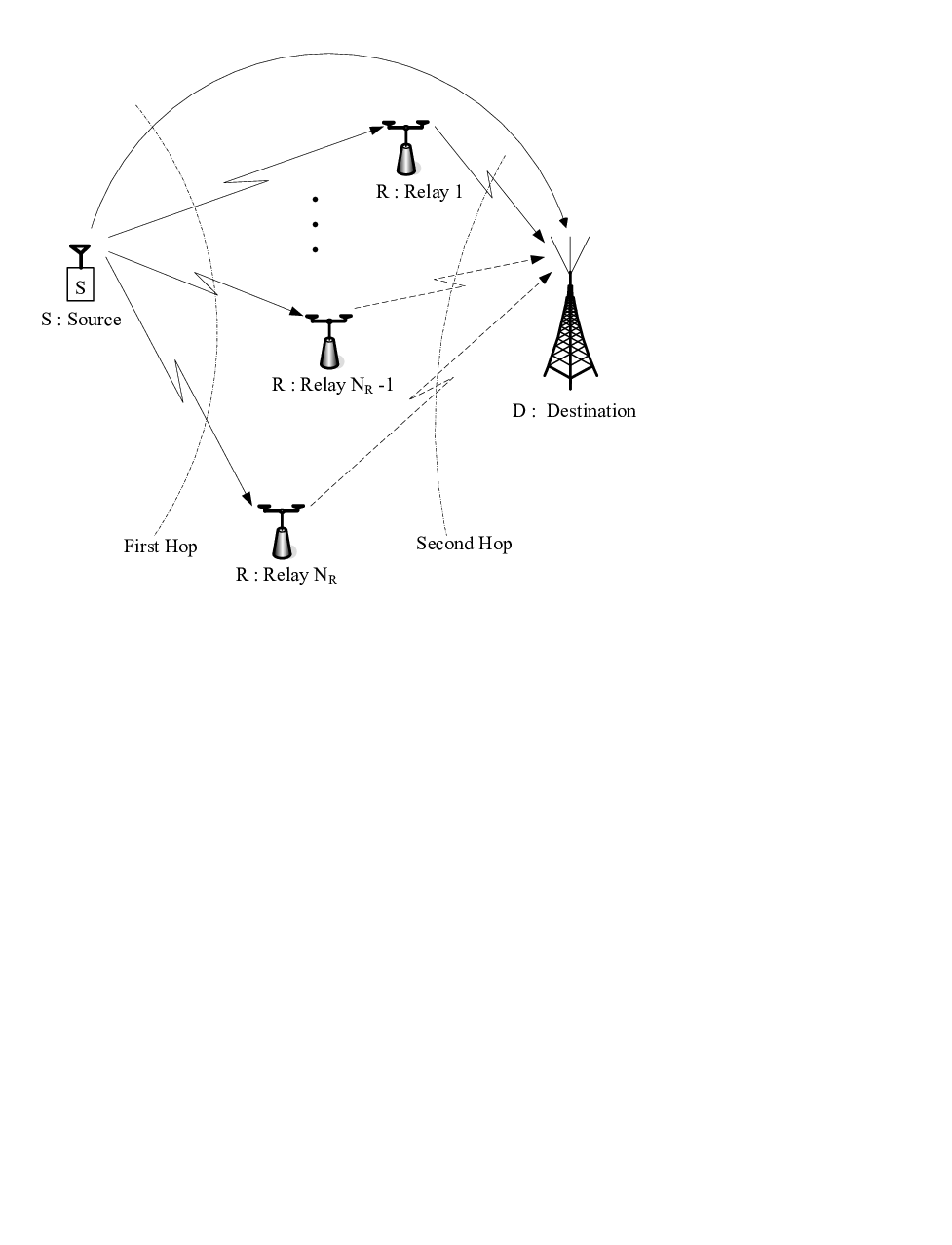
The system investigated in this paper is shown in Fig. 1. The source, destination, and relays are denoted as S, D, and R ${}_{r}\in\{1,\cdots,N_{R}\}$ , respectively. Each node is equipped with a single antenna. The best relay (chosen by some routing scheme) assists S-D communication. A block fading channel model is assumed, in which the channel does not change in the block. However, different blocks experience different channel samples that are independently and identically distributed Rayleigh random variables. $\gamma_{0}$ denotes the instantaneous SNR of the S-D link, while $\gamma_{1}$ represents the minimum SNR of the S-R and R-D links for the best relay. The Rayleigh fading model implies that $\gamma_{0}$ is an exponential random variable, and we denote its expected value by $\bar{\gamma_{0}}$ . The statistics of $\gamma_{1}$ are discussed below.

In the half-duplex two-hop protocol, S may or may not be able to communicate directly with the destination. The inability of the source to do so may be due to heavy shadowing. During the first hop, the source transmits while all the $N_{R}$ listen. During the second hop, the best relay based on a metric that depends on the S-R and R-D channels is selected to forward to the destination. The protocol assumes that the network has a mechanism to select this best relay. To that effect we state that a number of algorithms have been proposed in the literature for performing this task [6]. Thus, the objective of this paper is not to revisit path selection algorithms, but to focus on the analysis of selection relaying schemes. In our analysis, it will be assumed that the destination uses the signal received through the relay according to selection relaying, SR (the S-D path is not usable at the destination), selection cooperative relaying, SCR (the S-D link is used at the destination) and all-path selection relaying, ASR (the S-D link is among the path selection mechanism).

As mentioned above implementation issues relating to joint selection relaying schemes have been previously examined; it has been observed that selecting the best relay can be performed at a radio network controller, which comes at the expense of increased system overhead. To reduce the overhead and system complexity, [5] considered a simplified relay selection scheme based only on the R-D channel.

Refer to caption — Fig. 1: A multi-relay network with selection relaying.

III Performance Analysis

III-A Probability of Bit Error Calculations: Selection Cooperative Relaying (SCR)

The relay selection, or more accurately the path selection, is based on backward and forward channels and is performed jointly. This means that we select the relay $r^{*}$ with $\gamma=\max_{r}\min(\gamma_{s,r},\gamma_{r,d})$ , where $\gamma_{s,r}$ and $\gamma_{r,d}$ are the instantaneous SNRs of the S-R and R-D links, respectively. The signal transmitted by this selected relay is combined with the direct path signal using maximal ratio combining technique. Therefore, the combined SNR at the destination is the sum of the two SNRs. Note that the destination uses the weaker of the first and second hop of the selected relay. In terms of capacity, this weaker link constitutes the bottle-neck as far as the end-to-end performance is concerned.

Using the above notations, after maximal ratio combining, the SNR is given as $\beta=\gamma_{0}+\gamma_{1}$ . Due to the independence of $\gamma_{0}$ and $\gamma_{1}$ , the (probability density function (PDF) of $\beta$ can be obtained through the convolution of the PDFs of $\gamma_{1}$ and $\gamma_{0}$ , i.e.,

\displaystyle p(\beta)

\displaystyle=

\displaystyle\int_{0}^{\beta}p_{\gamma_{0}}(\tau)\,p_{\gamma_{1}}(\beta-\tau)\,d\tau.

(1)

As noted earlier, the selection of the best relay requires order statistics. The first step is to obtain the weaker link between the first hop and second hop of each relay node. These weak links are ordered and the one with the largest SNR is selected as the candidate relay to perform detection and forwarding to the destination. Given the PDF $f(\gamma)$ and CDF $F(\gamma)$ of the underlying Rayleigh distributed random variable, the PDF of such ordered random variables can be obtained [7] [8] as $p(\gamma)=2N_{R}\,f(\gamma)\left[1-F(\gamma))\right]\,\left[2F(\gamma)-(F(\gamma))^{2})\right]^{N_{R}-1}.$ Since $f(\gamma)=\frac{1}{\bar{\gamma}}\exp\left(\frac{-\gamma}{\bar{\gamma}}\right)$ and $F(\gamma)=1-\exp\left(\frac{-\gamma}{\bar{\gamma}}\right)$ , the PDF of $\gamma_{1}$ can be obtained as,

p(\gamma_{1})=N_{R}\,\frac{\exp(-\frac{\gamma_{1}}{\bar{\gamma_{1}}/2})}{\bar{\gamma_{1}}/2}\bigg(1-\exp\bigg(-\frac{\gamma_{1}}{\bar{\gamma_{1}}/2}\bigg)\bigg)^{N_{R}-1},

(2)

and through binomial expansion, we further can write

p(\gamma_{1})=\sum_{i=1}^{N_{R}}\left(-1\right)^{i-1}\,\left(\begin{array}[]{c}N_{R}\\ i\end{array}\right)\frac{2\,i}{\bar{\gamma_{1}}}\,\exp\left(-i\,\frac{2\gamma_{1}}{\bar{\gamma_{1}}}\right).

(3)

Using (3) and the PDF of $\gamma_{0}$ (i.e., $\frac{1}{\bar{\gamma}_{0}}\exp(-\frac{\gamma_{0}}{\bar{\gamma}_{0}})$ ), we have

	$\displaystyle p(\beta)$	$\displaystyle=$	$\displaystyle\int_{0}^{\beta}\sum_{i=1}^{N_{R}}\left(-1\right)^{i-1}\,\bigg(\begin{array}[]{c}N_{R}\\ i\end{array}\bigg)\frac{2\,i}{\bar{\gamma_{1}}\bar{\gamma_{0}}}$		(7)
		$\displaystyle\times$	$\displaystyle\exp\left(-\frac{i\,\tau}{\bar{\gamma_{1}}/2}\right)\exp\left(-\frac{\beta-\tau}{\bar{\gamma}_{0}}\right)d\tau.$		(7)

By interchanging the integral and summation, (7) can be expressed as

	$\displaystyle p(\beta)$	$\displaystyle=$	$\displaystyle\sum_{i=1}^{N_{R}}\left(-1\right)^{i-1}\,\bigg(\begin{array}[]{c}N_{R}\\ i\end{array}\bigg)\frac{2\,i}{\bar{\gamma_{1}}\bar{\gamma_{0}}}$		(11)
		$\displaystyle\times$	$\displaystyle\exp\left(-\frac{\beta}{\bar{\gamma}_{0}}\right)\int_{0}^{\beta}\exp\left(-\bigg[\frac{i\,\tau}{\bar{\gamma_{1}}/2}-\frac{\tau}{\bar{\gamma}_{0}}\bigg]\right)d\tau.$		(11)

Finally,

	$\displaystyle p(\beta)$	$\displaystyle=$	$\displaystyle\sum_{i=1}^{N_{R}}\left(-1\right)^{i-1}\,\bigg(\begin{array}[]{c}N_{R}\\ i\end{array}\bigg)\frac{2\,i}{2i\bar{\gamma_{0}}-\bar{\gamma_{1}}}$		(15)
		$\displaystyle\times$	$\displaystyle\left(\exp\left[-\frac{\beta}{\bar{\gamma}_{0}}\right]-\exp\bigg[-\frac{2\,i\,\beta}{\bar{\gamma_{1}}}\bigg]\right).$		(15)

The PDF obtained in (15) can be employed for evaluating the error performance of this relaying scheme with any modulation technique. However, we will demonstrate the evaluation with binary phase shift keying (BPSK) as follows:

$\displaystyle BER_{scr}$	$\displaystyle=$	$\displaystyle\frac{1}{2}\int_{0}^{\infty}\mbox{erfc}\left(\sqrt{\beta}\right)p(\beta)d\beta,$
	$\displaystyle=$	$\displaystyle\frac{1}{2}\int_{0}^{\infty}\mbox{erfc}\left(\sqrt{\beta}\right)\sum_{i=1}^{N_{R}}\left(-1\right)^{i-1}\,\bigg(\begin{array}[]{c}N_{R}\\ i\end{array}\bigg)$
	$\displaystyle\times$	$\displaystyle\frac{2\,i}{2i\bar{\gamma_{0}}-\bar{\gamma_{1}}}\left(\exp\left[-\frac{\beta}{\bar{\gamma}_{0}}\right]-\exp\bigg[-\frac{2\,i\,\beta}{\bar{\gamma_{1}}}\bigg]\right)\,d\beta$
	$\displaystyle=$	$\displaystyle\sum_{i=1}^{N_{R}}\left(-1\right)^{i-1}\,\bigg(\begin{array}[]{c}N_{R}\\ i\end{array}\bigg)$
	$\displaystyle\times$	$\displaystyle\frac{i}{2\,(2i\bar{\gamma_{0}}-\bar{\gamma_{1}})}\bigg[\bar{\gamma_{0}}B_{z_{0}}[1,\frac{1}{2}]-\frac{\bar{\gamma_{1}}}{2\,i}B_{z_{1}}[1,\frac{1}{2}]\bigg],$

where $z_{0}=\frac{1}{\bar{\gamma_{0}}+1}$ , $z_{1}=\frac{2\,i}{\bar{\gamma_{1}}+2\,i}$ , and $B_{x}[a,b]$ is the incomplete beta function [9].

Note that $\gamma_{1}$ ( $=\min(\gamma_{s,r^{*}},\gamma_{r^{*},d})$ ) sets the upper-bound on the end-to-end (E2E) bit error rate (BER) of this selection relaying scheme. However, the numerical examples discussed below show that the performance evaluated using these derived expressions are quite tight.

III-B Selection Relaying

In this form of relaying it is assumed that the direct path is unusable due to deep fade instances or heavy shadowing. Hence, the BER performance can be derived from expression given in () by setting $\gamma_{0}\rightarrow-\infty$ . In particular, after some manipulation, the following error rate expression can be obtained

\displaystyle BER_{sr}

\displaystyle=

\displaystyle\frac{1}{4}\sum_{i=1}^{N_{R}}\left(-1\right)^{i-1}\,\bigg(\begin{array}[]{c}N_{R}\\ i\end{array}\bigg)B_{z_{1}}[1,\frac{1}{2}],

which is a strikingly simple and compact expression.

III-C All-Path Selection Cooperating Relaying (ASR)

In this relaying scheme the destination selects one path from the $N_{R}+1$ possible paths ( the $N_{R}$ relay paths and the S-D path) for signal detection. The scheme views the S-D link as a virtual relay path (i.e., the S-R and R-D channels are the same). It then selects a path according to the previous selection scheme. The important distinction from the SCR is that the destination does not need to perform maximal ratio combining. Therefore, a system using the ASR scheme is less complex than one using SCR. Although full diversity order is obtained, the scheme is however, inferior to SCR in terms of coding (or power) gain. The antenna gain advantage of SCR over ASR is evident by comparing Figs. 2 and 4. In these two figures, the corresponding curves have the same slope, but the curves for SCR are shifted downward (i.e., in the direction of power gain or coding gain).

The ASR combiner follows almost the same principle as the traditional selection combining scheme (of collocated antennas) with the distinction that the broadcast nature of wireless channel is exploited and that the antennas (i.e., the relays) are distributed entities. The combiner in this case can be expressed as $\max\{\min\{\gamma_{S-r^{*}},\gamma_{r^{*}-D}\},\gamma_{S-D}\}$ , where $r^{*}$ is the best relay. The $\max\min$ formulation is essential to incorporate the fact that the weak link constitutes the bottle-neck.

IV Capacity and Outage Probability

System capacity and outage probability are information theoretic performance measures. Here, we demonstrate that the analyses in this paper can be extended to calculating these performance measures. The notion of capacity is valid where the channel is ergodic and there are no constraints on the decoding delay on the receiver. These conditions are hardly met in practical communication systems. The channels do behave in a manner such that there is no significant channel variability. Under such slow fading channel conditions, there is a non-zero error probability that the channel will be in a deep fade. Therefore, it is not possible to send a positive rate through the channel and yet maintain a vanishingly small error probability, which explains why in strict sense, the capacity of a slowly fading channel is zero. It is appropriate in this situation to consider outage probability. We note that outage and capacity are important communication modeling parameters, and we therefore provide expressions for evaluating them in the following discussion.

IV-1 Outage probability SCR

An outage is defined as the event where the communication channel does not support a target data rate under the SCR scheme, the outage probability is given by the following expression (see the Appendix for the derivation).

	$\displaystyle p_{out,scr}$	$\displaystyle=$	$\displaystyle\sum_{i=1}^{N_{R}}\left(-1\right)^{i-1}\,\bigg(\begin{array}[]{c}N_{R}\\ i\end{array}\bigg)\bigg(1+\frac{1}{2\,i\bar{\gamma_{0}}-\bar{\gamma_{1}}}$
		$\displaystyle\times$	$\displaystyle\bigg[\bar{\gamma_{1}}\exp\left(-\frac{2\,i\,a}{\bar{\gamma_{1}}}\right)-2i\,\bar{\gamma_{0}}\exp\left(-\frac{a}{\bar{\gamma}_{0}}\right)\bigg]\bigg),$

where $R$ is the target rate, and $a=2^{2R}-1.$

IV-2 Capacity of SCR

The ergodic channel capacity is considered. Therefore, averaging the instantaneous channel capacity over the fading distribution has operational meaning. The capacity of the SCR scheme, in bits/s/Hz, is given as

$\displaystyle\tilde{C}$	$\displaystyle=$	$\displaystyle\int_{0}^{\infty}\frac{1}{2}\log_{2}(1+\beta)p(\beta)d\beta$
	$\displaystyle=$	$\displaystyle\sum_{i=1}^{N_{R}}\left(-1\right)^{i-1}\,\bigg(\begin{array}[]{c}N_{R}\\ i\end{array}\bigg)$
	$\displaystyle\times$	$\displaystyle\left(\frac{2}{(2\,\bar{\gamma_{1}}-4\,i\bar{\gamma_{0}})\ln 2}\right)\bigg[2\,i\bar{\gamma_{0}}\exp\left(\frac{1}{\bar{\gamma_{0}}}\right)\left(E_{1}\bigg[\frac{-1}{\bar{\gamma_{0}}}\bigg]\right)$
	$\displaystyle-$	$\displaystyle\bar{\gamma_{1}}\exp\left(\frac{2\,i}{\bar{\gamma_{1}}}\right)\left(E_{1}\bigg[\frac{-2\,i}{\bar{\gamma_{1}}}\bigg]\right)\bigg]$
	$\displaystyle=$	$\displaystyle\sum_{i=1}^{N_{R}}\left(-1\right)^{i-1}\,\left(\frac{1}{(\bar{\gamma_{1}}-2\,i\bar{\gamma_{0}})\ln 2}\right)\,\bigg(\begin{array}[]{c}N_{R}\\ i\end{array}\bigg)$
	$\displaystyle\times$	$\displaystyle\bigg[-2\,i\bar{\gamma_{0}}\exp\left(\frac{1}{\bar{\gamma_{0}}}\right)E_{1}\bigg[\frac{1}{\bar{\gamma_{0}}}\bigg]+\bar{\gamma_{1}}\exp\left(\frac{2\,i}{\bar{\gamma_{1}}}\right)E_{1}\bigg[\frac{2\,i}{\bar{\gamma_{1}}}\bigg]\bigg],$

where $E_{1}[\cdot]$ is the exponential integral [9]. This capacity analysis also generalizes the single relay treatment in [10] to an arbitrary number of relays. The derivation of this result, and those below, is omitted due to space limitations.

IV-3 Outage Probability for SR

The outage probability for the SR scheme can be expressed as,

	$\displaystyle p_{out,sr}$	$\displaystyle=$	$\displaystyle\sum_{i=1}^{N_{R}}\left(-1\right)^{i-1}\left(\begin{array}[]{c}N_{R}\\ i\end{array}\right)$		(40)
		$\displaystyle\times$	$\displaystyle\,\left(1-\exp\left[-\frac{2i(2^{2\,R}-1)}{\bar{\gamma}}\right]\right).$		(40)

IV-4 Capacity for the SR

The capacity of this scheme is

	$\displaystyle\tilde{C}$	$\displaystyle=$	$\displaystyle\sum_{i=1}^{N_{R}}\left(-1\right)^{i-1}\,\left(\begin{array}[]{c}N_{R}\\ i\end{array}\right)\frac{1}{\ln 2}$		(44)
		$\displaystyle\times$	$\displaystyle\exp\left(\frac{2i}{\bar{\gamma}}\right)E_{1}\left(\frac{2\,i}{\bar{\gamma}}\right)\hskip 7.11317pt\mbox{bits/s/Hz}.$		(44)

V Numerical Examples

Figs. 2, 3 and 4 show the bit error rate of selection cooperative relaying, selection relaying and all path selection relaying schemes, respectively. BPSK modulation is used on all the links, and slow Rayleigh fading is assumed. In the SCR scheme, the S-D and S-R, and R-D links are assumed to have the same average channel gains. All receiving nodes are assumed to have the same noise statistics. From Figs. 2 and 3, simulation results indicated with symbols, match closely with the analytical ones shown as solid curves. From Fig. 2, it can be seen that a diversity order equal to $N_{R}+1$ is obtained for an $N_{R}$ relay network. This order of diversity can be calculated from the slope of the curves. The same diversity order can be calculated from Fig. 4. However, Fig. 2 presents a superior power gain advantage over Fig. 4.

The derived formulas for capacity are plotted in Fig. 5. The figure compares the capacity of the SCR and SR schemes. The capacity for SCR is shown as solid curves and SR as dotted curves. The advantage of using the direct path is also obvious from this figure, where a more than 11% increase in capacity is obtained over the capacity of the SR scheme. A general observation is that the capacity saturates quickly with the number of relays.

The analyses in this work can be applied to systems that employ coding and to systems that do not, such as in sensor networks where the node may have only detect-and-forward capability. In the latter scenario, the error rate is a valid performance criterion while in the former, where coding is used (applicable to decode-and-forward relaying) the outage or capacity is the reasonable performance measure.

VI Conclusion

Much of the recent work on selection relaying has been focused on information theoretic analyses. Bounds on high-SNR outage probability have been presented in most of these studies. In contrast to earlier works, our contributions provide error rate analyses that are reasonably accurate over a large range of SNRs, most importantly in the low/medium SNR region. It is worth noting that practical systems operate at considerably lower SNR values than the range where large SNR analysis is accurate. It is important that network designers are able to evaluate system performance with a reasonable degree of accuracy to help them make meaningful decisions regarding network design and system deployment.

This section presents the derivation of the outage probability of the selection cooperative relaying scheme.

$\displaystyle p_{out,scr}$	$\displaystyle=$	$\displaystyle\text{Pr}\,(I<R)$
	$\displaystyle=$	$\displaystyle\text{Pr}\,\big(\log\left(1+\beta\right)<2\,R\big)$
$\displaystyle p_{out,scr}$	$\displaystyle=$	$\displaystyle\int_{-\infty}^{a}\sum_{i=1}^{N_{R}}\left(-1\right)^{i-1}\,\bigg(\begin{array}[]{c}N_{R}\\ i\end{array}\bigg)$
	$\displaystyle\times$	$\displaystyle\frac{2\,i}{2i\bar{\gamma_{0}}-\bar{\gamma_{1}}}\left(\exp\left[-\frac{\beta}{\bar{\gamma}_{0}}\right]-\exp\bigg[-\frac{2\,i\,\beta}{\bar{\gamma_{1}}}\bigg]\right)d\,\beta,$

where $a=2^{2\,R}-1.$ Now by interchanging the integral and summation operations, the integration can be performed, giving the following:

	$\displaystyle=$	$\displaystyle\sum_{i=1}^{N_{R}}\left(-1\right)^{i-1}\,\bigg(\begin{array}[]{c}N_{R}\\ i\end{array}\bigg)\frac{2\,i}{2i\bar{\gamma_{0}}-\bar{\gamma_{1}}}$
	$\displaystyle\times$	$\displaystyle\int_{0}^{a}\left(\exp\left[-\frac{\beta}{\bar{\gamma}_{0}}\right]-\exp\bigg[-\frac{2\,i\,\beta}{\bar{\gamma_{1}}}\bigg]\right)d\,\beta,$
	$\displaystyle=$	$\displaystyle\sum_{i=1}^{N_{R}}\left(-1\right)^{i-1}\,\bigg(\begin{array}[]{c}N_{R}\\ i\end{array}\bigg)\frac{2\,i}{2i\bar{\gamma_{0}}-\bar{\gamma_{1}}}\bigg(\gamma_{0}-\frac{\bar{\gamma_{1}}}{2\,i}$
	$\displaystyle+$	$\displaystyle\frac{1}{2\,i}\left[\bar{\gamma_{1}}\exp\left[-\frac{2\,ia}{\bar{\gamma_{1}}}\right]-2i\bar{\gamma_{0}}\exp\left[\frac{-a}{\bar{\gamma_{0}}}\right]\right]\bigg).$
Finally,			(55)
$\displaystyle p_{out,SCR}$	$\displaystyle=$	$\displaystyle\sum_{i=1}^{N_{R}}\left(-1\right)^{i-1}\,\bigg(\begin{array}[]{c}N_{R}\\ i\end{array}\bigg)\bigg(1$
	$\displaystyle+$	$\displaystyle\frac{1}{2\,i\bar{\gamma_{0}}-\bar{\gamma_{1}}}\left[\bar{\gamma_{1}}\exp\left(-\frac{2\,ia}{\bar{\gamma_{1}}}\right)-2i\bar{\gamma_{0}}\exp\left(\frac{-a}{\bar{\gamma_{0}}}\right)\right]\bigg).$

This completes the derivation. The outage performance expression for the selection relaying scheme (without the direct path) can be derived in a similar way through the PDF in (3). However, it can also be obtained from (). The expression is given as

	$\displaystyle p_{out,sr}$	$\displaystyle=$	$\displaystyle\int_{-\infty}^{2^{2R}-1}p(\gamma)\,d\gamma$
		$\displaystyle=$	$\displaystyle\sum_{i=1}^{N_{R}}\left(-1\right)^{i-1}\,\bigg(\begin{array}[]{c}N_{R}\\ i\end{array}\bigg)\left(1-\exp\left[-\frac{2\,ia}{\bar{\gamma}}\right]\right).$

References

[1] J. Laneman, D. Tse, and G. Wornell, “Cooperative diversity in wireless networks: efficient protocols and outage behavior,” IEEE Trans. Inform. Theory, 50(11), pp. 3062-3080, Dec. 2004.
[2] A. Sendonaris, E. Erkip, and B. Aazhang, “User cooperation diversity - Part I: system description,” IEEE Trans. Commun., 51(11), pp. 1927-1938, Nov. 2003.
[3] Y. Hua, Y. Mei, and Y. Chang, “Parallel wireless mobile relays with space-time modulations,” Proc. IEEE Workshop on Statistical Signal Processing, pp. 375 - 378, St. Louis, MO, USA, Sept. 2003.
[4] F. Atay Onat, A. Adinoyi, Y. Fan, H. Yanikomeroglu, and J. Thompson, “Threshold selection for SNR-based selective digital relaying in cooperative wireless networks,” to appear in IEEE Transactions on Wireless Communications, 2008.
[5] E. Beres and R. Adve, “Selection cooperation in multi-source cooperative networks,” IEEE Trans. Commun., 7(1), pp. 118-127, Jan. 2008.
[6] A. Bletsas, A. Khisti, D. Reed, and A. Lippman, “A simple cooperative diversity method based on network path selection,” IEEE J. Selected Areas Commun., 24(3), pp. 659-66, Mar. 2006.
[7] N. Balakrishnan and A. C. Cohen, Order Statistics and Inference: Estimation Methods, Academic Press, New York, 1991.
[8] L. Dai, B. Gui, and L. J. Cimini, “Selective Relaying in OFDM Multihop cooperative networks,” Proc. IEEE Wireless Commun. & Networking Conf. (WCNC), pp. 964 - 969, HongKong, China, Mar. 2007.
[9] I. Gradshteyn and I. Ryzhik, Table of Integrals, Series, and Products, Academic Press, San Diego, 1994.
[10] M. Hasna, “On the capacity of cooperative diversity systems with adaptive modulation,” Proc. Second IFIP International Conference on Wireless and Optical Communications Networks pp. 432 - 436, Dubai, UAE, Mar. 2005.