Clustering of luminous red galaxies I:
large scale redshift space distortions
Abstract
This is the first paper of a series where we study the clustering of LRG galaxies in the latest spectroscopic SDSS data release, DR6, which has 75000 LRG galaxies covering over 1 at . Here we focus on modeling redshift space distortions in , the 2-point correlation in separate line-of-sight and perpendicular directions, on large scales. We use large mock simulations to study the validity of models and errors. We show that errors in the data are dominated by a shot-noise term that is larger than the Poisson error commonly used. We first use the normalized quadrupole for the whole sample (mean z=0.34) to estimate , where is the linear velocity growth factor and is the linear bias parameter that relates galaxy to matter fluctuations on large scales. We next use the full plane to find (h=0.72) and the biased amplitude . For standard gravity, we can combine these measurements to break degeneracies and find , and . We present constraints for modified theories of gravity and find that standard gravity is consistent with data as long as . We also calculate the cross-correlation with WMAP5 and show how both methods to measure the growth history are complementary to constrain non-standard models of gravity. Finally, we show results for different redshift slices, including a prominent BAO peak in the monopole at different redshifts. The data on large scales is shown to be in remarkable agreement with predictions and shows a characteristic large region of negative correlation in the line of sight, a BAO ring and a prominent radial BAO peak. The significance of this is presented in paper IV of this series. We include a study of possible systematic effects in our analysis to find that these results are quite robust.
1 Introduction
Galaxy clustering allows the study of different physical phenomena at each scale. On large scales density fluctuations are small and can be modeled by linear theory to constrain cosmological parameters. We need large surveys with galaxy positions to do this.
The measured redshift distance of a galaxy differs from the true radial distance by its peculiar velocity along the line-of-sight . These displacements lead to redshift distortions, with two important contributions. The first, on large scale fluctuations, is caused by coherent bulk motion. We see walls denser and voids bigger and emptier, with a squashing effect in the 2-point correlation function along the line-of-sight, known as the Kaiser effect [Kaiser ¡1987¿]. At small scales, random velocities inside clusters and groups of galaxies produce a radial stretching pointed at the observer, known as fingers of God (FOG) [Jackson ¡1972¿].
Although such distortions complicate the interpretation of redshift maps as positional maps, they have the advantage of bearing unique information about the dynamics of galaxies. In particular, the amplitude of the quadrupole redshift distortion on large scales yields a measure of the linear redshift distortion parameter , which is related to the matter density, and gives direct information on the growth of the newtonian gravitational potential and bias , which describes how the number density of galaxies traces matter density (see Eq.(3)). We will also show how one can use the anisotropic redshift distortions, broken into line of sight and perpendicular directions, to find separate measurements for and .
In this work we use the most recent luminous red galaxies (LRGs) from the spectroscopic SDSS public data release DR6 [Adelman-McCarthy et al ¡2006¿], and perform studies of linear bias on large scales to obtain cosmological parameters. As we will see, we can break the degeneracy between and present in the correlation function thanks to redshift distortions anisotropies, and look at the growth history and possible modifications of the gravity (see Linder 2005, Guzzo et al 2008 and the recent Yamamoto et al 2008).
A dark energy dominated universe causes gravitational potentials to evolve, changing the energy of CMB photons passing through them. This is the so called Integrated Sachs-Wolf (ISW) effect. Here, we have also cross-correlated LRGs with WMAP [Hinshaw et al ¡2008¿] in order to investigate this ISW effect, reproducing a high signal as seen in recent studies (see Gaztanaga etal 2006, Giannantonio et al 2008), as compared to current model. In this way, we can also break the degeneracy and study the growth history using the cross-correlation between temperature of CMB and galaxies , which give independent constraints on bias and compared with those obtained from redshift space distortions.
The same LRGs (but with reduced area) have been studied from different points of view. Tegmark et al (2006) have done an analysis of the power spectrum at large scales to obtain cosmological parameters. Zehavi et al (2005) study LRGs at intermediate scales (0.3 to 40Mpc/h), where they calculate the projected correlation function, the monopole and real-space correlation function to study mainly the linear high bias, the non-linear bias and the differences between luminosities, remarking that there are differences from a power law for scales smaller than 1Mpc/h.
While we were working on our results, a very interesting paper by Okumura et al (2008) showed the first application of the anisotropy in the 2-point correlation function including the baryonic features, to obtain constraints on cosmological parameters. They use the DR3 spectroscopic sample of LRGs to calculate the 2-point correlation function with a different definition of what parallel and perpendicular directions mean (the line of sight is defined in their paper as the direction toward the galaxy 1, Matsubara 2004). They fit for large scales using the linear Kaiser model, from 40Mpc/h to 200Mpc/h, excluding the FOG zone. They point out that a direct measurement of the growth function can be obtained from the distortion to the clustering signal caused by bulk flows (Kaiser anisotropy). Although constraints are weak by now, the fitting of all the anisotropic 2-point correlation function, including the baryonic feature, would enable us to divide the effect of redshift distortions into dynamical and geometrical components. The anisotropy due to geometric distortion contributes to a better estimation of the equation of state of the dark energy. Here we try to obtain new constraints, encouraged by the fact that DR6 has doubled the volume of DR3.
There has already been significant progress in this direction using LRG. Eisenstein et al (2005) detected the baryon acoustic peak in the 2-point correlation function using LRGs. Hütsi (2006 a,b) use LRGs to constrain cosmological parameters in the power spectrum, including the baryonic peak. Percival et al (2007) have analyzed also the LRGs using both 2dF and SDSS. Padmanabhan et al (2007) used the photometric catalog to work with a bigger set of LRGs with photometric redshifts, obtaining also cosmological constraints, the same as Blake et al (2007), which work with the MegaZ-LRG, a photometric-redshift catalog of luminous red galaxies based on the imaging data of the SDSS DR4.
This is the first and main paper of a series on clustering of LRG. Here we will focus on redshift space distortions in on larges scales. In Paper II [Cabré and Gaztañaga ¡2008¿] we will look at small scales in and address the issue of the FOG. In Paper III [Gaztañaga et al ¡2008¿] we look at the 3-point function and in Paper IV [Gaztañaga et al ¡2008¿] we will focus on the significance of the BAO detections. In this first paper we present the basis for the error analysis and the study of systematics effects that will be used in the rest of the series.
The paper is organized as follows. Section II gives a summary of the theory involved in redshift space distortions, the model used for the 2-point correlation function in separate line of sight and perpendicular directions, and the different multipoles. Section III presents an accurate description of the data selected to work with, LRG galaxies. Section IV is the main part of this paper, where we explain the analysis done and our main results. We use the distortions in redshift space to obtain the distortion parameter , , and modifications to gravity. We also look at the ISW effects for this LRG data, and explore the differences between redshift slices. As usual, we end with discussion and future work in section V. The Appendix A is devoted to present the mock simulations that we use to validate the errors used, Monte Carlo, jackknife and a new theoretical approach. In this section, we also validate the methods used to obtain constraints (section IV) in real data with our mocks. In the Appendix B we present a study of possible systematic effects.
2 Theory
Kaiser (1987) pointed out that, in the large-scale linear regime, and in the plane-parallel approximation (where galaxies are taken to be sufficiently far away from the observer that the displacements induced by peculiar velocities are effectively parallel), the distortion caused by coherent infall velocities takes a particularly simple form in Fourier space:
| (1) |
where is the power spectrum of density fluctuations , is the cosine of the angle between and the line-of-sight, the subscript indicates redshift space, and is proportional to the velocity growth rate in linear theory.
If the galaxy overdensity is linearly biased by a factor relative to the underlying matter density of the Universe,
| (2) |
then the observed value of is
| (3) |
where is the linear density growth factor and the velocity growth rate, which we can write as:
| (4) |
where is the gravitational growth index [Linder ¡2005¿], is the matter density at a redshift z where ,
| (5) |
where is the matter density at z=0 (which is often just called ) and
| (6) |
where is dark energy equation of state parameter.
By construction [Linder ¡2005¿], the growth index formalism separates out two physical effects on the growth of structure: involves the expansion history and focuses on the gravity theory. The value corresponds to standard gravity, while is different for modified gravity, for example in the braneworld cosmology [Linder ¡2005¿]. The linear density growth factor can be found using Eq.(3):
| (7) |
2.1 Modelling
Hamilton (1992) translated Kaiser’s results into real space,
| (8) |
where is the separation along the line-of-sight (LOS) and is the separation in the plane of the sky ,the absolute distance of separation is , is the cosine of the angle between and the line-of-sight and are Legendre polynomials.
We use these relations to create a model . In this paper, which analyzes large scales, we will use a linear real space correlation function as input [Eisenstein and Hu ¡1998¿].11 1 We have also tested the inclusion of the effect of non-linear growth (with the halofit model) and non-linear bias. We find no changes on our fit to large scales, as expected. Then we convolve it with the distribution function of random pairwise velocities, , to give the final model [Peebles ¡1980¿]:
| (14) |
where we divide peculiar velocities by to translate to comoving distances, since velocities are defined in physical coordinates.
We represent the random motions by an exponential form,
| (15) |
where is the pairwise peculiar velocity dispersion. An exponential form for the random motions has been found to fit the observed data better than other functional forms [Ratcliffe et al ¡1998¿, Landy ¡2002¿]. We have also checked this relation with our simulations, which will be described later on.
Matsubara (2004) and Scoccimarro (2004) have presented different models for the 2-point correlation function in redshift space. Tinker et al (2006) and Tinker (2007) model redshift space distortions in the context of halo occupation distribution model (HOD). These models are complementary to the one studied here. In most situations the differences are small and we will show that our modeling gives good agreement with simulations and real data.
2.2 Multipoles of
We can define the multipoles of as
| (16) |
where is cosine of the angle to the line-of-sight .
The normalized quadrupole is defined as [Hamilton ¡1992¿]
| (17) |
Linear bias in Eq.(2) cancels in the quadrupole, and is only very slightly dependent on the shape of the correlation function, such as changes on large scales due to varying or scale dependent non-linear bias for small scales.
In the Kaiser approximation, ie at large scales, the quadrupole is directly related to :
| (18) |
The validity of this approximation is studied using simulations in section A. At small scales, the quadrupole depends strongly on the random pairwise velocities, represented by , but it does not depend much on non-linear bias, as we will show.
2.3 The real-space correlation function
We can estimate the real-space correlation function by calculating the projected correlation function, , integrating the redshift distorted along the line-of-sight .
| (19) |
We would like , however, with real data, we can not integrate until infinity. Here we will use . The result does not change when we change the upper limit of the integral for and large in the data.
Davis and Peebles (1983) show that is directly related to the real-space correlation function.
| (20) |
It is possible to estimate by directly inverting [Saunders et al ¡1992¿]
| (21) |
Assuming a step function for in bins centered on , and interpolating between values,
| (22) |
for .
We take the redshift space anisotropic model in Eq.(14), with a fixed and , and we use Eq.(19) to obtain the projected correlation function as if it was data. We use different values to fix the upper limit in the integral: 60Mpc/h, 80Mpc/h, 100Mpc/h and 200Mpc/h (color lines in top panel of Fig.1), and compare the ”true” result obtained from Eq.(20) (solid line in top panel of Fig.1). As we increase we approach the true result, but we can not integrate until 200Mpc/h in real data because, as will be shown in the following sections, data is quite noisy for . The implication of these results is that we will not be able to recover the true values of from . But we can use this method at smaller scales (see Paper II).
In the bottom panel of Fig.1 we see the real-space correlation
function recovered from the previously calculated projected correlation function
with different , Eq.(21). We obtain a good estimation of
below 30Mpc/h, where we will study the non-linear bias
(see Paper II).
This analysis has been done for different values of and and
we find very similar conclusions. For illustration, we have shown in our plots
the values that are more in concordance with real LRG SDSS data.


Once we recover the real-space correlation function, we can also estimate the ratio of the redshift-space correlation function, , to the real-space correlation function, , which gives an estimate of the redshift distortion parameter, , on large scales:
| (23) |
As we have shown in Fig.(1), will be in general slightly overestimated at large scales when we estimate it from the projected correlation function , so the expression will in general be slightly lower than expected on large scales.
3 The Data

The luminous red galaxies (LRGs) are selected by color and magnitude to obtain intrinsically red galaxies in Sloan Digital Sky Survey (SDSS). See Eisenstein et al (2001) or http://www.sdss.org for a complete description of the color cuts. In this paper, we work with the last public catalog, DR6, which covers a solid angle of in the sky. These galaxies trace a big volume, around , which make them perfect to study large scale clustering. LRGs are supposed to be red old elliptical galaxies, which are usually passive galaxies, with relatively low star formation rate.
They have steeper slopes in the correlation function than the rest of galaxies,since in some cases, there is more than one LRG per halo. They trace a big volume, so they represent good candidates to use as dark matter clustering tracers.
LRG’s are targeted in the photometric catalog, via cuts in the (g-r, r-i, r) color-color-magnitude cube. Note that all colors are measured using model magnitudes, and all quantities are corrected for Galactic extinction following Schlegel et al (1998). The galaxy model colors are rotated first to a basis that is aligned with the galaxy locus in the (g-r, r-i) plane according to:
= (r-i) - (g-r)/4 - 0.18
= 0.7(g-r) + 1.2[(r-i) - 0.18]
Because the 4000 Angstrom break moves from the g band to the r band
at a redshift z 0.4, two separate sets of selection
criteria are needed to target LRGs below and above that redshift:
Cut I for z 0.4
rPetro 13.1 + / 0.3
rPetro 19.2
0.2
24.2 mag
- 0.3
Cut II for z 0.4
19.5
0.45 - (g-r)/6
g-r 1.30 + 0.25(r-i)
24.2 mag
- 0.5
where is the mean surface brightness within the radii containing 50% of Petrosian flux.
Cut I selection results in an approximately volume-limited LRG sample to z=0.38, with additional galaxies to z 0.45. Cut II selection adds yet more luminous red galaxies to z 0.55. The two cuts together result in about 12 LRG targets per that are not already in the main galaxy sample (about 10 in Cut I, 2 in Cut II). The radial distribution and magnitude-redshift diagrams are plotted in Fig.32 and Fig.43.
We k-correct the r magnitude using the Blanton program ’kcorrect’ 22 2 http://cosmo.nyu.edu/blanton/kcorrect/kcorrect_help.html. We need to k-correct the magnitudes in order to obtain the absolute magnitudes and eliminate the brightest and dimmest galaxies. We have seen that the previous cuts limit the intrinsic luminosity to a range , and we only eliminate from the catalog some few galaxies that lay out of the limits. Once we have eliminated these extreme galaxies, we still do not have a volume limited sample at high redshift but we will account for this using a random catalog with identical selection function.
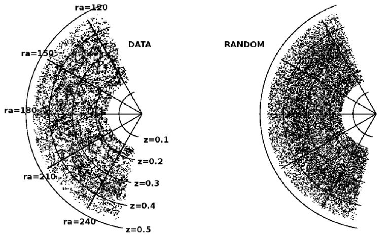
We show the comoving density in Fig.2 once we have removed the brightest and dimmest galaxies, and in Fig.3 we show the redshift space distribution in a slice of dec = 32-40 deg. We compare it with the same slice of random points. We see clear evidence of clustering in the data.
We have masked the catalog using at the first step the photometric DR6 mask, based on the number of galaxies per pixel. In previous works [Cabré et al ¡2006¿] we showed that the mask that we obtain statistically by dropping out the pixels with small number of galaxies (see §B3 for details) gives identical correlation function that the one obtained when extracting the polygons masked by the SDSS team. After that, we compare our masked catalog to the LRG spectroscopic catalog, and we extract the galaxies that lay outside from the “good” plates. Fig.40 illustrates the result.
The mask could imprint spurious effects at very small scales. But we are not focused in such small scales, because fiber collisions in the redshift catalog are limiting our analysis. This is for distances less than 55arc sec, ie less than 0.3Mpc/h at the mean redshift of LRG data, z=0.34 (see Fig.17 below). We obtain 75,000 galaxies for the final catalog, from z=0.15 to z=0.47, ie over one cubic Gigaparsec ().
4 Results


In this section we analyze the LRGs from SDSS DR6. First, we have used credible simulations to study the errors carefully as well as the methods that we use here (see Appendix A for an extensive description).
Here we define the parameters that we assume during all this work, which are motivated by recent results of WMAP, SNIa and previous LSS analysis 33 3 see http://lambda.gsfc.nasa.gov/product/map/dr3/parameters.cfm: , , . We will use the power spectrum analytical form for dark matter by Eisenstein and Hu (1998), and the non-linear fit to halo theory by Smith et al (2003). For part of our analysis we have followed the method explained in Hawkins et al (2003), an extensive analysis of redshift distortions in the 2dF catalog.
To estimate the correlation , we use the estimator of Landy and Szalay (1993) as in Eq.(32), with a random catalog times denser than the SDSS catalog. The random catalog has the same redshift (radial) distribution as the data, but smoothed with a bin to avoid the elimination of intrinsic correlations in the data. Randoms also have the same mask. We count the pairs in bins of separation along the line-of-sight (LOS), , and across the sky, . The LOS distance is just the difference between the radial comoving distances in the pair. The perpendicular distance between the two particles corresponds approximately to the mean redshift. It is exactly defined here as , where is the distance between the particles. We use the wide-angle approximation, as if we had the catalog at an infinite distance, which is accurate until the angle that separates the galaxy pair in the sky is larger than 15 degrees for the quadrupole and about 10 degress for the [Szapudi ¡2004¿, Matsubara ¡2000¿]. This later restriction corresponds to scales for our mean catalog.
In Fig.4 we can see our estimation for LRG DR6 catalog and for MICE simulations (with a linear bias b=2 to see similarities visually). Here we can clearly see the FOG at small as we have increased the pixel resolution when we approach the central part of the image (pixel size varies from 0.2 Mpc/h in the center to 10 Mpc/h at large scales). As expected, simulations have less noise because we have done the mean over 216 mocks. Moreover, the distortion parameter is higher in the simulations than in data because of the high bias of LRG, as can be seen in the shape of the 2-point correlation function, which gets more flattened as increases. We see clearly the baryonic peak, as a ring in the correlation function . This feature is studied in detail in Paper IV of this series. In next sections we will analyze all the information hidden in this figure, using the analytical form of the error (see §A.2).
4.1 Quadrupole and estimation


We use the normalized quadrupole Q(s) to obtain (extensive explanation can be found in §A.5). But first, we can measure using the asymptotic large scale value in the quadrupole where there is no dependence on (see Eq.(18)). We find in the range ; for and for . In Fig. 5 we see the quadrupole with jackknife errors at large scales and the error obtained in , translated to the quadrupole as a band of red dots.
The quadrupole only depends strongly on and . It does not depend on linear bias because it cancels out in the ratio, and it does not depend much on the shape of the 2-point correlation function ( and other parameters) or in the non-linear bias for small scales. We have tried to fit and using all the scales in the quadrupole, fixing to 0.25 (which in our model means fixing the shape of the real-space correlation function) and we use a power law form for the non-linear bias. When we change the shape of the in the model (that is for large scales and non-linear bias for small scales) , we obtain the same contours for , so we arrive to the conclusion that the normalized quadrupole is a good estimator to find separately from the other parameters, which are degenerate with them in the plane.
We can obtain better errors in by doing a joint fit with and using smaller scales, as we do with simulations in Appendix A. We will fit the quadrupole above 5Mpc, because this seems a reliable scale according to simulations and results do not change much when using a cut on larger scales. Below this minimum scale, starts increasing, and even when this has only a small effect in the quadrupole at larger scales, it can bias the value of when doing a fit to all scales.
In Fig.6 we show the fit as contours in the plane (top panel) and the best fit to Q(s) for the mean slice (bottom panel). We have fitted for different slices in redshift. First, we divide the catalog in 3 redshift slices: z=0.15-0.3, z=0.3-0.4, z=0.4-0.47. And then, we divide it in 2 redshift slices: z=0.15-0.34, z=0.34-0.47. The fitted values and are similar in all the redshift slices (see table 1). This is a bit surprising because we expect to increase slightly with , for this redshift range. The similarity in the value of the distortion parameter means that the bias must also increase as a function of redshift, roughly in the same way as so that the effect cancels out (see Eq.(3)). This is not totally surprising, because we expect bias to scale with redshift as , the inverse of the growth factor, , which is proportional to , in order to have stable clustering, ie constant along redshift (Peebles 1980).
| Sample | (km/s) | |
| z=0.15-0.47 | 0.310-0.375 | 365-415 |
| z=0.15-0.34 | 0.280-0.365 | 320-410 |
| z=0.34-0.47 | 0.305-0.405 | 345-420 |
| z=0.15-0.30 | 0.280-0.395 | 305-435 |
| z=0.30-0.40 | 0.285-0.365 | 335-390 |
| z=0.40-0.47 | 0.270-0.415 | 305-420 |
4.2 Fitting

We have calculated the real-space correlation function integrating through the LOS direction (Eq.(21)). This method is complementary to the estimation from angular correlation [Baugh ¡1996¿]. In Fig.7 we compare (in blue) with the monopole (orange) for the main slice in redshift. The difference at large scales (r 5Mpc/h) is a constant value, at least until where we can trust the recovered . Note that, although we expect the recovered to be systematically biased at large scales (eg see Fig1), we can still see the baryonic peak at , in real space! So this is a strong feature in the LRG data.
The large differences at small scales are due to random velocities, which we will study in more detail in Paper II of this series.

In Fig.8 we show the ratio and we have overplotted the constant value in the Kaiser approximation (Eq.(23)), using the value of obtained with Q(s), ie . This gives a good fit but note how it would be quite difficult to estimate from this ratio given how noisy the data becomes when we reach an asymptotic constant value in .
4.3 Fitting large scales in
We obtain from the anisotropic redshift-space correlation function using the full covariance matrix from the MICE group mocks (more details in §A.5). Here refers to the factor . The growth factor , which is a function of , has been included in the model of . We do not find any difference when fitting with models with non-linear bias (as used in Paper-II) or linear bias. This is because we restrict our analysis to scales from 20Mpc/h to 60Mpc/h and for angles above 30-40 deg away from the line-of-sight in the plane.

In Fig.9 we show constraints on for the slice z=0.15-0.34. We have used the obtained with the quadrupole Q(s) fit to marginalize the space of parameters in the fit, although this only makes a slight difference. The values of and are strongly degenerate in the range where we fit large scales, but is not strongly degenerate with the other parameters, since we are located away from the fingers of God, where we have the strongest effect of . When we marginalize, we assume that the likelihood scales as .
We have done the same analysis for different redshift slices. We have summarized the results in table 2 where we have annotated the marginalized 1- errors for the amplitude Amp= and for . Note that we use a fixed value of to model the shape the linear power spectrum.
| Sample | ||||
| z=0.15-0.47 | 1.47-1.65 | 0.225-0.265 | 1.73-1.94 | 0.54-0.73 |
| z=0.15-0.34 | 1.45-1.62 | 0.230-0.275 | 1.71-1.91 | 0.48-0.70 |
| z=0.34-0.47 | 1.55-1.82 | 0.215-0.285 | 1.82-2.14 | 0.56-0.87 |
| z=0.15-0.30 | 1.45-1.80 | 0.240-0.320 | 1.71-2.11 | 0.48-0.83 |
| z=0.30-0.40 | 1.42-1.60 | 0.210-0.260 | 1.67-1.88 | 0.48-0.69 |
| z=0.40-0.47 | 1.60-2.00 | 0.195-0.305 | 1.88-2.35 | 0.51-0.98 |
If we try to fit to even larger scales, we always obtain a slightly biased low compared to the one we obtain in the scales before the acoustic peak, probably because wide angle effects that we are not taking into account in the modelization (see §B.5) but possibly also because non-linear effects on the BAO peak and large sampling errors. We have also seen this effect in the simulations, where we have checked that the best region to obtain parameters is at intermediate to large scales, where we do our fit.
Note how the best fit values of seem to change from sample to sample. This could be due to bias, which is both a function of and luminosity. The values of agree within for 2 degrees of freedom (dotted lines).
In Fig.10 we have plotted the with the best model overplotted in solid lines. We can see how this simple Kaiser model can explain most features in the observations. There is a very good agreement on the region of negative correlation (in blue) which is a very good tracer of and (see Paper IV). All these features are very significant given the errors and their coherence over large regions. We can clearly see the FOG at small as we have increased the pixel resolution when we approach the central part of the image (pixel size varies from 0.2 Mpc/h in the center to 5 Mpc/h at large scales). The baryonic peak can also be seen in both the data and in the models. The significance of this is studied in detail in Paper IV, while the smaller scales and the prominent fingers of God are presented in Paper II [Cabré and Gaztañaga ¡2008¿].

4.4 The value of
We first try to obtain a fit to the parameter , which we can separate from the bias thanks to redshift distortions, following Eq.(3) and Eq.(4). We use our previous estimation of from large scales (ie Table 2) and the value of from Q(s) (ie in Table 1), using , for standard gravity. As , we obtain from:
| (24) |
where is given in Eq.(5).
We also assume a flat universe (WMAP results motivated) with a constant dark
energy equation of state characterized by (ie as in
the cosmological constant model).


In the top panel of Fig.11 we show , marginalized over , and in each sample. We also show results using a fixed value of for all samples (bottom panel). There seems to be a lower detection for the middle slice of z=0.3-0.4, but it is consistent with the others at level. In the same figures we also show the estimated bias from the amplitude and the values . For a fixed , the linear bias seems higher as we move to higher redshifts, and it is consistent with previous results found also with LRG [Zehavi et al ¡2005¿, Tegmark et al ¡2006¿, Okumura et al ¡2008¿]. Note that the luminosity of the galaxies also increases with redshift and this is probably the main reason for the increase in (more luminous galaxies trace higher density peaks and therefore are more biased). There is one exception to this tendency in slice . The values of for the best fit are shown in Table 2, were we can see how is lower for . This is due to the LRG selection explained in §3, which includes a population of less luminous galaxies at (see Fig.43) resulting in a lower bias.
Once we know the bias we can use the values of to estimate the linear velocity growth function for each slice, which are also shown in Table 2.
4.5 Modified gravity
We can also use redshift distortions to constrain modified gravity. For standard gravity, the linear theory growth factor, , depends purely on the expansion history , , . Any discrepancy found between the observed growth factor and predictions based on the expansion history can be used to test the gravity.
The idea of using the growth of structure to test gravity has a long history and dates back to Brans-Dicke (BD) model (see Brans 2005 for a historical review). More recently, after cosmic acceleration, the BD and variations have been revisited to explore structure formation outside general relativity [Gaztañaga and Lobo ¡2001¿, Lue et al ¡2004¿, Lue et al ¡2004¿, Acquaviva et al ¡2008¿]. Zhang et al (2007) propose a test to discriminate between different models for gravity on cosmological scales based on lensing. Nesseris and Perivolaropoulos (2008) have compiled a data set of various observations of the growth rate at different redshifts, obtained through redshift distortions or indirectly through the rms mass fluctuation inferred from . These data points are used to constrain and parametrize the linear perturbation growth rate . Wang (2007) does a prediction of the characteristics that a survey must accomplish to be able to rule out the DGP gravity model (an extra-dimensional modification of gravity), where the idea is to calculate H(z) from the baryon acoustic peak and f(z) from redshift distortions. Guzzo et al (2008) test the nature of cosmic acceleration using galaxy redshift distortions at z=0.8, obtaining , but errors are still too high to distinguish between different theories. Acquaviva et al (2008) have recently done a new compilation of results. See Bertschinger and Zukin (2008) for a theoretical approach to modified gravity.
If we fix a value for , which can also be known from other observations, we can assume that the changes in the amplitude with redshift could be explained by changes in the growth factor due to a different law of gravity at cosmological scales [Linder ¡2005¿]. This can be represented by the growth index . Both and the growth factor changes with . We have plotted in Fig.12 how and change with for z=0.34 (mean redshift in LRG) and . The measured amplitude on large scales depends linearly on the product . If we now fix we can have an estimation of as well as our separate estimation of , from the quadrupole. We therefore can use this combined data to produce an estimate of .

We have assumed that the observations can be explained by varying , for a fixed dark energy equation of state . This is a good approximation because only depends slightly on [Linder ¡2007¿]. We show in Fig.13 our estimation of errors for the growth index once we fix =0.7, 0.8, 0.9 and marginalized over , and . As shown in Fig.12, the product , at a given redshift, decreases with . If we change the value to higher values, the factor obtained from observations will be lower, and this needs to be compensated by reducing , thus increasing . In next section (§4.6) we will show how the argument goes in the opposite way when we work with ISW effect. At and for all the redshift slices, is consistent with a standard gravity, except for where we need for the last slice, favoring a clearly higher than 0.7, which is in agreement with recent observations.


Following this argument, we can calculate which is the range of that is consistent with standard gravity, . We find at 1-. In the modified gravity DGP model, needs to be higher since is also higher (). We could say that DGP model is inconsistent with data if . These results are in agreement with the recent study of Yamamoto et al (2008), which appeared as we were writing this paper.
4.6 Angular correlation and cross-correlation with WMAP
We can also learn about the growth of fluctuations using the ISW effect. This method is independent to the one explained before with redshift distortions (see Cabré et al 2007 and references therein for an explanation of the ISW effect in the context of SDSS galaxies). In this section we explore the angular correlation function and also the ISW effect through the cross-correlation between galaxies and fluctuations of temperature in WMAP. Fig.14 shows the results for and at the redshift slice z=0.15-0.34. This is the same data that we have used before, but we now look at angular clustering. The angular auto-correlation function GG scales as:
| (25) |
while the cross-correlation function between galaxies and CMB temperature fluctuations is proportional to
| (26) |
where
| (27) |
and is the galaxy selection function. Both and are proportional to because this factor comes from the normalization of the power spectrum, but is proportional to while is proportional to (from the clustering of galaxies) and (from the evolution of gravitational potentials). Thus, this allows for a separate estimation of these quantities [Fosalba et al ¡2003¿].
We find that the measured signal of in Fig.14 is higher than expected, a clear tendency that has been seen before (see Gaztanaga etal 2006, Giannantonio et al 2008 for a compilation of ISW observations). The high signal could be due to: sampling variance, higher , lower , non-linear effects, bias between matter and galaxies different from the one obtained from galaxies-galaxies, non-linear bias, different form of dark energy as (see Cabré et al 2006 for some hints in this direction), modified gravity at cosmological scales, or non-linear magnification (linear magnification is not expected to affect ISW at low redshifts, Loverde et al 2007).
The signal to noise is not very high so we can not obtain tight constraints, but we can explore what could be creating this high signal. We study two reasons here: a change in or a change in the growth index . We have also studied these two parameters in the section above of redshift distortions and we want to see if results are compatible.
We can break the degeneracy between and in the auto-correlation function , which is proportional to , by combining the result with , which goes as . We will assume that is constant through all the redshift slice, to be consistent with the previous section of redshift distortions.
We fix the shape ( and flat universe) of and use the amplitude to find the factor . This should be equal to the amplitude that we found in previous sections, when analyzing 3D redshift distortions, since we are working with the same LRG galaxy samples. We find that this is the case: both measurements of the amplitude are consistent within the errors. There is an extra power at large scales ( degrees) as in the 3D case that can be due to sampling variance. This is explained with more detail in §B. We next fix the dark energy equation of state parameter to and to standard gravity. We now try to explain the observed amplitude of by just changing . We therefore break the degeneracy of with bias in a way that is completely independent from the one used in the previous section, based on 3D redshift distortions. In bottom panel of Fig.14, we have compared to the best model (in red) which corresponds to . This value is quite high but the errors in are also large, so that at 1- (or for some of the redshift slices), the values of are consistent with our previous estimation.
We next see how we could explain the observed high ISW signal if it is due to a modification of gravity. We fix and vary . We assume that changes only slightly with and that almost all the variation with in ISW comes from the factor . Both and grow with , so that also grows with (see Fig.12). Thus if we fix to a low value we need larger values of from the ISW effect, but lower values of from redshift space distortions. Thus, this seems to be a promising test because both ways to obtain the growth histories seem to be constrained by data in opposite directions (ie see Fig.12), and we therefore can use these test to break degeneracies in future surveys with better ISW signal-to-noise. For the slice z=0.15-0.34 and for a , we find that needs to be , but errors are in this case really big, fully consistent with standard gravity.
From these observations, we conclude a preference for either a higher or equivalently, a higher than in standard gravity. But this is only a 2-sigma effect. High power could also be due to cosmic variance. Fundamentally, we want to remark that ISW can provide independent and complementary information to the growth parameter . This issue will be resolved with future surveys.


4.7 Different redshift slices


We next look at the differences between the redshift slices in the monopole (Fig.15), in the projected correlation function (Fig.16), in the real-space correlation function (Fig.17) and in the ratio (Fig.18).
As we have seen in section §4.1, is similar for all the redshift slices. We can also see this in Fig.18, which shows that the ratio is quite similar at large scales, indicating similar values of (Eq.(23)) in all samples. In some of the cases, there seems to be a turning down of the ratio at scales larger than 30 Mpc/h. This is due to the bias in the recovered which does not work well for scales larger than 30Mpc/h (ie see Fig.1).
The monopole is approximately a measure of the shape of real-space correlation function for large scales, but scaled up by a function of similar for all the slices. Looking at the monopole (Fig.15) and also at the projected correlation function (Fig.16) and at the real-space correlation function (Fig.17) we see that all the slices except from the further one (blue dash-dot) lay in the same line, meaning that is almost constant with redshift, what is sometimes called stable clustering.
In Fig.17 we also see that the change of the slope at small scales moves to larger scales as we more to more distant slices. We think that this effect is probably not physical but due to geometry since it corresponds to a fixed angular scale, ie the mask or the fiber collision problem.

Fig.19 shows a zoom over the BAO peak region, as measured in the monopole. This peak is roughly in agreement with predictions and is dominated by modes in the perpendicular direction. The BAO peak is detected in all slices and our best fit model (shown as a continuous line in the Figure) seems a bit lower than the data. This can be fixed by exploring the full parameter space of cosmological models and will be done in Paper IV of this series. This is an important test because it reproduces previous results and indicates that systematic effects can not be too important in our analysis on scales of 100 Mpc/h or smaller. On larger scales, some of the slices show more power than predicted by models. This is compatible with the errors, but we wonder if there could be some hidden systematics here. We will explore this further in the Appendix B which is dedicated to the study of systematic effects.
5 Discussion and Conclusion
In this paper we work with luminous red galaxies (LRGs) from the catalog SDSS DR6 to obtain cosmological parameters from large scales. These are good galaxies to study this range of scales since they trace a big volume of the universe. We use a simple approximation to model the redshift space distortions (see §2), which work incredibly well with LRGs on large scales, as explained in this paper, but also on small scales, shown in Paper II [Cabré and Gaztañaga ¡2008¿] of this series.
We have used one of the largest N-body simulation run to date (with box size of L=7680Mpc/h with particles) to create realistic mock LRG galaxy catalogs to analyze the data (Appendix A). We have checked our results to some extent with smaller simulations. This is a crucial step given the complications in the data and the accuracy needed for its interpretation. We have validated all the methods that we use during the paper with credible mock simulations. We also test the validity of the models and the errors: Monte Carlo, jackknife and a theoretical approach for . We find that JK errors does not work properly for large perpendicular distance .
There are usually two important sources of statistical errors in clustering analysis: Shot-noise error, due to the finite number of galaxy pairs, and sampling errors, due to the finite amount of volume in the survey. We have shown with our mock simulations that the LRG samples in SDSS DR6 are dominated by the shot-noise term in the 2-point . Usually, this term is assumed to follow the Poisson distribution, with an error given by the inverse of the square root of the number of measurements (ie see Eq.(33)). This is in fact the case to a good accuracy in our dark matter mocks. But this is not the case for groups of dark matter particles (halos) which are selected in a way that, by construction, the detection of a group creates a large excluding region around the group position. This produces what we have called super-Poisson errors, which are about larger than Poisson errors. Jack-knife errors are shown to be good at detecting this additional shot-noise component and we find that this effect is also present in the real LRG data. This is interpreted here as direct evidence that the dominant fraction of the LRG galaxies populates separate dark matter halos. But this does not exclude a minor fraction of them to be found with other LRGs within the same halo. In fact, in Paper III, [Gaztañaga et al ¡2008¿], of this series we find evidence for a large quadratic bias which indicates that this is the case [Scoccimarro et al ¡2001¿].
We conclude our discussion on errors by emphasizing the importance of using realistic mocks to assess our results. We have demonstrated here that dark matter mocks are not good enough. Diagonal, sampling errors can in principle be scaled from dark matter to real data because the relative error only depends in the sampling volume. But this is not the case for the shot-noise or for the covariance. The difference is important. Errors and covariances are underestimated with dark matter mocks and results will be wrongly interpreted.
We have calculated the distortion parameter using the normalized quadrupole Q(s), which also provides us of an effective value for the dispersion of random peculiar velocities km/s (see Table 1 for more slices in redshift). The great advantage of the normalized quadrupole introduced by Hamilton (1992) is that it can measure the squashing produced by bulk galaxy motions with independence of the overall amplitude or shape of the galaxy 2-point correlations. We have also checked if this value for gives the correct ratio on large scales. We have shown that with actual data, we can only recover the real-space correlation function for scales smaller than 30Mpc/h, and we see that the ratio between the redshift-space monopole and real-space correlation function , , can be described by the approximated Kaiser value at large scales, with the same value of found in the quadrupole.
We obtain a value for from the shape of the redshift-space correlation function in the anisotropic plane at large scales. The value is for the mean slice (see Table 2 for other redshift slices). We also obtain a value for the amplitude in the linear regime. We can therefore break the degeneracy between and thanks to redshift distortions through the parameter , which results in and around 2.
We next look at the growth history and possible modifications of gravity through the parameter which is 0.55 for standard gravity and 0.68 for the modified gravity DGP model. We find consistence with standard gravity for at 1-. DGP model is inconsistent with our results if .
We have also cross-correlated LRGs with WMAP in order to investigate the ISW effect, obtaining a high signal, as in other studies, compared to current model. The degeneracy and the growth history can also be studied using the ISW effect which is independent from the study of redshift distortions. The cross-correlation indicates a preference for higher .
In the Appendix B we look for systematic errors, and arrive to the conclusion that our results are robust in the scales we are doing the analysis.
Acknowledgments
We would like to thank Pablo Fosalba, Francisco Castander, Marc Manera and Martin Crocce for their help and support at different stages of this project. We acknowledge the use of simulations from the MICE consortium (www.ice.cat/mice) developed at the MareNostrum supercomputer (www.bsc.es) and with support form PIC (www.pic.es), the Spanish Ministerio de Ciencia y Tecnologia (MEC), project AYA2006-06341 with EC-FEDER funding, Consolider-Ingenio CSD2007-00060 and research project 2005SGR00728 from Generalitat de Catalunya. AC acknowledge support from the DURSI department of the Generalitat de Catalunya and the European Social Fund.
References
- [Adelman-McCarthy et al ¡2006¿] Adelman-McCarthy, J. K., et al., 2006, ApJS, 162, 38
- [Acquaviva et al ¡2008¿] Acquaviva, V., et al., 2008, astro-ph/0803.2236
- [Almeida et al ¡2008¿] Almeida, C., et al., 2008, MNRAS, 386, 2145
- [Angulo et al ¡2008¿] Angulo, R., et al., 2008, MNRAS, 383, 755
- [Baugh ¡1996¿] Baugh, C. M., 1996, MNRAS, 280, 267
- [Baugh et al ¡2004¿] Baugh, C. M., et al., 2004, MNRAS, 351, L44
- [Bertschinger and Zukin ¡2008¿] Bertschinger, E. and Zukin, P., 2008, astro-ph/0801.2431
- [Blake et al ¡2007¿] Blake, C., et al., 2007, MNRAS, 374, 1527
- [Brans ¡2005¿] Brans, C. H., 2005, gr-qc/0506063
- [Cabré et al ¡2006¿] Cabré, A., et al., 2006, MNRAS, 372, L23
- [Cabré et al ¡2007¿] Cabré, A., et al., 2007, MNRAS, 381, 1347
- [Cabré and Gaztañaga ¡2008¿] Cabré, A. and Gaztañaga, E. , 2008, astro-ph/0807.2461
- [Davis and Peebles ¡1983¿] Davis, M. and Peebles, P. J. E., 1983, APJ, 267, 465
- [Eisenstein and Hu ¡1998¿] Eisenstein, D. J. and Hu, W., 1998, APJ, 496, 605
- [Eisenstein et al ¡2001¿] Eisenstein et al., 2001, AJ, 122, 2267
- [Eisenstein et al ¡2005¿] Eisenstein, D. J., et al., 2005, APJ, 633, 560
- [Evrard et al ¡2008¿] Evrard, A. E., et al., 2008, APJ, 672, 122
- [Feldman et al ¡1994¿] Feldman, H. A. and Kaiser, N. and Peacock, J. A., 1994, APJ, 426, 23
- [Fosalba et al ¡2003¿] Fosalba, P. and Gaztañaga, E. and Castander, F. J., 2003, APJL, 597, L89
- [Fosalba et al ¡2007¿] Fosalba, P., et al., 2007, astro-ph/0711.1540
- [Gaztañaga and Lobo ¡2001¿] Gaztañaga, E. and Lobo, J. A., 2001, APJ, 548, 47
- [Gaztañaga et al ¡2006¿] Gaztañaga, E. , Manera, M., Multamaki, T., 2006, MNRAS, 365, 23
- [Gaztañaga et al ¡2008¿] Gaztañaga, et al., 2008, astro-ph/0807.2448
- [Gaztañaga et al ¡2008¿] Gaztañaga, E. and Cabré, A. and Hui, L., 2008, astro-ph/0807.3551
- [Giannantonio et al ¡2008¿] Giannantonio, T., et al., 2008, PRD, 77, astro-ph/0801.4380
- [Górski et al ¡2005¿] Górski, K. M., et al., 2005, APJ, 622, 759
- [Guzzo et al ¡2008¿] Guzzo, L., et al., 2008, Nature, 451, 541
- [Hamilton ¡1992¿] Hamilton, A. J. S., 1992, APJL, 385, L5
- [Hawkins et al ¡2003¿] Hawkins, E. et al., 2003, MNRAS, 346, 78
- [Hinshaw et al ¡2008¿] Hinshaw, G. et al., 2008, astro-ph/0803.0732
- [Hütsi ¡2006¿] Hütsi, G., 2006, AAP, 449, 891
- [Hütsi ¡2006¿] Hütsi, G., 2006, AAP, 459, 375
- [Jackson ¡1972¿] Jackson, J., 1972, MNRAS, 156, 1P
- [Kaiser ¡1987¿] Kaiser, N., 1987, MNRAS, 227, 1
- [Landy and Szalay ¡1993¿] Landy, S. D. and Szalay, A. S., 1993, APJ, 412, 64
- [Landy ¡2002¿] Landy, S. D., 2002, APJL, 567, L1
- [Linder ¡2005¿] Linder, E. V., 2005, PRD, 72, 4
- [Linder ¡2007¿] Linder, E. V., 2007, astro-ph/0709.1113
- [Loverde et al ¡2006¿] Loverde, M. and Hui, L. and Gaztañaga, E., 2007, PRD, 75, 4
- [Lue et al ¡2004¿] Lue, A. and Scoccimarro, R. and Starkman, G., 2004, PRD, 69, 4
- [Lue et al ¡2004¿] Lue, A. and Scoccimarro, R. and Starkman, G., 2004, PRD, 69, 12
- [Matsubara ¡2000¿] Matsubara, T., 2000, APJ, 535, 1
- [Matsubara ¡2004¿] Matsubara, T., 2004, APJ, 615, 573
- [Nesseris and Perivolaropoulos ¡2008¿] Nesseris, S. and Perivolaropoulos, L., 2008, PRD, 77,2
- [Okumura et al ¡2008¿] Okumura, T., et al., 2008, APJ, 676, 889
- [Padmanabhan et al ¡2007¿] Padmanabhan, N., et al., 2007, MNRAS, 378, 852
- [Peebles ¡1980¿] Peebles, P. J. E. 1980, The Large-Scale Structure of the Universe (Princeton, NJ: Princeton University Press)
- [Percival et al ¡2007¿] Percival, W. J., et al., 2007, MNRAS, 381, 1053
- [Ratcliffe et al ¡1998¿] Ratcliffe, A., et al., 1998, VizieR Online Data Catalog, 730, 417
- [Saunders et al ¡1992¿] Saunders, W. and Rowan-Robinson, M. and Lawrence, A., 1992, MNRAS, 258, 134
- [Schlegel et al ¡1998¿] Schlegel, D. J. and Finkbeiner, D. P. and Davis, M., 1998, APJ, 500, 525
- [Scoccimarro et al ¡2001¿] Scoccimarro, R., et al., 2001, APJ, 546, 20
- [Scoccimarro ¡2004¿] Scoccimarro, R., 2004, PRD, 70, 8
- [Smith et al ¡2003¿] Smith, R. E., et al., 2003, MNRAS, 341, 1311
- [Smith et al ¡2007¿] Smith, R. E. and Scoccimarro, R. and Sheth, R. K., 2007, PRD, 75,6
- [Szapudi ¡2004¿] Szapudi, I., 2004, APJ, 614, 51
- [Tegmark et al ¡2006¿] Tegmark, M., et al., 2006, PRD, 74, 12
- [Tinker et al ¡2006¿] Tinker, J. L. and Weinberg, D. H. and Zheng, Z., 2006, MNRAS, 368, 85
- [Tinker ¡2007¿] Tinker, J. L., 2007, MNRAS, 374, 477
- [Wake et al ¡2008¿] Wake, D. A., et al., 2008, MNRAS, 387, 1045
- [Wang ¡2007¿] Wang, Y., 2007, astro-ph/0710.3885
- [Yamamoto et al ¡2008¿] Yamamoto, K. and Sato, T. and Huetsi, G., astro-ph/0805.4789
- [Zehavi et al ¡2005¿] Zehavi, I., et al., 2005, APJ, 621, 22
- [Zhang et al ¡2007¿] Zhang, P., et al., 2007, Physical Review Letters, 99, 14
- [Zheng et al ¡2008¿] Zheng, Z., et al.,2008, astro-ph/
Appendix A Simulations and errors
We first present the simulations used in this paper. Next we show how simulations have been used to provide an error estimate for the different statistics used in this paper. Finally we use the simulations to validate the methods that we will apply to real data. We will conclude that the methods and errors that we use to obtain parameters from LRG data are all well validated by simulations. We follow similar methodology and notation as in Cabré et al (2006).
A.1 Simulations
We have used different comoving outputs (between z=0.0 and z=0.5) of a MICE simulation, run in the supercomputer Mare Nostrum in Barcelona by the MICE consortium (www.ice.cat/mice) in order to study the errors and validate the models used [Fosalba et al ¡2007¿]. The simulation contains dark matter particles, in a cube of side 7680Mpc/h, , , , and , with a flat cosmology. We have divided this big cube in cubes of side 2 x 1275Mpc/h, and taking the center of these secondary cubes as the observation point (as if we were at z=0), we apply the selection function of LRG, which extends to z=0.47 (r=1275Mpc/h). We can obtain 8 octants from the secondary sphere included in the cube, so at the end we have 8 mock LRG catalogs from each secondary cube, which have the same density per pixel as LRG in order to have the same level of shot noise, and the area is slightly smaller (LRG occupies 1/7 of the sky with a different shape). The final number of independent mock catalogs is 216 (27x8).
We use both dark matter particles and groups in this simulation. By definition, there is no bias in the dark matter particles, so , where and . To simulate biasing we select groups of particles using friend-of-friends with linking scale of (we have also used with consistent results). At we find a total of 107 million groups with more than 5 particles (). When the number of particles in the group is larger than about 40 or so, they usually correspond to DM halos and have similar mass function [Evrard et al ¡2008¿] and bias. We find that of groups with 5-40 particles (respectively) correspond to DM halos. The rest of the groups are just high density regions, which in any case are also candidate sites for bias galaxy formation. We therefore use groups of different masses as biased tracers and use the mass threshold to choose the group subsample that better matches the number density and clustering amplitude in the real LRG data. We have also used a MICE simulations with dark matter particles, in a cube of side 3072Mpc/h (which we call MICE3072, same parameters as MICE7680) which has 15 times better mass resolution to check for mass resolution effects. We find very similar results in both cases to the extent that we can compare the smaller number statistics. When we select groups with , both the clustering amplitude ( for ) and the number density () are similar to the real LRG galaxies in our SDSS sample (the range reflects the fact that the actual number depends on LRG sample used, ie redshift and selection). We have explored a number of cases to make sure we understand how errors depend on number density and bias. We will focus in presenting results for 3 different cases: a) dark matter particles at (, ), diluted to fit LRG number density b) groups with (, ) at , c) groups with (, ) at , which cover the range , , and densities in the real LRG in our samples.
We generate the mock catalogs applying redshift distortions in the line-of-sight direction,
| (28) |
We obtain the Monte Carlo (MC) error from the dispersion of independent realizations of our universe. For M realizations, the MC covariance is
| (29) |
where is the measure in the k-th simulation (k=1,…M) and is the mean over M realizations. The case i=j gives the diagonal error (variance). Typically, we need independent simulations for the diagonal error (in order to obtain 5% accuracy), and more for the covariance matrix, depending on the case. The MC error is an estimation of the true error, but it takes lots of computational time and it also requires simulations with the same particularities of the data analyzed. When we refer to off-diagonal elements of we use the normalized covariance:
| (30) |
which ranges from -1 to +1. Values of usually have little impact on the error analysis.


In the case of the jackknife (JK) error, we obtain the different realizations that we need to compute the error from the same data (or from a single realization in the case of simulations). This is done by dividing the sample in M zones. Each JK subsample consists in the whole catalog except from one of these M zones. In this case, as the realizations are clearly not independent, we apply a multiplicative factor of to the previous covariance to account for this effect. Fig.20 shows the octant catalog used for the galaxy mocks divided in 63 jackknifes zones, with similar area and shape; and the SDSS DR6 real catalog divided in 73 jackknife zones. Note how the real mask is different than the mask in the mocks, but note that the JK regions are similar in shape. We have tested that this difference in mask does not make a large difference in the conclusions of our error analysis, so we find adequate to work with an octant which allows us to obtain a higher number of mocks, necessary for a good determination of the error. We have studied with a reduced set of mocks with the proper LRG mask that the general shape of the mask is not important for the large scale analysis as far as it remains compact. Small holes in the mask do not affect the errors at large scales. In this way we can apply the conclusions obtained from our mocks to the real LRG data. We use the dark matter and group mock simulations to probe the limit in which the JK errors represent a good approximation. We then use the JK error from the real LRG data when adequate. We study the errors in the redshift space correlation function , the monopole and the quadrupole . Finally, we use the simulations to validate the models that we will use with real data.

A.2 Errors in
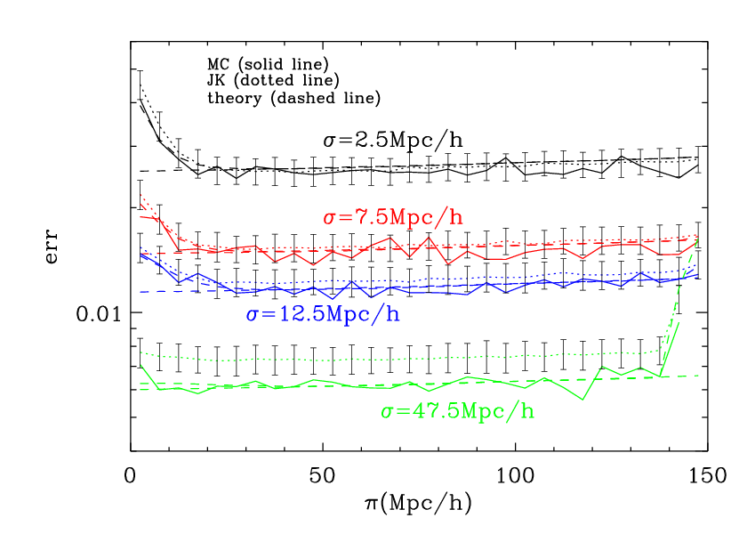
We study here the errors in the anisotropic redshift-space correlation function . The JK and MC errors only seem to agree at small perpendicular scales , which means that we can not use the JK error for large values. This is illustrated in Fig.21. The reason for this behaviour could partially be related to the fact that we have defined the JK zones in angular space, ie in the direction. As we increase the different JK zones are less independent. This could explain why JK errors do not work so well. In the radial direction, the different JK zones are more independent from each other and the JK errors give a better agreement to MC errors.
A.2.1 Error model
We have found a phenomenological model (we sometimes call it ”theory” or ”analytical” error) for the errors that match well the MC errors at large , even at large scales. The advantage of using a model is that is smoother than MC errors and can also be used to calibrate JK errors. We will first test this model in different situations.
Our ”theory error” has a dominant shot-noise contribution, which scales as , and a part proportional to the signal. This works well in this case because our LRG sample is shot-noise dominated, specially at large scales, and we are able to separate both contributions, as if we were in a diagonal space. In general, the analytical derivation of the error is more complicated that this simple modeling. We propose the error to have the following form , with two arbitrary coefficients and , so that:
| (31) |
adding these two terms linearly fits the simulations better than in quadrature. For Poisson shot-noise we have by definition that . This works very well for dark matter mocks, but we will show that groups do not follow the Poisson distribution and . We can associate to the number of independent nodes in the catalog and we therefore expect to scale with the square root of the volume of the sample used. We also expect to depend on the binning used. We use the estimator of Landy and Szalay (1993) to calculate the correlation function,
| (32) |
In the case of dark matter mocks, the error that comes from having a limited number of data-data (DD) pairs (Poisson shot-noise) is: , and for DR pairs: , where the random catalog is times denser than the data catalog. The error in random-random is insignificant, because we are using a denser random catalog. We add the different errors in quadrature to find:
| (33) |


We can reduce the error in by increasing the number of particles in the random catalog, modifying the error coming from DR, which is inversely proportional to the square root of the pairs data-random. The first part of the error is always the same, because it depends only on the data. For , as in the simulations, , so the DR part is 40% of the DD part. For , as in the analysis of LRGs, , so the DR part is now 20% of the DD part. For a binning of 5Mpc/h, we find and for binning of 1Mpc/h, . For Mpc/h, the signal part in is not very significant. This can be seen in Fig.21, where the linear dashed line correspond to the shot-noise term and the curved dashed line (only important on scales Mpc/h) also includes the signal part in Eq.(31). For small scales, JK and MC coincide, so we could just use JK error from the actual LRG data. In practice we prefer to use our model error to the JK error because this avoids introducing noise in the error analysis, but we have checked that none of our results depends on this choice.
A.2.2 Super-Poisson errors
In the case of groups, the Poisson model for the shot-noise does not work well. The reason for this is that groups are selected using friend-of-friends with linking length of times the interparticle separation. This means that groups create excluding regions where we can not randomly locate another group and therefore do not follow a Poisson distribution [Smith et al ¡2007¿]. Shot-noise is larger in this case, which we call ”super-Poisson”. After exclusion, the fraction of available volume is so we expect the Poisson term to be corrected by the square root of this fraction, ie roughly . This is exactly what we find for our model in Eq.(31) for group mocks. We have studied super-Poisson errors in two group simulations (z=0 and z=0.5) with the same linking length , and obtain the same value of , as expected, despite the large difference in the number density of groups.
What about real LRG galaxies? Do they follow the Poisson shot-noise or the groups shot-noise model? Real LRG data seems to follow more closely the group shot-noise as we find that we need rather than for Poisson term when we fit the JK errors in the real data at small . As we have seen with mocks, the JK errors reproduce very well the true errors for small both the Poisson (dark matter) and super-Poisson (groups). The amplitude of the JK errors on small is quite closer to group mocks than to dark matter mocks (this can be seen by comparing Fig.22 to Fig.23 below). This by itself is a very interesting result because it clearly shows that LRG galaxies have a tendency for exclusion. This suggests that a dominant fraction of LRG populate separate dark matter halos (this has already been studied with the same conclusions using semi-analytical models, Almeida et al 2008, or with real LRGs, Wake et al 2008 and Zheng et al 2008). It also shows that using dark matter mocks or a standard (Poisson) point process to simulate LRG will result in an important underestimation of errors.

A.2.3 Errors in LRG
Fig.22 shows the full 2D version of Fig.21. We show here the differences in the diagonal error between MC, JK and the theory error in Eq.(31), when binning the correlation function with 5Mpc/h. MC error is calculated using MICE simulation and JK is the mean over all the JK that we have calculated in each mock. JK errors work well for small Mpc/h but that become higher than MC when going to large for the reasons explained above. Our ”theory” error model form agrees with MC error at all scales, except in the radial direction, Mpc/h, for the case of group mocks (where we used a fixed at all ), which is slightly higher than the MC or the JK errors. The model for dark matter mocks, with does well at all . This can be seen in Fig.21. Thus in the radial direction we need to change for groups to , a lower value than . The reason for this is most probably the random component of peculiar velocities in redshift space, which ramdomizes the radial positions of group and reduces the super-Poisson shot-noise contribution, which comes from self-exclusion in group positions. This is no problem when analyzing real data as we can fit to match the JK error at small values of (with a different value at than at Mpc/h) and then use our error model for large values of where JK does not work well. We could also directly use the MC errors in the group mocks, which seem to agree quite well with real LRG data (ie JK errors are very similar in both cases, see Fig.23).
In Fig.23 we show the JK error obtained from the real LRG data using a random catalog 10 times denser than the data (as done with the mocks), and the analytical form with a fixed and . As in the mocks, for large the JK error is bigger than the analytical error, which should be more representative of the true (MC) error. At small scales the model follows the JK prediction, except for Mpc/h where we need to change to (the figure shows the model for at all ). Note the similarity between the errors in the data and in the group mocks in Fig.22. For our final analysis of the data we use a random catalog 20 times denser to reduce the error contribution due to the shot-noise in the randoms.
We have done a similar analysis with the L-BASICC halo simulations from Durham [Angulo et al ¡2008¿], which have approximately the same bias as real LRG in SDSS, and we find very good agreement with our fitting formula. If we use a random catalog 20 times denser, as we do for the analysis of the data, the error is lower, just as expected.
A.2.4 Covariance
So far we have shown diagonal errors. The normalized covariance is in fact quite small for dark matter mocks. It has the same approximate shape and amplitude for all the points. The amplitude of the covariance is just given by the distance between bins: at a separation of 5Mpc/h the normalized covariance is . This is also true for group mocks in the radial direction. But the covariance is larger in the case of groups for . At a radial distance of 5Mpc/h between bins in the normalized covariance is about 0.5 and dies below for bins separated by more than 15 Mpc/h. This is illustrated in Fig.24, which just shows the covariance in one of the bins. Other cases are very similar. The inner contour, which corresponds to for groups, is very similar in shape for dark matter and radial bins, but the amplitude in this case is 0.1.


If we bin the plane with 1Mpc/h, the same theory error form in Eq.(31) still works on all scales. So does the JK, at low . But in general errors are higher than when using a wider bin (smaller bin means smaller number of pairs). This increase is compensated by a decrease in the covariance, which becomes practically zero for all elements outside the diagonal.
A.3 Errors in the monopole
The error in the monopole is not easy to predict theoretically, but in this case JK error works very well for both variance and covariance on all scales. In the left panel of Fig.25 we plot the monopole when we bin the data with a separation 5Mpc/h: black for the dark matter mocks and red for LRG data (which will be presented in more detail in section 4). In the right panel, we see the difference between the mean JK error and its dispersion (solid line with errors) and the MC error (dashed line), and over-plotted the JK error for the real LRG (color). As can be seen, the error for LRG is larger than the one in simulations, since the signal is also higher, due to an overall bias in the amplitude. The small difference between blue and red line in Fig.25 is due to the number of the particles in the random catalog (), which does not change the estimation of the error in this case. Results are very similar for group mocks, with higher amplitudes, as expected. The important point here is that the JK error works well at all scales.


The normalized covariance, in Eq.(30), for the monopole is plotted in Fig.26. The result is not completely smooth for the MC case (top panel), because we need more than 216 simulations to have a smooth result. But we see that it has the same shape than JK covariance, which we will use to fit our LRG data. JK covariance is smoother than the MC because we have taken the mean over 216 x 63 realizations (216 mocks x 63 JK zones), which seems enough to converge. The bottom panel shows JK errors in the real LRG data, which is quite similar to the mocks, but looks noisier because this is just a single realization.
We have also binned the monopole with 1Mpc/h. JK error also works in this case, and we also see that the error is higher here than in the 5Mpc/h bin, while the covariance is smaller, practically equal to zero.
A.4 Error in the quadrupole Q(s)
For the quadrupole, the JK error also works quite well, as we can see in Fig.27 for 5Mpc/h (top panels) and 1Mpc/h binning (bottom panels). Again here , the solid line with errors shows the JK error and its dispersion, the dotted line is the MC error, and the color and lower line is the JK error in LRG data. The error for LRG data, in the quadrupole, is lower than the simulations one. This is because the error here is proportional to the signal, and in this case, LRG signal is lower since Q(s) depends on which depends inversely on bias . Results for group mocks are in good agreement with data and yield similar results for the comparison on JK and MC errors.
A.5 Validity of the models
We also use the simulations to test the methods that we will apply to real data (LRG) in the following sections. We want to study if we can recover the parameters that were input in the simulations.


A.5.1 Recovering the real-space correlation function
We first estimate the 2-point real-space and redshift-space correlation functions and compare to the input model that describes the simulation (see top panel in Fig.28). We find very good agreement. We look at the ratio between the redshift space and real space, which should be a function of the distortion parameter at large scales (and for the distant observer approximation), as in Eq.(23). In bottom panel of Fig.28 we have plotted the mean ratio over the simulated mocks, with its error, and over-plotted in red the expected value for the ratio at as in the input model. We also plot the mean()/mean() in dashed line (a biased estimator), which is similar to the mean() until 30Mpc/h. It seems to converge below 10Mpc/h and starts to fail around 30Mpc/h, where errors rapidily increase, which is in agreement with other analysis (see Fig.13 in Hawkins et al 2003). We could obtain from the ratio , but it is difficult in real data since we do not have direct information of the real-space , only through integration of the anisotropic through the line-of-sight (see §2.3). The advantage of using this ratio is that it converges to a constant value at small scales. But we can only use this below 30 Mpc/h with real data because the recovered real-space correlation function starts to fail on larger scales (see Fig.1). We have fitted these scales with the simulations and the results for are the ones expected. However, we have checked that it is better to obtain from the quadrupole Q(s), since it is more independent of other cosmological parameters and can be trusted to larger scales.
A.5.2 Fitting of the quadrupole Q(s) to obtain and
We can calculate the multipoles of to decompose the anisotropy between the LOS and the perpendicular direction. We have tested with models that the monopole and quadrupole and even the combination depend strongly not only on and , but also on other parameters like the shape of the correlation function (ie , and ), the non-linear bias and the overall amplitude. On the contrary, the reduced quadrupole Q(s), defined in Eq.(17) only depends strongly on and , but not on the bias. So when using the quadrupole we do not need an expression for the non-linear bias or a prior on (the shape of ) to extract the information. We can fix these parameters, and only change and . The asymptotic value of Q(s) for large scales in Eq.(18) is a function of , but it is always biased to higher values because of the random velocities. So it is dangerous to obtain from this asymptotic approximation. We instead generate our model for Q(s) based on the multipoles of in Eq.(16) and Eq.(17).




For the dark matter mocks we have that (see §A) and is approximately 400km/s on large scales, but higher when approaching scales smaller than 10 Mpc/h (see Fig.29). We fit the quadrupole obtained for each mock separately. The mean over all the mocks gives the correct exact value of and a value of 450Km/s which is slightly larger than the asymptotic large scale value of 400 Km/s. This is probably because we are obtaining an effective which also accounts for the values at lower scales which are larger, as shown in Fig.29. But at (2 dof) 450Km/s is consistent with the asymptotic value at large scales, which is plotted as a red dot in Fig.30. In Paper-II of this series we show how to find the exact value for as a function of scale.
In the top panel in Fig.30, we show the mean contour which is the average over the individual contours in each simulation, obtained from . In the bottom panel, we show the best fit model over-plotted over the mean Q(s) with the MC errors. The MC errors here correspond to a single mock, while errors in the mean value are times smaller (N=216 in our simulations). In the bottom panel of Fig.30, we plot the errors corresponding to a single mock. We find similar results for group mocks, which have different values of . We conclude that the model used for the quadrupole, assuming a constant , is perfect to obtain and an effective which does not have to correspond necessarily to the large scale value, but rather to a combination of at different scales.
A.5.3 Fitting of large scales: and amplitude
From large scales, we will obtain the shape of the linear correlation function . Here we will only fit and the amplitude of the correlation. We have fixed , and following recent results of WMAP, SNIa and previous LSS analysis 44 4 see http://lambda.gsfc.nasa.gov/product/map/dr3/parameters.cfm.
As we have seen in §2.3 we can not rely on the projected correlation function at large scales, or the recovered real space correlation function, so the way to extract information about the shape of the real space correlation function is directly from . We use models that vary with , linear amplitude, and . The linear amplitude refers to the factor , where b(z) is the bias at redshift z. and are completely degenerated in the correlation function, also with the growth factor . In fact, what we obtain from observations is , but D(z) is known for each cosmology and the median redshift of the slice. We have checked with simulations that we can use linear bias in the scales that we are interested. We also use the priors and found previously from the normalized quadrupole, although this does not make a large difference. Then, we need to fit and . The best place to fit them, so that is independent on scale, is for intermediate scales, from 20Mpc/h to 60Mpc/h, to be safe from non-linear bias. We also stay away from the line-of-sight (LOS) where fingers of God can alter the information, cutting an angle of 30-40 deg away from the LOS when doing the fit. We marginalize over and obtain a contour for which is in very concordance with the input values. Although obtained from Q(s) is just an effective value, simulations show that we recover the correct value of . We can understand it, because does not play an important role in our selected range of scales in . If we extend to larger distances, the value for is biased slightly to lower values, probably because of the wide angle effect. This is important for an angle of 10 deg between galaxies [Matsubara ¡2000¿], which is more than 70Mpc/h for our worst case (z=0.15), in the perpendicular direction .
A.5.4 Model for the 2-point correlation function
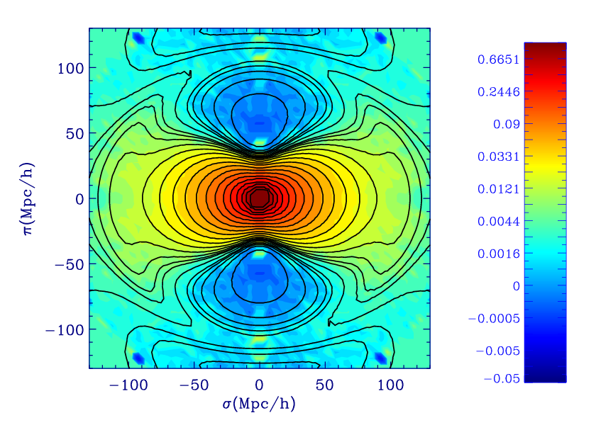
Finally, in Fig.31, we plot at large scales for the mean over MICE mocks (colors). We over-plot in solid lines the best model (using Eq.(14)). In all cases, we use an effective . Note that we use square bins (pixels) of 5Mpc/h side at all scales and this dilutes the FOG at small . The model works very well compared to simulations. We can observe in the figures that the overall amplitude is different for each simulation, because it is proportional to the bias. The same bias modifies the distortion parameter (inverselly proportional to the bias) which changes the shape of . The larger the value of the greater squashing effect in the radial () direction. Also note the closed contours in the radial direction between Mpc/h (in dark blue). They correspond to a region of negative amplitude caused by the squashing (Kaiser) effect. The larger the value of the larger the region with negative values. This region is sorounded by the BAO ring at about 100 Mpc/h. It is remarkable how well this is followed by simulations, which indicates that this is a very significant feature. We have shown before that data also follows this feature.
Simulations also show a good agreement with the BAO peak, including some detection in the radial direction which is enhanced by noise. This will be studied in more detail in Paper IV of this series.
We see that the obtained correlation (colored) differs slightly from the distant observer approximation theory (lines) at large and . The redshift space correlation distortion in real surveys, which are not located at infinity, depends on and , but also on the angle between galaxies and the angle between the direction LOS (at ) and the vector which goes from galaxy 1 to galaxy 2 (following the notation used in Matsubara 2000). In the distant observer approximation we assign to the angle between galaxies the value . Matsubara (2000) has studied the differences between the real correlation and the approximation for distant observers. In general, the approximation is good for angles below 10 deg, which include all the zone we are using for our analysis in LRG data (the worst case comes from the closest galaxies at z=0.15, where corresponds to ). The correlation also depends on the angle. We can see in Fig.9 of Matsubara (2000) a comparison between the real correlation, which depends on the distance between galaxies and both angles described above, and the distant observer correlation function, used in this work, which depends only on and . Each position in the 2 dimensional is a mixing of different and , because there is a range in redshift, but we can explain qualitatively the lack of power of the observed correlation respect to the distant observer approximation theory at large and .
We have also calculated the correlation function limiting the angle between galaxies to see in practice how is affected by wide angle effects (see Appendix B5). As we increase the restriction, we see how the direction recovers power in better agreement with the model predictions. In real data, we rather use all pairs given that this is quite a small distortion.
Appendix B Systematic effects
In this section we look for possible systematic errors that could be imprinted by the radial mask through the line-of-sight, the angular mask, or the selection of LRGs . These systematic effects are typically more important on the largest scales, where the correlation function becomes smaller. In Fig.19 we show that for some slices there is extra power in at scales , something which is not expected in the models. This is particularly evident for the slice in redshift z=0.3-0.4, where the signal-to-noise is small ( and bias are smaller in Table 2) and we do not have a significant peak detection. This extra power could be due to sampling variance but could also be caused by some systematic errors in the data or the way we analyze it. The extra power seems to be important at scales larger than the baryonic peak, but we test here if it could also have some effect over the peak location. This extra power have also been detected in other analysis of SDSS LRG around similar scales [Blake et al ¡2007¿, Padmanabhan et al ¡2007¿]. We will focus here on systematics related to the way we have analyzed the data, rather than systematics in the data itself. The later has been explored in detail elsewhere [Eisenstein et al ¡2005¿].
B.1 Radial Selection
First, we test the radial selection function that we use for the random catalogs. If we use exactly the same radial density distribution as selection function of the data, we suppress the radial modes in the direction. In Fig.32 we can see the differences between different smoothing windows in the data selection function, and in Fig.33 and Fig.34 the redshift-space correlation function for these three smoothing bins.


We do not see any significant difference between the three cases indicating that our analysis is robust with respect to the radial selection.
B.2 Weighting
In Fig.35 we compare our results
in the monopole (red with shaded region as errors) to that of
Eisenstein et al (2005) (in black line with errorbars) for all the sample.
Our result is consistent with this previous estimate despite the increase
in the DR6 area and the
difference in the selection. However, at larger scales than the baryonic
peak, we observe some extra-power in our estimation.
We wonder if the difference is just due to sampling, selection
or to the way we estimate the correlation function (we do not include
the same weighting as Eisenstein et al 2005)

We have also calculated the correlation function using a weighting scheme, as the one explained in Eisenstein et al (2005). We weight the sample using a scale-independent weighting that depends on redshift. When computing the correlation function, each galaxy and random point is weighted by 1/(1 + n(z)Pw) [Feldman et al ¡1994¿] where n(z) is the comoving number density and . We do not allow Pw to change with scale so as to avoid scale-dependent changes in the effective bias caused by differential changes in the sample redshift. We choose Pw at as in Eisenstein et al (2005). At z 0.36, nPw is about 4, while at z = 0.47.

In Fig.36 we can see the comparison between the correlation function estimated without weighting (solid line) and with weighting (dashed line). Contrary of what we were looking for, the extra power is higher in the weighting scheme, which makes sense, since we are now giving more importance to the higher redshift pairs, which have a larger bias (see below).


In Fig.37 we have plotted the anisotropic correlation function for both cases, showing only slight differences. It is apparent that the monopole is more sensitive that to displace systematic differences. We will therefore concentrate on results for the monopole from now on.
B.3 Angular Selection
We next look at the angular selection function, the mask. First, we construct a different mask than the original by using a Healpix map [Górski et al ¡2005¿], with nside=64 (with pixels of area 0.8 sq deg). In Fig.38 we plot the distribution function for the number of galaxies per pixel. The pixel is large enough to distinguish between real empty pixels and artificial ones. We only include pixels that have more than n galaxies, where n=2,6 and 10. As we can see in the distribution plot, if we include more than 2 galaxies, we are probably including artificially void zones, which will create extra power and pencil beams at the direction line-of-sight, while when we include only the pixels with more than 10 galaxies, we are probably excluding some real voids. In this second case, the density is higher than the real one, so the density contrast is lower. We can see these effects in Fig.39 for the correlation function in redshift space. We see that the correlation is lower when we increase the minimum number of galaxies (from red to blue), but we can always see the baryonic peak and the three lines have the same shape approximately. Our results are similar to the case n 6, which does not include artificial voids and does not eliminate real voids.


The spectroscopic survey of SDSS is observed using circular plates,
which contain about 600 fibers each to take spectra. Targets are selected
from the photometric survey, although the spectroscopic survey is not exactly
the same as the photometric one. There are some plates that have not been
observed properly due to known problems, which are explained in the
web (http://www.sdss.org). We have extracted from our previously
calculated mask all the galaxies that are not laying inside “good”
plates (maskplate1). In Fig.40 we can see the plates
(black circles) and the galaxies (red dots). Moreover, we can also eliminate
all the galaxies that lay inside a bad plate to ensure that we are taking
only the really good ones (maskplate2). This second mask reduces the number
of galaxies significantly, and the correlation is then a lot noisier, but
we show here the results. In Fig.41 we have plotted
the redshift-space averaged correlation function for the new mask based
on spectroscopic plates. Results are very similar to our previous result,
in black. Moreover, we over-plot the result for the north stripe of SDSS,
which contains the most significant part of the survey, in blue. The anisotropic
redshift-space correlation function is really similar in all these cases,
so that we do not find it useful to plot it.


We have also tried to extract all the plates that have a large number of galaxies,
which have big superclusters, since it is known that big clusters can bias
the correlation function for regular galaxies [Baugh et al ¡2004¿]. The result is not significantly modified
which could have been expected since LRG in SDSS DR6 cover a much larger volume
that 2DFGRS or SDSS for regular galaxies.
B.4 Volume limited samples
In volume limited surveys, we can estimate the correlation function with a pixelization scheme. The correlation function can then be estimated as:
| (34) |
where and the sum extends to all pairs i,j
separated by a distance . We have taken a volume limited
part of the selected galaxies, with redshift z=[0.15,0.38] and absolute
magnitude =[-22.5,-21.5] and have calculated the correlation using
this method. This is the same sample used in Paper IV of this series.
We have also calculated a similar selection by using the
traditional method with a random catalog. Results are plotted in
Fig.42, dotted for the pixel method and solid
for the randoms. This is a good test to validate our results, since both methods
are quite different. As we can see in the figure, the
two estimations are very similar. The slight shift in amplitude at
small scales is due to the pixel
smoothing, a cube of 10 Mpc/h on the side for this case. This shift can
be modeled with a top-hat window function reproducing the exact
amplitude difference. There is a very good match
using smaller pixel size. Also note how these estimations, based on a volume limited
sample with about half of the LRG galaxies, agree quite well
with previous results (ie in Fig.41) which
includes all galaxies at a price of a more complicated selection function.
Despite all this difference, we see no significant
change in at the largest scales.

We have also divided the catalog in different volume limited slices as indicated in table 3 plotted in Fig.43. The most and least luminous slices (in the bottom right and top left) contain fewer galaxies and have too much noise at the baryonic peak, but we see that the red and pink slices, at intermediate redshifts and magnitudes, contribute to the extra-power that we see at large scales (Fig.44 with the same colors as Fig.43). Note how these subsamples cover a sharp feature a z=0.35 in the selection function (eg see Fig.32) which is clearly an artifact of the selection function because of the double selection cut in LRG. This feature is diluted when we consider volume limited samples as we discard the less luminous galaxies which contribute most to this peak. As shown above, the correlation for a volume limited sample in the range =[-22.5,-21.5], shown in Fig.42 is in excellent agreement with the one for the whole sample in Fig.35. Thus we conclude that our measurements are quite robust and are not affected by the selection cuts.
| Sample | M-range | Mean M | mean z | z-range |
|---|---|---|---|---|
| S22.50 | -22.50 -23.00 | -22.75 | 0.43 | 0.35-0.50 |
| S22.25 | -22.25 -22.75 | -22.50 | 0.40 | 0.33-0.48 |
| S22.00 | -22.00 -22.50 | -22.25 | 0.38 | 0.31-0.46 |
| S21.75h | -21.75 -22.25 | -22.00 | 0.35 | 0.27-0.42 |
| S21.75 | -21.75 -22.25 | -22.00 | 0.20 | 0.12-0.27 |
| S21.50h | -21.50 -22.00 | -21.75 | 0.32 | 0.25-0.40 |
| S21.50 | -21.50 -22.00 | -21.75 | 0.18 | 0.10-0.25 |
| S21.25 | -21.25 -21.75 | -21.50 | 0.18 | 0.10-0.25 |


We have not plotted larger scales for the
other slices because they are quite noisy. However, at intermediate scales, we can see clearly
the bias due to different intrinsic luminosity, more biased when more luminous, although bias
seems to be independent on scale, in the scales used for our analysis.
B.5 Wide angle approximation
We have calculated the correlation function limiting the angle between galaxies to see
if wide angle effects that are apparent in disappear. In Fig.45, we see the anisotropic
without limits in the angle (top panel) compare to the one
only accepting galaxies with
(bottom panel). As we increase the restriction, we see
how the direction recovers power, which explains the lack of power we saw in the
direction when angles are too big to apply the distant observer approximation.
The angle between galaxies explain part of the distortions due to wide angle effects,
specially the ones that are concentrated at small and large , which affect
the first slice considered, from z=0.15-0.3. The angle , between the direction
LOS (at ) and the vector which goes from galaxy 1 to galaxy 2 (following the
notation used in
Matsubara 2000), is also important and can also imprint some
modifications at larger and large .


We conclude that the measurements on the BAO scale are quite robust and the extra power at the largest scales is probably the result of sampling fluctuations and shot noise. For redshifts around z=0.35 we find extra noise on large scales, probably due to an artifact in the selection function. In any case, none of the systematics we have explored modify the peak detection in a significant way.