Spin, charge and single-particle spectral functions of the one-dimensional quarter filled Holstein model.

F. F. Assaad Affiliation: Institut für theoretische Physik und Astrophysik, Universität Würzburg, Am Hubland, D-97074 Würzburg, Germany

Abstract

We use a recently developed extension of the weak coupling diagrammatic determinantal quantum Monte Carlo method to investigate the spin, charge and single particle spectral functions of the one-dimensional quarter-filled Holstein model with phonon frequency $\omega_{0}=0.1t$ . As a function of the dimensionless electron-phonon coupling we observe a transition from a Luttinger to a Luther-Emery liquid with dominant $2k_{f}$ charge fluctuations. Emphasis is placed on the temperature dependence of the single particle spectral function. At high temperatures and in both phases it is well accounted for within a self-consistent Born approximation. In the low temperature Luttinger liquid phase we observe features which compare favorably with a bosonization approach retaining only forward scattering. In the Luther-Emery phase, the spectral function at low temperatures shows a quasiparticle gap which matches half the spin gap whereas at temperatures above which this quasiparticle gap closes, characteristic features of the Luttinger liquid model are apparent. Our results are based on lattice simulations on chains up to L=20 for two-particle properties and on CDMFT calculations with clusters up to 12 sites for the single-particle spectral function.

pacs

71.27.+a, 71.10.-w, 71.10.Fd

I Introduction

Including phonon degrees of freedom in model calculations of correlated electron systems is challenging but necessary for the understanding of many experiments. One can mention the quasi one-dimensional organics TTF-TCNQ where photoemission experiments are carried out down to 60 K just above the Peierls transition [1]. A detailed modeling of this experimental situation is bound to include both electronic correlations [2, 3, 4, 5] as well as the phonon degrees of freedom [6]. In two dimensions the electron-phonon interactions leads to a delicate interplay of superconductivity and charge density waves depending on the partial nesting properties of the Fermi surface [7, 8]. More generally, the ability to efficiently include bosonic baths in Quantum Monte Carlo (QMC) simulations is a prerequisite for the implementation of extended dynamical mean-field theories (EDMFT) where self-consistency both at the two particle (bosonic baths) and single particle levels is required [9, 10].

The aim of this article is to test on the basis of a non-trivial model a recently proposed generalization of the weak coupling diagrammatic determinantal QMC algorithm to include phonon degrees of freedom [11, 12]. The approach relies on integrating out the phonon degrees of freedom at the expense of a retarded interaction and then to expand around the non-interacting point. Classes of diagrams at a given expansion order can be expressed in terms of a determinant, the entries of the matrix being the non-interaction Green function. The summation over those classes of diagrams is carried out with stochastic methods. Since the algorithm action based, the CPU time scales as $(\beta L)^{3}$ ( $\beta$ is the inverse temperature and $L$ the number of lattice sites ) and is easily embeded in dynamical mean-field self-consistency loops. To obtain a full account of the physics, we have carried out lattice simulations on lattices up to $L=20$ to extract two particle quantities and cluster dynamical mean-field theory (CDMFT) [13] calculations on embedded clusters up to $L_{c}=12$ to investigate the single particle spectral function. As a function of the dimensionless electron-phonon coupling and at fixed phonon frequency $\omega_{0}/t=0.1$ , we interpret our low temperature results in terms of a transition from a Luttinger liquid with gapless spin and charge modes to a Luther-Emery liquid with gapful spin and gapless charge modes [14]. This Peierls phase has dominant $2k_{f}$ charge density wave (CDW) correlations. We have placed emphasis on the temperature dependence of the single-particle spectral function in both phases. At high temperatures and in both phases the QMC data compares favorably with a self-consistent Born approximation [15]. The low temperature properties in the Luttinger liquid phase compare favorably to a bosonization approach retaining only forward scattering [16] whereas in the Luther-Emery phase a quasiparticle gap matching half the spin gap is apparent. The temperature dependence of the single particle spectral function in the Luther-Emery phase is particularly rich; at temperature scales where the quasiparticle gap closes, features of the Luttinger liquid model are apparent.

The article is organized as follows. In the next section we introduce the model, and briefly review our implementation of the CDMFT. We refer the reader to Ref. [12] for a detailed description of the QMC method. In Section III we present our numerical results for two-particle and single particle correlation functions across the Peierls transition. For completeness sake, two appendices summarize the self-consistent Born approximation [15] and elementary aspects of the the Luttinger model appropriate for the description of the low-energy excitations of the Luttinger liquid phase [16].

II Model and Quantum Monte Carlo.

The one-dimensional Holstein model we consider reads:

\hat{H}=\sum_{\boldsymbol{k},\sigma}\epsilon({\boldsymbol{k}})\hat{c}^{\dagger}_{{\boldsymbol{k}},\sigma}\hat{c}_{{\boldsymbol{k}},\sigma}+g\sum_{\boldsymbol{i}}\hat{Q}_{\boldsymbol{i}}\hat{n}_{{\boldsymbol{i}}}+\sum_{\boldsymbol{i}}\frac{\hat{P}_{\boldsymbol{i}}^{2}}{2M}+\frac{k}{2}\hat{Q}_{\boldsymbol{i}}^{2},

(1)

with tight binding dispersion relation $\epsilon({\boldsymbol{k}})=-2t\cos({\boldsymbol{k}}{\boldsymbol{a}})-\mu$ . $\hat{c}^{\dagger}_{{\boldsymbol{i}},\sigma}$ creates an electron in Wannier state centered on lattice site ${\boldsymbol{i}}$ and with z-component of spin $\sigma$ , $\hat{c}^{\dagger}_{{\boldsymbol{k}},\sigma}=\frac{1}{\sqrt{L}}\sum_{{\boldsymbol{i}}}e^{i{\boldsymbol{k}}\cdot{\boldsymbol{i}}}\hat{c}^{\dagger}_{{\boldsymbol{i}},\sigma}$ creates an electron in a Bloch state with crystal momentum ${\boldsymbol{k}}$ , $\hat{n}_{{\boldsymbol{i}}}=\sum_{\sigma}\hat{c}^{\dagger}_{{\boldsymbol{i}},\sigma}\hat{c}_{{\boldsymbol{i}},\sigma}$ is the on-site particle number operator and $\hat{Q}_{\boldsymbol{i}}$ and ${\hat{P}}_{\boldsymbol{i}}$ corresponds to the ion displacement and momentum.

In a recent publication [12], we have shown how include phonon degrees of freedom in the weak coupling diagrammatic determinantal quantum Monte Carlo (DDQMC) algorithm [11]. The key ingredient is to integrate out the phonon degrees of freedom at the expense of a retarded interaction and then to expand around the non-interacting limit. We refer the reader to Ref. [12] for a detailed description of the algorithm.

Since dynamical two particle quantities are notoriously hard to compute within cluster methods [17], we have used the DDQMC method to simulate the Holstein model on lattices up to $L=20$ sites to compute those quantities. For the study of the temperature dependence of the single particle spectral function, we have found it more convenient to adopt the cluster dynamical mean field theory (CDMFT) on embeded cluster sizes up to $L_{c}=12$ .

CDMFT as opposed to the dynamical cluster approximation (DCA) is particularly useful to tackle our problem. It is a real space method which allows for spontaneous symmetry breaking within a predefined unit cell of volume given by the cluster size. To implement the method, we decompose the chain into $L_{u}$ , super-cells of length $L_{c}$ . A site, ${\boldsymbol{i}}$ in the original lattice then corresponds to a super-cell, ${\boldsymbol{R}}$ , and an orbital index $\nu$ running from $1\cdots L_{c}$ such that: ${\boldsymbol{i}}={\boldsymbol{R}}+{\boldsymbol{a}}_{\nu}$ . Thereby, the volume of the Brillouin zone is reduced by a factor $L_{c}$ and the quantized wave vectors are given by ${\boldsymbol{K}}=\frac{2\pi}{L_{c}L_{u}}n$ with $n\in[-L_{u}/2,L_{u}/2[$ . Within this formulation, the self-energy and non-interacting Green function correspond to $L_{c}\times L_{c}$ matrices, ${\boldsymbol{\Sigma}}({\boldsymbol{K}},i\omega_{m}),{\boldsymbol{G}}_{0}({\boldsymbol{K}},i\omega_{m})$ . The CDMFT approximation neglects the ${\boldsymbol{K}}$ dependency of the self-energy; ${\boldsymbol{\Sigma}}({\boldsymbol{K}},i\omega_{m})\equiv{\boldsymbol{\Sigma}}(i\omega_{m})$ . In analogy to the DMFT approach, one can extract the self-energy by solving on an $L_{c}$ cluster the model at hand subject to a dynamical bath ${\boldsymbol{\cal G}}_{0}(i\omega_{m})$ which has to be determined self-consistently. To be more precise:

	$\displaystyle{\boldsymbol{\cal G}}(i\omega_{m})$	$\displaystyle=$	$\displaystyle\frac{1}{{\boldsymbol{\cal G}}^{-1}_{0}(i\omega_{m})-{\boldsymbol{\Sigma}(i\omega_{m})}}$		(2)
		$\displaystyle=$	$\displaystyle\frac{1}{L_{u}}\sum_{K}\frac{1}{{\boldsymbol{G}}_{0}^{-1}(K,i\omega_{m})-{\boldsymbol{\Sigma}}(i\omega_{m})}.$		(2)

The last equality corresponds to self-consistency. Hence, for a given bath Green function matrix ${\boldsymbol{\cal G}}_{0}(i\omega_{m})$ we use the DDQMC method to obtain the corresponding self-energy ${\boldsymbol{\Sigma}}(i\omega_{m})$ which in turn, owing to Eq. (2), allows us to compute a new bath Green function. This procedure is repeated till convergence is reached. Within the DDQMC the self-consistency is particularly easy to implement as it is possible to compute the Matsubara Green functions directly within the QMC code thus avoiding the cumbersome transformation from imaginary time to Matsubara frequencies.

Having determined the self-energy, we compute the lattice Green functions, $g({\boldsymbol{k}},i\omega_{m})$ and ${\boldsymbol{k}}\in\left[-\pi,\pi\right]$ with:

\begin{gathered}g({\boldsymbol{k}},i\omega_{m})=\\ \frac{1}{L_{c}}\sum_{\mu,\nu=1}^{L_{c}}e^{i{\boldsymbol{k}}\left({\boldsymbol{a}}_{\mu}-{\boldsymbol{a}}_{\nu}\right)}\left[\frac{1}{{\boldsymbol{G}}_{0}^{-1}({\boldsymbol{K}},i\omega_{m})-{\boldsymbol{\Sigma}}(i\omega_{m})}\right]_{\mu,\nu}.\end{gathered}

(3)

In the above, ${\boldsymbol{k}}={\boldsymbol{K}}+m\frac{2\pi}{L_{c}}$ with ${\boldsymbol{K}}\in\left[-\frac{\pi}{L_{c}},\frac{\pi}{L_{c}}\right]$ . We use CDMFT solely to extract the single particle spectral function. The required rotation from the imaginary to real time axis is accomplished with a stochastic analytical continuation scheme [18, 19].

III Numerical Results

In this section, we present our numerical results at quarter filling, $\rho=0.5$ , phonon frequency $\omega_{0}=0.1t$ , which places us in the adiabatic limit, and vary the electron-phonon coupling as well as the temperature. We first consider spin, charge and pairing correlations as well as the optical conductivity and then study in detail the temperature dependence of the single particle spectral function. Two particle quantities are obtained from simulations on an $L=20$ site lattice. To at best study single particle properties, we have used the CDMFT approximation on cluster sizes up to $L_{c}=12$ .

To characterize the strength of the electron-phonon interaction, we consider the effective mass renormalization as obtained from the self-energy diagram shown in Fig. 9. For a flat band of width $W$ , Eq. (21) yields:

\frac{m^{*}}{m}=1+\lambda\;\;{\rm with}\;\;\lambda=\frac{g^{2}}{2k}\frac{2}{W}

(4)

with $\lambda$ the dimensionless electron-phonon coupling.

III.1 Spin and charge static and dynamical structure factors.

Refer to caption — Figure 1: Density (a), pairing (b), spin (c) correlation functions as well as the single particle occupation number (d) as a function of electron-phonon coupling.

Equal time charge correlation functions,

N({\boldsymbol{q}})=\sum_{\boldsymbol{r}}e^{i{\boldsymbol{q}}{\boldsymbol{r}}}\left(\langle\hat{n}_{\boldsymbol{r}}\hat{n}_{0}\rangle-\langle\hat{n}_{\boldsymbol{r}}\rangle\langle\hat{n}_{0}\rangle\right),

(5)

are plotted in Fig. 1a. As a function of growing electron-phonon coupling, the cusp at $2k_{F}=\pi/2$ , signaling a power-law decay of the correlation function [20], evolves towards a clear peak signaling a dominant $2k_{F}$ charge modulation at $\lambda=0.35$ . Note that at the largest considered electron-phonon coupling, a cusp at a higher harmonic, $4k_{F}$ , is equally apparent. A simple interpretation of this charge-density wave stems form the Peierls instability. For classical phonons the inherent $2k_{f}$ nesting instability of one-dimensional systems renders the metallic state unstable towards a $2k_{f}$ lattice deformation at arbitrarily small electron phonon coupling. In this mean-field approach the static lattice deformation triggers the opening of a charge gap. It has been argued and shown numerically [21] that this situation cannot be carried over to quantum phonons. In this case, quantum fluctuations destroy the static lattice deformation and a finite value of the electron-phonon coupling is required to destabilize the Luttinger liquid. The linear behavior of the charge structure factor at long wavelengths (see Fig. 1a) points to a metallic state at all considered values of the electron-phonon interaction since it amounts to a powerlaw decay with modulation ${\boldsymbol{q}}=0$ of the real space charge correlation function.

Since we have not included a Coulomb repulsion in our model Hamiltonian, one expects two electrons of opposite spins to share the same lattice deformation and thereby bind to form bipolarons. Fig. 1b plots the equal time pairing correlation functions in the on-site s-wave channel,

P({\boldsymbol{r}})=\langle\hat{\Delta}^{\dagger}_{{\boldsymbol{r}}}\hat{\Delta}_{{\boldsymbol{0}}}\rangle\;\;{\rm with}\;\;\hat{\Delta}^{\dagger}_{\boldsymbol{r}}=\hat{c}^{\dagger}_{{\boldsymbol{r}},\uparrow}\hat{c}^{\dagger}_{{\boldsymbol{r}},\downarrow}.

(6)

As apparent, the on-site pairing correlations, $P({\boldsymbol{r}}=0)$ , grow as the electron-phonon coupling is enhanced from $\lambda=0.25$ to $\lambda=0.35$ . This behavior reflects the formation of bipolarons. On the other hand and in this coupling range, the long range pairing correlations are suppressed reflecting a tendency towards localization of the bipolarons.

The binding of electrons into spin singlets leads to the suppression of the $2k_{F}$ spin-spin correlation functions defined by

S({\boldsymbol{q}})=\sum_{\boldsymbol{r}}e^{i{\boldsymbol{q}}{\boldsymbol{r}}}\langle\hat{S}_{z,\boldsymbol{r}}\hat{S}_{z,{\boldsymbol{0}}}\rangle

(7)

and plotted in Fig. 1c. At $\lambda=0.35$ both the $q=0$ as well as the $q=2k_{F}$ cusps in the spin structure factor are smeared out thus lending support to an exponential decay of the spin-spin correlation.

Finally, the single particle occupation number,

n({\boldsymbol{k}})=\sum_{\sigma}\langle\hat{c}^{\dagger}_{{\boldsymbol{k}},\sigma}\hat{c}_{{\boldsymbol{k}},\sigma}\rangle,

(8)

is plotted in Fig. 1d. As apparent, and on our limited lattice size, $L=20$ , the jump at $k_{F}=\pi/4$ is dramatically suppressed as the electron phonon-interaction grows from $\lambda=0.25$ to $\lambda=0.35$ .

Hence, on the basis of the static quantities, we can conclude that a transition between a Luttinger liquid metallic phase and a spin gaped CDW state occurs in the region $0.25<\lambda<0.35$ . We now provide further support for this picture by examining dynamical two-particle correlation functions.

In the Lehmann representation, the dynamical charge susceptibility is given by:

N({\boldsymbol{q}},\omega)=\frac{\pi}{Z}\sum_{n,m}e^{-\beta E_{m}}|\langle n|\hat{n}_{\boldsymbol{q}}|m\rangle|^{2}\delta(E_{n}-E_{m}-\omega)

(9)

where $\hat{n}_{\boldsymbol{q}}=\frac{1}{\sqrt{N}}\sum_{j}e^{i\boldsymbol{q}{\boldsymbol{j}}}\hat{n}_{\boldsymbol{j}}$ and the sum rule $N({\boldsymbol{q}})=\frac{1}{\pi}\int d\omega N({\boldsymbol{q}},\omega)$ holds. A similar definition holds for the dynamical spin structure factor $S({\boldsymbol{q}},\omega)$ .

In the absence of the electron-phonon coupling, both spin and charge dynamical structure factors are identical and correspond to the well know particle-hole continuum with gapless excitations at ${\boldsymbol{q}}=0$ and ${\boldsymbol{q}}=2k_{F}$ . Note that at quarter-band filling, $2k_{F}=\pi/2$ . As apparent from the Luttinger liquid model (see Appendix B), the phonon mode couples only to the charge degrees of freedom. At weak couplings, $\lambda=0.15$ , the dynamical charge structure factor in Fig. 2 shows precisely this feature; the continuum of charge excitations is supplemented by the dispersionless phonon mode at $\omega_{0}=0.1t$ . In the spin sector (see Fig. 3) only the continuum of two spinon excitations is present.

At larger values of $\lambda$ ( $\lambda=0.35$ ) and as a consequence of the bipolaron formation spectral weight at low energies in the dynamical spin structure factor is suppressed. In particular from Fig. 3 we can obtain a rough estimate of the spin gap at, $\Delta_{sp}\simeq 0.2t$ at $\lambda=0.35$ . The lattice distortion in the Peierls phase is accompanied by a softening of the phonon mode. At $\lambda=0.35$ (see Fig. 2) we observe a piling up of spectral weight at very low frequencies with dominant spectral intensity at ${\boldsymbol{q}}=2k_{F}$ . This low energy feature corresponds to the slow charge dynamics of the bipolaronic $2k_{f}$ CDW (see Fig. 1a) ¹¹ 1 This slow dynamics of the bipolarons is at the origin of long autocorrelation times observed in the QMC simulations at large values of $\lambda$ .. The high-energy continuum at $\lambda=0.35$ in $N({\boldsymbol{q}},\omega)$ is comparable to $S({\boldsymbol{q}},\omega)$ at the same coupling. This similarity confirms that this structure stems from the particle-hole bubble of dressed single particle Green functions.

We note that phonon dynamics have been studied for the spinless Holstein model within a projector based renormalization method [22] as well as with exact diagonalization and CPT methods [23]. In analogy to our results, the phonon spectral function reveals not only the phonon dynamics but also the particle-hole continuum.

Finally we consider the real part of the optical conductivity,

\sigma^{\prime}(\omega)=\frac{\pi}{Z\omega}\sum_{n,m}e^{-\beta E_{m}}(1-e^{-\beta\omega})|\langle n|\hat{j}|m\rangle|^{2}\delta(E_{n}-E_{m}-\omega)

(10)

with $\hat{j}=it\sum_{{\boldsymbol{i}},\sigma}\left(\hat{c}^{\dagger}_{{\boldsymbol{i}},\sigma}\hat{c}_{{\boldsymbol{i}}+{\boldsymbol{a}},\sigma}-{\rm H.c.}\right)$ both at $\lambda=0.15$ and $\lambda=0.35$ . Our results on an $L=20$ lattice are plotted in Fig. 4. As apparent at $\lambda=0.15$ a Drude feature reflecting polaronic conductivity is visible. In contrast, at larger electron-phonon couplings, the formation of the bipolaronic CDW leads to a substantial suppression of the Drude feature. The suppression of the Drude weight reflects the very small charge velocity of the bipolarons. This follows from the continuity equation which establishes a relation between the optical conductivity and the dynamical charge structure factor:

\sigma^{\prime}({\boldsymbol{q}},\omega)=\frac{\omega}{{\boldsymbol{q}}^{2}}\left(1-e^{-\beta\omega}\right)N({\boldsymbol{q}},\omega).

(11)

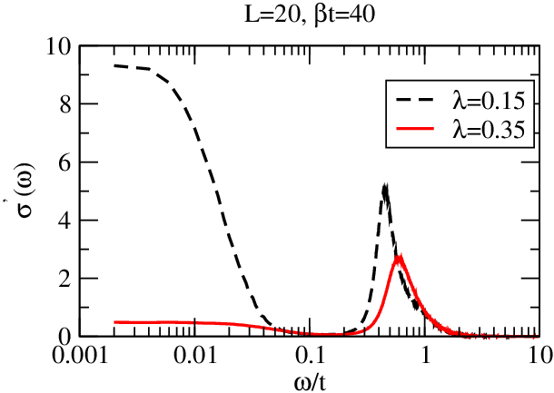
At small momentum transfer, and using the sum rule $\frac{1}{\pi}\int{\rm d}\omega N({\boldsymbol{q}},\omega)=N({\boldsymbol{q}})$ , we can model the dynamical charge structure factor by: $N({\boldsymbol{q}},\omega)=\pi N({\boldsymbol{q}})\delta(v_{c}{\boldsymbol{q}}-\omega)$ with $v_{c}$ the charge velocity. From Fig. 1a $N({\boldsymbol{q}})\propto{\boldsymbol{q}}$ in the long wavelength limit, and the proportionality constant is to a good approximation $\lambda$ independent. Inserting this approximate form of into Eq. (11) gives in the zero temperature limit:

\lim_{{\boldsymbol{q}}\rightarrow 0}\sigma^{\prime}({\boldsymbol{q}},\omega)\propto v_{c}\delta(\omega).

(12)

Hence, the suppression of the Drude weight stems from reduction of the charge velocity when passing from the Luttinger liquid phase to the bipolaronic CDW phase.

III.2 Temperature dependence of the single particle spectral function

In this section we study the details of the temperature dependence of the single particle spectral function, both in the Luttinger and bipolaronic CDW phases.

III.2.1 Atomic limit

It is instructive to start with the atomic limit, $t=0$ , and in the absence of spin degrees of freedom,

\hat{H}=\epsilon\hat{c}^{\dagger}\hat{c}+g\hat{Q}\hat{n}+\frac{\hat{P}^{2}}{2M}+\frac{k}{2}\hat{Q}^{2},

(13)

where exact solutions for the temperature dependence of the spectral function are available [24]. In particular, at $T=0$ , (see Fig. 5) the single particle spectral function is given by:

A(\omega)=e^{-\Delta/\omega_{0}}\sum_{l=0}^{\infty}\frac{1}{l!}\left(\Delta/\omega_{0}\right)^{l}\delta(\omega-\left[\epsilon-\Delta+\omega_{0}l\right])

(14)

with $\Delta=g^{2}/2k$ .

An electron on the energy level couples to the phonon degrees of freedom and can lower its energy at the expense of a shift in the ground state expectation value of $\hat{Q}$ . Thereby $\epsilon\rightarrow\epsilon-\Delta$ which corresponds to the lowest energy pole in $A(\omega)$ . Since the ground state contains an infinite number of phonon excitations, poles at $\epsilon-\Delta+\omega_{0}l$ following a Poisson distribution are apparent in the single particle spectral function. The spectral function is centered around $\langle\omega\rangle\equiv\int{\rm d}\omega A(\omega)w=\epsilon$ and has a width $\sqrt{\langle\left[\omega-\langle\omega\rangle\right]^{2}\rangle}=\sqrt{\omega_{0}\Delta}$ . The relevant energy scale for the temperature behavior of the spectral function is the phonon frequency, $\omega_{0}$ . As apparent in Fig. 5 at temperatures in the vicinity of the phonon frequency a considerable broadening of the spectral function is apparent.

III.2.2 Luttinger Liquid phase, $\lambda=0.25$

Fig. 6 plots the temperature dependence of the single particle spectral function for the Holstein model in the Luttinger liquid phase at $\lambda=0.25$ . We compare our results to the self-consistent Born (SCB) approximation [15] briefly reviewed in Appendix A. At high temperatures, $T/\omega_{0}\geq 1$ , the overall features of the spectral function as obtained from the SCB compare favorably with the CDMFT calculations. Both show a broad spectral function centered around the bare electron energy $\epsilon(k)-\epsilon(k_{F})$ . As in the atomic limit and at an energy scale set by the phonon frequency a substantial narrowing of the spectral function and reordering of spectral weight is apparent.

As the temperature drops well below the phonon frequency, $\beta t=80$ , the CDMFT spectral function exhibits sharp features which are not captured by the SCB approximation. For instance at $\omega/t>0$ and $k<k_{F}$ a sharp peak is apparent at $\omega\simeq\omega_{0}$ in the QMC spectra and is not present in the SCB approximation. Of course, the SCB approximation has many caveats since i) it does not contain vertex corrections required in the low-temperature Luttinger liquid phase and ii) the phonon propagator is not renormalized such that phonon softening and signatures of the Peierls transitions are not included in the approximation. The low temperature CDMFT spectral function at $\lambda=0.25$ is at best understood within the framework of bosonization as sketched in Appendix B. In a first approximation, and deep in the Luttinger liquid phase, one can neglect backward scattering [25] thereby obtaining the forward scattering model of Eq. (36) [16] containing spin, phonon and charge modes. The spin mode decouples and the charge and phonon mode mix. At the expense of a Bogoliubov transformation, the forward scattering model can be diagonalized to obtain the dispersion relations shown in Fig. 7a. Gapless spin and polaron modes as well as a gapfull charge mode are apparent. Since the single electron operator can be expressed in terms of the spin and charge operators [26] one expects signatures of those modes in the single particle spectral function. Fig. 7b plots a closeup of $A({\boldsymbol{k}},\omega)$ , at our lowest temperature. Structures following the coupled gaped charge and polaron modes (vertical lines) are clearly apparent. According to Fig. 7a the spin mode is next to degenerate with the charge modes, and hence difficult to detect in our numerical calculations.

III.2.3 Peierls phase, $\lambda=0.35$

At larger values of the electron-phonon coupling backward-scattering becomes relevant and is at the origin of the Peierls transition. Fig. 8 tracks the temperature dependence of the single particle spectral function at $\lambda=0.35$ which places us in the Peierls phase. At high temperatures, $1/\beta>\omega_{0}$ the overall features can again be well accounted for within the SCB approximation reviewed in Appendix A. Upon cooling (see the $\beta t=20$ data set in Fig. 8) a narrow polaronic band crosses the Fermi energy, and gaped higher energy excitations show precursor features of back-folding. This data set shows remarkable similarities with the features observed in the Luttinger liquid phase thereby suggesting that aspects of the Luttinger liquid spectral functions are apparent at finite temperatures above the crossover to the Peierls phase. At our lowest temperature, the narrow polaronic band develops a gap of the order $2\Delta_{qp}\simeq 0.2t$ , giving rise to rather dispersionless features in the spectral function at $\omega\simeq 0.1t$ . We interpret those features in terms of the formation of the bipolaronic CDW. Here, removing an electron costs the bipolaron binding energy. The fact the that the spin gap at $\lambda=0.35$ as obtained from Fig. 3 matches $2\Delta_{qp}$ confirms this interpretation.

III.3 Interpretation in terms a transition from a Luttinger to a Luther-Emery liquid

A very natural account of the above presented data stems from a transition between Luttinger and Luther-Emery liquids. The Luther-Emery liquid description of the Peierls phase has been put forward by Voit [14]. Within this framework and away from half filling umklapp processes leading to a charge gap are absent. Note however that at quarter band filling, second order umklapp processes are allowed and will lead to a charge gap provided that the interactions are strong enough such that $K_{\rho}<1/4$ [27]. Here we omit this possibility since it does not naturally explain our numerical data on small lattices and $\lambda\leq 0.35$ . Backward scattering on the other hand is present and if relevant can lead to the opening of a spin gap leaving the charge sector gapless. This corresponds to the Luther-Emery liquid.

The Luttinger liquid fix-point is characterized by dominant forward scattering processes and the asymptotic behavior of correlation functions is governed by single dimensionless quantity, $K_{\rho}$ . Neglecting logarithmic corrections [28] the correlation functions read:

\begin{gathered}\langle n({\boldsymbol{r}})n({\boldsymbol{0}})\rangle=\frac{K_{\rho}}{\left(\pi{\boldsymbol{r}}\right)^{2}}+A_{1}\cos(2{\boldsymbol{k}}_{f}{\boldsymbol{r}}){\boldsymbol{r}}^{-1-K_{\rho}}+\cdots\\ +A_{2}\cos(4{\boldsymbol{k}}_{f}{\boldsymbol{r}}){\boldsymbol{r}}^{-4K_{\rho}}\\ \langle{\boldsymbol{S}}({\boldsymbol{r}}){\boldsymbol{S}}({\boldsymbol{0}})\rangle=\frac{1}{\left(\pi{\boldsymbol{r}}\right)^{2}}+B_{1}\cos(2{\boldsymbol{k}}_{f}{\boldsymbol{r}}){\boldsymbol{r}}^{-1-K_{\rho}}+\cdots\\ \langle\Delta^{\dagger}({\boldsymbol{r}})\Delta({\boldsymbol{0}})\rangle=C{\boldsymbol{r}}^{-1-1/K_{\rho}}+\cdots\end{gathered}

(15)

Logarithmic corrections do not show up in the first term of the charge-charge correlation functions [28] and hence allow an efficient determination of $K_{\rho}$ via:

K_{\rho}=\pi\lim_{{\boldsymbol{q}}\rightarrow 0}\frac{{\rm d}N({\boldsymbol{q}})}{{\rm d}{\boldsymbol{q}}}.

(16)

Form our data on an admittedly small lattice, $L=20$ , we obtain from the above equation:

\begin{gathered}K_{\rho}=1.0341\pm 0.0006\;\;{\rm at}\;\;\lambda=0.15\\ K_{\rho}=1.0441\pm 0.0002\;\;{\rm at}\;\;\lambda=0.25\end{gathered}

(17)

Since $K_{\rho}>1$ one would conclude that the Luttinger liquid phase is characterized by dominant superconducting correlations.

The Luther-Emery liquid has correlation functions which read:

\begin{gathered}\langle n({\boldsymbol{r}})n({\boldsymbol{0}})\rangle=\frac{A_{0}}{{\boldsymbol{r}}^{2}}+A_{1}\cos(2{\boldsymbol{k}}_{f}{\boldsymbol{r}}){\boldsymbol{r}}^{-K_{\rho}}+\cdots\\ +A_{2}\cos(4{\boldsymbol{k}}_{f}{\boldsymbol{r}}){\boldsymbol{r}}^{-4K_{\rho}}\\ \langle\Delta^{\dagger}({\boldsymbol{r}})\Delta({\boldsymbol{0}})\rangle=C{\boldsymbol{r}}^{-1/K_{\rho}}+\cdots\end{gathered}

(18)

and an exponential decay of the spin-spin correlations [29]. Assuming the validity of the above, we can deduce a rough estimate of the value of $K_{\rho}$ in the Luther-Emery phase. Since our data at $\lambda=0.35$ shows dominant $2k_{f}$ charge fluctuations, we conclude that $K_{\rho}<1$ in the Peierls phase. A more precise upper bound for $K_{\rho}$ can be obtained by comparing the pairing correlation functions at $\lambda=0.25$ in the Luttinger liquid phase and at $\lambda=0.35$ . At $\lambda=0.25$ , $K_{\rho}$ is slightly larger that unity such that the pairing correlations fall of as $r^{-1.958}$ . As apparent from Fig. 1b, the pairing correlations at $\lambda=0.35$ in the Luther-Emery phase fall off quicker, thus implying $K_{\rho}<1/2$ in the Luther-Emery phase at $\lambda=0.35$ . This upper bound, $K_{\rho}<1/2$ , equally implies a sub-dominant $4k_{f}$ charge density decaying more slowly than $r^{-2}$ . The observed $4k_{f}$ cusp in the static charge structure factor at $4k_{f}$ and $\lambda=0.35$ (see Fig. 1a) is consistent with this remark.

IV Conclusions

In conclusions we have used a generalization of the diagrammatic determinantal QMC algorithm, to investigate the physics of the quarter-filled one-dimensional Holstein model. We have used the algorithm for lattice simulations to extract two particle quantities in the context of CDMFT to investigate the temperature dependence of the single particle spectral function both in the Peierls and Luttinger liquid phases.

Our results are naturally interpreted in terms of a transition from Luttinger to Luther-Emery liquids. The Luttinger liquid phase has a $K_{\rho}$ which is marginally greater than unity such that pairing correlations are dominant. At our considered phonon frequency, $\omega_{0}/t=0.1$ , the Luther-Emery phase is characterized by $K_{\rho}<1/2$ and thereby by dominant $2k_{f}$ charge fluctuations. At even large values of $\lambda$ than considered in this article, one can expect $K_{\rho}$ to drop below the $1/4$ threshold triggering the opening a gap also in the charge sector via second order umklapp. Hence at this commensurate filling and adiabatic phonon frequency, we can speculate the phase diagram as a function of $\lambda$ to not only show transition between Luttinger and Luther-Emery liquids but also at $\lambda>0.35$ a transition from the Luther-Emery phase to a fully gaped phase both in the charge and spin sectors. One equally expects the character of the Luther-Emery phase to very dependent on the phonon frequency. In the antiadiabatic limit the Holstein model maps onto the attractive Hubbard model where superconducting correlations are dominant such that $K_{\rho}>1$ .

Our calculations equally reveal the rich temperature dependence of the single particle spectral functions. We can access a temperature range covering the domain of validity of the self-consistent Born approximation in the high temperature limit down to to temperatures where the Luttinger liquid or Luther-Emery fix points are relevant. The temperature dependence in the Luther-Emery phase interestingly shows that above the temperature scale at which the single gap opens at the Fermi energy, features of the Luttinger liquid phase, namely a polaronic band crossing the Fermi energy and a gaped charge mode, are apparent. This observation should be set in the context of photoemission experiments carried out on TTF-TCNQ organics where measurements are carried out at a temperature scale above the Peierls transition and interpreted in terms of a Luttinger liquid model [1, 3, 4, 5].

Acknowledgements.

I would like to thank H. Fehske, N. Nagaosa, T. Lang and S. Capponi for comments and discussions. The simulations were carried out on the IBM p690 at the John von Neumann Institute for Computing, Jülich. I would like to thank this institution for generous allocation of CPU time. Financial support from the DFG under the grant number AS120/4-2 and the DAAD in terms of a PROCOPE exchange program is acknowledge.

Appendix A Self-consistent Born approximation

For the Holstein model given by Eq. (1), the self-energy diagram shown in Fig. 9 can be evaluated to give:

Figure 9: Self-energy diagrams included in the self-consistent Born approximation. The solid (wavy) lines corresponds to the bare single particle Green function (phonon propagator)

	$\displaystyle\Sigma_{1}(i\omega_{m})=$		$\displaystyle\frac{g^{2}}{2k}{\omega_{0}}\frac{1}{L}\sum_{\boldsymbol{k}}\left\{\frac{n_{B}(\omega_{0})+1-f[\epsilon(\boldsymbol{k})]}{-\epsilon(k)-\omega_{0}+i\omega_{m}}\right.$		(19)
			$\displaystyle+\left.\frac{n_{B}(\omega_{0})+f[\epsilon(\boldsymbol{k})]}{-\epsilon(k)+\omega_{0}+i\omega_{m}}\right\}$		(19)

Here, $f[\epsilon(\boldsymbol{k})]=\frac{1}{e^{\beta\epsilon(\boldsymbol{k})}+1}$ is the Fermi function (note that we have included the chemical potential in the very definition of $\epsilon({\boldsymbol{k}})$ ), $n_{B}(\omega_{0})=\frac{1}{e^{\beta\omega_{0}}-1}$ the Bose-Einstein distribution and $\omega_{0}=\sqrt{\frac{k}{M}}$ the phonon frequency. At zero temperature and for real frequencies, the imaginary part of the self-energy takes the form:

	$\displaystyle{\rm Im}\Sigma_{1}(\omega)=$		$\displaystyle-\frac{g^{2}}{2k}{\omega_{0}}\frac{\pi}{L}\sum_{\boldsymbol{k}}\left\{\Theta[\epsilon(\boldsymbol{k})]\delta(-\epsilon(k)-\omega_{0}+\omega)\right.$		(20)
			$\displaystyle+\left.\Theta[-\epsilon(\boldsymbol{k})]\delta(-\epsilon(k)+\omega_{0}+\omega)\right\}.$		(20)

The first (second) term in Eq. (20) corresponds to absorption (emission) of a phonon. Energy conservation as well as phase space limit those processes to energy range $\omega>\omega_{0}$ for absorption and $\omega<-\omega_{0}$ for emission. Hence at $T=0$ and in a region of width $2\omega_{0}$ centered around the Fermi energy, the imaginary part of the self-energy vanishes. In this range the single particle Green function has poles defining a dispersion relation with effective mass:

\frac{m*}{m}=\left[1-\frac{\partial{\rm Re}\Sigma(\omega)}{\partial\omega}\right]^{-1}_{\omega=0}

(21)

To obtain a good agreement with the high temperature Quantum Monte Carlo data we sum up the non-crossing self-energy diagrams. This amounts to solving the set of self-consistent equations:

	$\displaystyle G({\boldsymbol{k}},i\omega_{m})$	$\displaystyle=$	$\displaystyle\frac{1}{G_{0}^{-1}({\boldsymbol{k}},i\omega_{m})-\Sigma(i\omega_{m})}$		(22)
	$\displaystyle\Sigma(i\omega_{m})$	$\displaystyle=$	$\displaystyle\frac{g^{2}\omega_{0}}{2k}\frac{1}{\beta L}\sum_{{\boldsymbol{k}},i\Omega_{m}}D(i\Omega_{m})G({\boldsymbol{k}},i\omega_{m}-i\Omega_{m}).$

Here, $D(i\Omega_{m})=\frac{1}{\omega_{0}+i\Omega_{m}}+\frac{1}{\omega_{0}-i\Omega_{m}}$ is the bare phonon propagator and $\Omega_{m}$ a bosonic Matsubara frequency. Since at a given iteration we do not have at hand the pole structure of $G({\boldsymbol{k}},i\omega_{m})$ in the complex frequency plane, it is more convenient to solve the above equations numerically for real frequencies. To do so, we use the spectral representation of the Green function:

G({\boldsymbol{k}},i\omega_{m})=\int{\rm d}\omega^{\prime}\frac{A(k,\omega^{\prime})}{i\omega_{m}-i\Omega_{m}-\omega^{\prime}}

(23)

where $A(k,\omega^{\prime})=-\frac{1}{\pi}G^{{\rm ret}}({\boldsymbol{k}},\omega^{\prime})$ . With this choice and $N(\omega^{\prime})\equiv\frac{1}{L}\sum_{{\boldsymbol{k}}}A(k,\omega^{\prime})$ the self-energy reads:

	$\displaystyle\Sigma(i\omega_{m})$	$\displaystyle=$	$\displaystyle\frac{g^{2}}{2k}\omega_{0}\int{\rm d}\omega^{\prime}N(\omega^{\prime})\left\{\frac{n_{B}(\omega_{0})+1-f[\omega^{\prime}]}{-\omega^{\prime}-\omega_{0}+i\omega_{m}}\right.$		(24)
			$\displaystyle+\left.\frac{n_{B}(\omega_{0})+f[\omega^{\prime}]}{-\omega^{\prime}+\omega_{0}+i\omega_{m}}\right\}.$		(24)

At a given iteration step at which $N(\omega)$ is known we can compute with the above equation the self-energy on the real frequency axis ( $i\omega_{m}\rightarrow\omega+i\delta$ ) and thereby recompute the single particle Green function and corresponding $N(\omega)$ . Typically, for the considered parameter range, ten iterations suffice to achieve convergence.

This approximation has many caveats. Since the phonon propagator is not renormalized, phonon softening and hence the Peierls transition is absent. At low temperatures, in the metallic phase, one equally expects the approximation to fail since it does not contain vertex corrections necessary to produce the Luttinger liquid physics.

Appendix B Luttinger-Liquid

At low temperatures the self-consistent Born approximation does not capture the expected Luttinger behavior of the one-dimensional Holstein model. Neglecting backscattering – an approximation which one can justify in the Luttinger liquid phase – exact solutions at asymptotically low energy scales are possible. Here, we briefly outline the steps. With the bosonic raising and lowering operators

\hat{a}_{\boldsymbol{i}}=\frac{\omega_{0}M\hat{Q}_{\boldsymbol{i}}+i\hat{P}_{\boldsymbol{i}}}{\sqrt{2\omega_{0}M}}

(25)

satisfying the bosonic commutation rules $\left[\hat{a}_{\boldsymbol{i}},\hat{a}^{\dagger}_{\boldsymbol{j}}\right]=\delta_{{\boldsymbol{i}},{\boldsymbol{j}}}$ , the Holstein model reads:

	$\displaystyle\hat{H}=$		$\displaystyle\sum_{\boldsymbol{k},\sigma}\epsilon({\boldsymbol{k}})\hat{c}^{\dagger}_{{\boldsymbol{k}},\sigma}\hat{c}_{{\boldsymbol{k}},\sigma}+\omega_{0}\sum_{\boldsymbol{q}}\hat{a}^{\dagger}_{\boldsymbol{q}}\hat{a}_{\boldsymbol{q}}+$		(26)
			$\displaystyle\frac{g}{\sqrt{2\omega_{0}M}}\frac{1}{\sqrt{L}}\sum_{q}\hat{c}^{\dagger}_{{\boldsymbol{k}},\sigma}\hat{c}_{\boldsymbol{k}+\boldsymbol{q},\sigma}\left(\hat{a}^{\dagger}_{\boldsymbol{q}}+\hat{a}_{-{\boldsymbol{q}}}\right)$		(26)

where the Fourier transform is defined as,

\hat{c}^{\dagger}_{{\boldsymbol{k}},\sigma}=\frac{1}{\sqrt{L}}\sum_{\boldsymbol{i}}e^{i{\boldsymbol{k}}{\boldsymbol{i}}}\hat{c}^{\dagger}_{{\boldsymbol{i}},\sigma}

(27)

with an equivalent definition for the bosonic phonon operators ${\hat{a}}_{\boldsymbol{q}}$ .

Linearization around the Fermi points and introducing left ( $\hat{L}_{\boldsymbol{k},\sigma}$ ) and right ( $\hat{R}_{\boldsymbol{k},\sigma}$ ) fermionic creation operators yields the effective low energy form for the kinetic energy term,

\sum_{\boldsymbol{k},\sigma}\epsilon({\boldsymbol{k}})\hat{c}^{\dagger}_{{\boldsymbol{k}},\sigma}\hat{c}_{{\boldsymbol{k}},\sigma}\rightarrow\sum_{\boldsymbol{k},\sigma}v_{F}{\boldsymbol{k}}\left(\hat{R}^{\dagger}_{\boldsymbol{k},\sigma}\hat{R}_{\boldsymbol{k},\sigma}-\hat{L}^{\dagger}_{\boldsymbol{k},\sigma}\hat{L}_{\boldsymbol{k},\sigma}\right)

(28)

which in its bosonized form reduces to:

	$\displaystyle\sum_{{\boldsymbol{q}},\sigma}v_{F}\|{\boldsymbol{q}}\|\hat{b}^{\dagger}_{{\boldsymbol{q}},\sigma}\hat{b}_{{\boldsymbol{q}},\sigma}\;\;\;{\rm with}$
$\displaystyle\hat{b}_{{\boldsymbol{q}},\sigma}$	$\displaystyle=\left\{\begin{array}[]{cc}\left(\frac{2\pi}{\|q\|L}\right)^{1/2}\sum_{\boldsymbol{k}}\hat{R}^{\dagger}_{\boldsymbol{k},\sigma}\hat{R}_{{\boldsymbol{k}}+{\boldsymbol{q}},\sigma}&{\boldsymbol{q}}>0\\ \left(\frac{2\pi}{\|q\|L}\right)^{1/2}\sum_{\boldsymbol{k}}\hat{L}^{\dagger}_{\boldsymbol{k},\sigma}\hat{L}_{{\boldsymbol{k}}+{\boldsymbol{q}},\sigma}&{\boldsymbol{q}}<0\end{array}\right.$
$\displaystyle{\rm and}\;\;$	$\displaystyle\left[\hat{b}_{{\boldsymbol{q}},\sigma},\hat{b}^{\dagger}_{{\boldsymbol{q}^{\prime}},\sigma^{\prime}}\right]=\delta_{{\boldsymbol{q}},{\boldsymbol{q}^{\prime}}}\delta_{\sigma,\sigma^{\prime}}$	(32)

After linearization the electron-phonon interaction, in terms of left and right movers, reads:

$\displaystyle\frac{g}{\sqrt{2\omega_{0}ML}}$	$\displaystyle\sum_{{\boldsymbol{q}},{\boldsymbol{k}},\sigma}\left\{\hat{L}^{\dagger}_{\boldsymbol{k},\sigma}\hat{R}_{{\boldsymbol{k}}+{\boldsymbol{q}},\sigma}\left(\hat{a}^{\dagger}_{{\boldsymbol{q}}+2{\boldsymbol{k}}_{f}}+\hat{a}_{-{\boldsymbol{q}}-2{\boldsymbol{k}}_{f}}\right)\right.$
$\displaystyle+$	$\displaystyle\hat{R}^{\dagger}_{\boldsymbol{k},\sigma}\hat{L}_{{\boldsymbol{k}}+{\boldsymbol{q}},\sigma}\left(\hat{a}^{\dagger}_{{\boldsymbol{q}}-2{\boldsymbol{k}}_{f}}+\hat{a}_{-{\boldsymbol{q}}+2{\boldsymbol{k}}_{f}}\right)$	(33)
$\displaystyle+$	$\displaystyle\left.\left(\hat{L}^{\dagger}_{\boldsymbol{k},\sigma}\hat{L}_{{\boldsymbol{k}}+{\boldsymbol{q}},\sigma}+\hat{R}^{\dagger}_{\boldsymbol{k},\sigma}\hat{R}_{{\boldsymbol{k}}+{\boldsymbol{q}},\sigma}\right)\left(\hat{a}^{\dagger}_{\boldsymbol{q}}+\hat{a}_{-{\boldsymbol{q}}}\right)\right\}.$

The first two terms correspond to back-scattering processes which lead to enhanced $2k_{f}$ charge fluctuations, an enhanced effective mass and ultimately to the Peierls phase. To obtain a first description of the Luttinger liquid phase, we omit them thereby obtaining a solvable model with only forward scattering processes:

	$\displaystyle\hat{H}_{LL}$	$\displaystyle=$	$\displaystyle\sum_{{\boldsymbol{q}},\sigma}v_{F}\|{\boldsymbol{q}}\|\hat{b}^{\dagger}_{{\boldsymbol{q}},\sigma}\hat{b}_{{\boldsymbol{q}},\sigma}+\omega_{0}\sum_{\boldsymbol{q}}\hat{a}^{\dagger}_{\boldsymbol{q}}\hat{a}_{\boldsymbol{q}}$		(34)
			$\displaystyle+\sqrt{\frac{g}{2\omega_{0}M\pi}}\frac{1}{\sqrt{2}}\sum_{{\boldsymbol{q}},\sigma}\|\boldsymbol{q}\|\left(\hat{b}^{\dagger}_{-{\boldsymbol{q}},\sigma}+\hat{b}_{{\boldsymbol{q}},\sigma}\right)\left(\hat{a}^{\dagger}_{\boldsymbol{q}}+\hat{a}_{-{\boldsymbol{q}}}\right).$		(34)

With spin and charge densities defined as,

	$\displaystyle\hat{\sigma}_{\boldsymbol{q}}$	$\displaystyle=$	$\displaystyle\frac{1}{\sqrt{2}}\left(\hat{b}_{{\boldsymbol{q}},\uparrow}-\hat{b}_{{\boldsymbol{q}},\downarrow}\right)$
	$\displaystyle\hat{\rho}_{\boldsymbol{q}}$	$\displaystyle=$	$\displaystyle\frac{1}{\sqrt{2}}\left(\hat{b}_{{\boldsymbol{q}},\uparrow}+\hat{b}_{{\boldsymbol{q}},\downarrow}\right),$		(35)

$\hat{H}_{LL}$ takes the form:

	$\displaystyle\hat{H}_{LL}$	$\displaystyle=$	$\displaystyle\sum_{{\boldsymbol{q}}}v_{F}\|{\boldsymbol{q}}\|\hat{\sigma}^{\dagger}_{{\boldsymbol{q}}}\hat{\sigma}_{{\boldsymbol{q}}}+\sum_{{\boldsymbol{q}}}v_{F}\|{\boldsymbol{q}}\|\hat{\rho}^{\dagger}_{{\boldsymbol{q}}}\hat{\rho}_{{\boldsymbol{q}}}+\omega_{0}\sum_{\boldsymbol{q}}\hat{a}^{\dagger}_{\boldsymbol{q}}\hat{a}_{\boldsymbol{q}}$
	$\displaystyle+$		$\displaystyle\sqrt{\frac{g}{2\omega_{0}M\pi}}\sum_{{\boldsymbol{q}}}\|\boldsymbol{q}\|\left(\hat{\rho}^{\dagger}_{-{\boldsymbol{q}}}+\hat{\rho}_{{\boldsymbol{q}}}\right)\left(\hat{a}^{\dagger}_{\boldsymbol{q}}+\hat{a}_{-{\boldsymbol{q}}}\right)$		(36)

As apparent, the spin mode decouples and the charge and phonon modes mix. A Bogoliubov transformation diagonalizes the Hamiltonian and reveals the dispersion relation of those modes (see Fig. 7).

References

[1] M. Sing, U. Schwingenschlögl, R. Claessen, P. Blaha, J. M. P. Carmelo, L. M. Martelo, P. D. Sacramento, M. Dressel, and C. S. Jacobsen, Phys. Rev. B 68, 125111 (2003).
[2] L. Cano-Cortés, A. Dolfen, J. Merino, J. Behler, B. Delley, K. Reuter, and E. Koch, Eur. Phys. J. B 56, 173 (2007).
[3] H. Benthien, F. Gebhard, and E. Jeckelmann, Phys. Rev. Lett. 92, 256401 (2004).
[4] A. Abendschein and F. F. Assaad, Phys. Rev. B 73, 165119 (2006).
[5] N. Bulut, H. Matsueda, T. Tohyama, and S. Maekawa, Phys. Rev. B 74, 113106 (2006).
[6] G. Shirane, S. M. Shapiro, R. Comès, A. F. Garito, and A. J. Heeger, Phys. Rev. B 14, 2325 (1976).
[7] A. H. Castro Neto, Phys. Rev. Lett. 86, 4382 (2001).
[8] S. V. Borisenko, A. A. Kordyuk, A. N. Yaresko, V. B. Zabolotnyy, D. S. Inosov, R. Schuster, B. Buchner, R. Weber, R. Follath, L. Patthey, and H. Berger, Physical Review Letters 100, 196402 (2008).
[9] Q. Si and J. L. Smith, Phys. Rev. Lett. 77, 3391 (1996).
[10] J. L. Smith and Q. Si, Phys. Rev. B 61, 5184 (2000).
[11] A. N. Rubtsov, V. V. Savkin, and A. I. Lichtenstein, Phys. Rev. B 72, 035122 (2005).
[12] F. F. Assaad and T. C. Lang, Phys. Rev. B 76, 035116 (2007).
[13] G. Biroli, O. Parcollet, and G. Kotliar, Phys. Rev. B 69, 205108 (2004).
[14] J. Voit, European Physical Journal B 5, 505 (1998).
[15] S. Engelsberg and J. R. Schrieffer, Phys. Rev. 131, 993 (1963).
[16] V. Meden, K. Schönhammer, and O. Gunnarsson, Phys. Rev. B 50, 11179 (1994).
[17] S. Hochkeppel, F. Assaad, and W. Hanke, Phys. Rev. B 77, 205103 (2008).
[18] A. Sandvik, Phys. Rev. B 57, 10287 (1998).
[19] K. S. D. Beach, cond-mat/0403055 (2004).
[20] F. F. Assaad and D. Würtz, Phys. Rev. B 44, 2681 (1991).
[21] H. Fehske, M. Holicki, and A. Weisse, Advances in Solid State Physics (Spinger, Berlin / Heidelberg, 2000), Vol. 40, pp. 235–250.
[22] S. Sykora, A. Hübsch, and K. W. Becker, Europhys. Lett. 76, 644 (2006).
[23] M. Hohenadler, G. Wellein, A. R. Bishop, A. Alvermann, and H. Fehske, Phys. Rev. B 73, 245120 (2006).
[24] G. D. Mahan, Many-Particle Physics, 2 ed. (Plenum Press, New York, 1990).
[25] J. Voit and H. J. Schulz, Phys. Rev. B 34, 7429 (1986).
[26] T. Giamarchi, Quantum physics in one dimension (Clarendon Press, Oxford, 2004), iSBN 0 19 85 25 00 1.
[27] T. Giamarchi, Physica B 230-232, 975 (1997).
[28] H. Schulz, Phys. Rev. Lett 64, 2831 (1990).
[29] M. Troyer, H. Tsunetsugu, T. M. Rice, J. Riera, and E. Dagotto, Phys. Rev. B 48, 4002 (1993).