跳到论文正文
W Papers独立论文阅读器 arXiv:0807.2335 论文正文 计算阅读时间 · 0%
引用这篇论文根据当前论文元数据生成,正式投稿前建议核对。


License: arXiv.org perpetual non-exclusive license
arXiv:0807.2335v1 [hep-ph] 15 Jul 2008

(Z​α)4(Z\alpha)^{4} order of the polarization operator in Coulomb field at low energy

Journal: Nuclear Physics B
G.G.Kirilin Email: G.G.Kirilin@inp.nsk.su Address: Budker Institute of Nuclear Physics, 630090, Novosibirsk, Russia    R.N. Lee Email: R.N.Lee@inp.nsk.su Note: Supported by DFG (under the grant No. GZ 436 RUS 113/769/0-2) Address: Budker Institute of Nuclear Physics, 630090, Novosibirsk, Russia Address: Novosibirsk State University, 630090, Novosibirsk, Russia
August 24, 2026
Abstract

We derive the low-energy expansion of (Z​α)2\left(Z\alpha\right)^{2} and (Z​α)4\left(Z\alpha\right)^{4} terms of the polarization operator in the Coulomb field. Physical applications such as the low-energy Delbrück scattering and "magnetic loop" contribution to the gg factor of the bound electron are considered.

Keywords: 
polarization operator , multiloop calculations , quantum electrodynamics , gg factor
PACS
31.30.jf , 12.20.Ds , 31.15.xp , 31.30.js

1 Introduction

One of the predictions of the quantum field theory is a vacuum polarization by an external field. An important case thoroughly studied both experimentally and theoretically is the vacuum polarization effects in atomic field. Methods used for the study of this effect essentially depend on the nuclear charge Z​|e|Z\left|e\right|. At low ZZ, the perturbation theory with respect to Z​αZ\alpha is applicable (α=e2=1/137\alpha=e^{2}=1/137 is the fine structure constant, ℏ=c=1\hbar=c=1). At high ZZ, the interaction with the external field should be taken into account exactly, which can be done with the help of the electron Green function in this field. This approach often requires quite involved numerical calculations, which usually fail to give the results for low ZZ. Thus, the two approaches tend to be complementary. Usually, the perturbative calculations of vacuum polarization effect are limited by the leading order, since the first nonvanishing correction involves two more loops. Nowadays, the modern methods of calculation of the multiloop integrals are sufficiently powerful for the calculation of higher orders in Z​αZ\alpha. It provides a possibility to compare the results of these approaches.

One of the basic nonlinear QED processes in the atomic field is the Delbrück scattering [1], the scattering of the photon in the Coulomb field due to the vacuum polarization. The amplitude of this process in the Born approximation has been obtained long ago for arbitrary energies in Ref. [2]. At high energies and small scattering angles, when the quasiclassical approximation is valid, the amplitude is known exactly in Z​αZ\alpha, see Refs. [3, 4, 5, 6, 7, 8]. Recently in Ref. [9], the Delbrück amplitude has been calculated numerically exactly in the parameter Z​αZ\alpha at low energies. It was shown that the contribution of the higher orders (Coulomb corrections) to the amplitude can be well fitted by the polynomial C4​(Z​α)4+C6​(Z​α)6C_{4}(Z\alpha)^{4}+C_{6}(Z\alpha)^{6}. The calculation of (Z​α)4(Z\alpha)^{4} term in perturbation theory would provide the independent check of the result of Ref. [9].

In present paper, we consider the polarization operator Πμ​ν​(ω,𝐤,𝐪)\Pi^{\mu\nu}\left(\omega,\mathbf{k},\mathbf{q}\right) in the Coulomb field for small external momenta

ω∼|𝐤|∼|𝐪|∼λ​m,\omega\sim\left|\mathbf{k}\right|\sim\left|\mathbf{q}\right|\sim\lambda m, (1)

where λ\lambda is a dimensionless small parameter,

λ≪1.\lambda\ll 1\,. (2)

We calculate the expansion of the polarization operator in the Coulomb field in λ\lambda and Z​αZ\alpha up to the order λ4​(Z​α)4\lambda^{4}\left(Z\alpha\right)^{4}. The low-energy Delbrück scattering amplitude is readily expressed in terms of this operator. This polarization operator is also an essential ingredient of calculations of different physical observables in atoms, like Lamb shift and magnetic moment of the bound particle.

The polarization operator in the external Coulomb field is determined as follows:

Πμ​ν(ω,𝐤,𝐪)=4πie2∫d𝐱d𝐲dte−i​ω​t+i​𝐤𝐱−i​𝐪𝐲⟨vac|TJμ(t,𝐱)Jν(0,𝐲)|vac⟩,\Pi^{\mu\nu}\left(\omega,\mathbf{k},\mathbf{q}\right)=4\pi ie^{2}\int d\mathbf{x}d\mathbf{y\,}dte^{-i\omega t+i\mathbf{kx}-i\mathbf{qy}}\left\langle\mathrm{vac}\right|\mathrm{T}J^{\mu}\left(t,\mathbf{x}\right)J^{\nu}\left(0,\mathbf{y}\right)\left|\mathrm{vac}\right\rangle\,, (3)

where Jμ=ψ¯​γμ​ψJ^{\mu}=\bar{\psi}\gamma^{\mu}\psi is the electron current and the state |vac⟩\left|\mathrm{vac}\right\rangle corresponds to the vacuum state in the presence of the Coulomb potential Z​|e|/rZ\left|e\right|/r. In e2e^{2} order, we have

Πμ​ν​(ω,𝐤,𝐪)=4​π​i​e2​∫d​ε2​π​𝑑𝐱​𝑑𝐲​ei​𝐤𝐱−i​𝐪𝐲​Tr​[γμ​G​(𝐱,𝐲|ε−ω)​γν​G​(𝐲,𝐱|ε)],\Pi^{\mu\nu}\left(\omega,\mathbf{k},\mathbf{q}\right)=4\pi ie^{2}\int\frac{d\varepsilon}{2\pi}d\mathbf{x}d\mathbf{y\,}e^{i\mathbf{kx}-i\mathbf{qy}}\mathrm{Tr}\left[\gamma^{\mu}G\left(\mathbf{x},\mathbf{y}|\varepsilon-\omega\right)\gamma^{\nu}G\left(\mathbf{y,x}|\varepsilon\right)\right]\,, (4)

where G⁡(𝐲,𝐱|ε)G\left(\mathbf{y,x}|\varepsilon\right) is the Green function of the electron in the Coulomb field. Due to the gauge invariance, the polarization operator obeys the constraints

kμ​Πμ​ν​(ω,𝐤,𝐪)=qν​Πμ​ν​(ω,𝐤,𝐪)=0,k_{\mu}\Pi^{\mu\nu}\left(\omega,\mathbf{k},\mathbf{q}\right)=q_{\nu}\Pi^{\mu\nu}\left(\omega,\mathbf{k},\mathbf{q}\right)=0, (5)

where k0=q0=ωk^{0}=q^{0}=\omega. Using these constraints, we can express Πμ​ν\Pi^{\mu\nu} via five independent tensor structures, which we choose as follows

m3​Πμ​ν\displaystyle m^{3}\Pi^{\mu\nu} =f1​(gμ​ν​k⋅q−qμ​kν)−f3​ϵμ​α​β​γ​nα​ϵν​ρ​σ​τ​nρ​kβ​(k−q)γ​(k−q)σ​qτ(k−q)2\displaystyle=f_{1}\left(g^{\mu\nu}\,k\cdot q-q^{\mu}k^{\nu}\right)-f_{3}\epsilon^{\mu\alpha\beta\gamma}n_{\alpha}\epsilon^{\nu\rho\sigma\tau}n_{\rho}\,\frac{k_{\beta}\,\left(k-q\right)_{\gamma}\left(k-q\right)_{\sigma}q_{\tau}}{\left(k-q\right)^{2}}
+(nμ​kα−ω​gμ​α)​(qβ​nν−ω​gβ​ν)​[f2​gα​β+f4​kα​qβω2−f5​(k−q)α​(k−q)β(k−q)2],\displaystyle+\left(n^{\mu}k^{\alpha}-\omega g^{\mu\alpha}\right)\left(q^{\beta}n^{\nu}-\omega g^{\beta\nu}\right)\left[f_{2}g_{\alpha\beta}+f_{4}\,\frac{k_{\alpha}q_{\beta}}{\omega^{2}}-f_{5}\frac{\left(k-q\right)_{\alpha}\left(k-q\right)_{\beta}}{(k-q)^{2}}\right], (6)

where n=(1,𝟎)n=\left(1,\mathbf{0}\right) and fif_{i} are some scalar functions of ω\omega, 𝐤\mathbf{k} and 𝐪\mathbf{q}.

It is important to note that the low-energy expansion of Πμ​ν\Pi^{\mu\nu} itself and the functions f1−5f_{1-5} is not reduced to the multiple Taylor expansion in ki,qik^{i},q^{i} and ω\omega, i.e., f1−5f_{1-5} are nonanalytic functions of the external momenta. Nevertheless, the expansion in powers of the parameter λ\lambda from Eq. (2) is still possible. Different terms of the expansion come from one of two different regions of integration. We separate the contributions of these regions, using the dimensional regularization, in spirit of Refs. [10, 11]. The methods of separation and calculation of the contributions of these two regions are given in Sections 2 and 3, respectively. The results and conclusions are presented in Section 4.

2 Separation of the contributions of soft and hard regions

In order to demonstrate our method, let us consider the behaviour of the integral

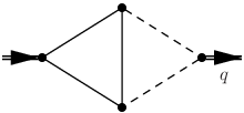
J(𝒟)​(𝐪2)=∫d𝒟​Δ​d𝒟​pπ𝒟​j​(𝐩,𝚫,𝐪)=∫π−𝒟​d𝒟​Δ​d𝒟​p𝚫2​(𝐪+𝚫)2​(𝐩2+1)​[(𝐩+𝐪)2+1]​[(𝐩−𝚫)2+1],J^{\left(\mathcal{D}\right)}\left(\mathbf{q}^{2}\right)=\int\frac{d^{\mathcal{D}}\Delta d^{\mathcal{D}}p}{\pi^{\mathcal{D}}}\,j\left(\mathbf{p},\boldsymbol{\Delta},\mathbf{q}\right)\\ =\int\frac{\pi^{-\mathcal{D}}d^{\mathcal{D}}\Delta d^{\mathcal{D}}p}{\mathbf{\Delta}^{2}\left(\mathbf{q}+\boldsymbol{\boldsymbol{\Delta}}\right)^{2}\left(\mathbf{p}^{2}+1\right)\left[\left(\mathbf{p}+\mathbf{q}\right)^{2}+1\right]\left[\left(\mathbf{p}-\boldsymbol{\boldsymbol{\Delta}}\right)^{2}+1\right]}, (7)

at 𝐪2≪1\mathbf{q}^{2}\ll 1. The corresponding diagram is depicted in Fig. 1.

Refer to caption
Figure 1: Example of the integral having nonanalytic expansion in qq.

The small-𝐪2\mathbf{q}^{2} expansion of this integral, obtained in Ref. [12], has the form:

J(𝒟)​(𝐪2)=∑n=0∞Cn​(𝒟)​(−𝐪2)n+(𝐪2)𝒟2−2​∑n=0∞Dn​(𝒟)​(−𝐪2)n,J^{\left(\mathcal{D}\right)}\left(\mathbf{q}^{2}\right)=\sum_{n=0}^{\infty}C_{n}\left(\mathcal{D}\right)\,\left(-\mathbf{q}^{2}\right)^{n}+\left(\mathbf{q}^{2}\right)^{\frac{\mathcal{D}}{2}-2}\sum_{n=0}^{\infty}D_{n}\left(\mathcal{D}\right)\,\left(-\mathbf{q}^{2}\right)^{n}\,, (8)
Cn​(𝒟)\displaystyle C_{n}\left(\mathcal{D}\right) =Γ⁡(n+3−𝒟/2)(n+3−𝒟/2)​(𝒟−3)[Γ(𝒟/2−1)Γ⁡(n+5−𝒟)​Γ​(n+3−𝒟/2)Γ⁡(n+𝒟/2)​Γ​(2​n+6−𝒟)\displaystyle=\frac{\Gamma\left(n+3-\mathcal{D}/2\right)}{\left(n+3-\mathcal{D}/2\right)\left(\mathcal{D}-3\right)}\left[\Gamma\left(\mathcal{D}/2-1\right)\frac{\Gamma\left(n+5-\mathcal{D}\right)\Gamma\left(n+3-\mathcal{D}/2\right)}{\Gamma\left(n+\mathcal{D}/2\right)\Gamma\left(2n+6-\mathcal{D}\right)}\right.
−Γ⁡(n+2)​Γ​(2−𝒟/2)Γ⁡(2​n+3)],\displaystyle\left.-\frac{\Gamma\left(n+2\right)\Gamma\left(2-\mathcal{D}/2\right)}{\Gamma\left(2n+3\right)}\right], (9)
Dn​(𝒟)=Γ⁡(2−𝒟/2)​Γ​(𝒟/2−1)2​Γ⁡(n+1)​Γ​(n+3−𝒟/2)Γ⁡(𝒟−2)​Γ​(2​n+3).D_{n}\left(\mathcal{D}\right)=\Gamma\left(2-\mathcal{D}/2\right)\Gamma\left(\mathcal{D}/2-1\right)^{2}\frac{\Gamma\left(n+1\right)\Gamma\left(n+3-\mathcal{D}/2\right)}{\Gamma(\mathcal{D}-2)\Gamma\left(2n+3\right)}\,. (10)

The representation (8) determines J(𝒟)​(𝐪2)J^{\left(\mathcal{D}\right)}\left(\mathbf{q}^{2}\right) at 0<𝐪2<4.0<\mathbf{q}^{2}<4. The limit 𝐪2→0\mathbf{q}^{2}\rightarrow 0 essentially depends on 𝒟\mathcal{D}. For 𝒟>4\mathcal{D}>4, this limit is equal to C0​(𝒟)C_{0}\left(\mathcal{D}\right) and can be considered as the value of the function J(𝒟)J^{\left(\mathcal{D}\right)} at 𝐪2=0.\mathbf{q}^{2}=0. For 𝒟<4\mathcal{D}<4, there is no finite 𝐪2→0\mathbf{q}^{2}\rightarrow 0 limit of the representation (8). However, the value J(𝒟)​(0)J^{\left(\mathcal{D}\right)}\left(0\right) defined via the analytic continuation with respect to 𝒟\mathcal{D} from the region 𝒟>4\mathcal{D}>4 is still C0​(𝒟).C_{0}\left(\mathcal{D}\right). In other words, the limit 𝐪2→0\mathbf{q}^{2}\rightarrow 0 is not commuting with the analytic continuation with respect to 𝒟\mathcal{D}. The same claim is valid for the derivatives of J(𝒟)​(𝐪2)J^{\left(\mathcal{D}\right)}\left(\mathbf{q}^{2}\right) with respect to 𝐪2\mathbf{q}^{2}. As a consequence, the integrand expanded in 𝐪\mathbf{q} gives only the terms ∝(𝐪2)n\propto\left(\mathbf{q}^{2}\right)^{n} after the integration within the dimensional regularization. These terms correspond to the first sum in the right-hand side of Eq. (8):

∫d𝒟​Δ​d𝒟​pπ𝒟​[∑n=0∞qi1​…​qinn!​∂nj⁡(𝐩,𝚫,𝐪)∂qi1​…​∂qin|𝐪=0]=∑n=0∞Cn​(𝒟)​(−𝐪24)n.\int\frac{d^{\mathcal{D}}\Delta\,d^{\mathcal{D}}p}{\pi^{\mathcal{D}}}\left[\sum_{n=0}^{\infty}\frac{q^{i_{1}}\ldots q^{i_{n}}}{n!}\left.\frac{\partial^{n}\,j\left(\mathbf{p},\boldsymbol{\Delta},\mathbf{q}\right)}{\partial q^{i_{1}}\ldots\partial q^{i_{n}}}\right|_{\mathbf{q}=0}\right]=\sum_{n=0}^{\infty}C_{n}\left(\mathcal{D}\right)\,\left(-\frac{\mathbf{q}^{2}}{4}\right)^{n}. (11)

Note that the expansion of the massless propagators is valid only in the region Δ≫q\Delta\gg q (hard region). In order to obtain the rest terms of the expansion (8) one has to determine the contribution of the region Δ∼q\Delta\sim q (soft region). To separate these contributions, we use the following trick. In the soft region the massive propagators can be expanded in both 𝐪\mathbf{q} and 𝚫\boldsymbol{\Delta}. Let us truncate this expansion at some fixed order NN in 𝐪\mathbf{q} and 𝚫\boldsymbol{\Delta}:

jsoft​(N,𝐩,𝚫,𝐪)\displaystyle j_{\mathrm{soft}}\left(N,\mathbf{p},\boldsymbol{\Delta},\mathbf{q}\right) =∑n=0Njsoft(n)​(𝐩,𝚫,𝐪),\displaystyle=\sum_{n=0}^{N}j_{\mathrm{soft}}^{(n)}\left(\mathbf{p},\boldsymbol{\Delta},\mathbf{q}\right), (12)
jsoft(n)​(𝐩,𝚫,𝐪)\displaystyle j_{\mathrm{soft}}^{(n)}\left(\mathbf{p},\boldsymbol{\Delta},\mathbf{q}\right) =∂nτ4​j​(𝐩,τ​𝚫,τ​𝐪)n!​∂τn|τ=0, so that ​jsoft(n)=O⁡(qn−4).\displaystyle=\left.\frac{\partial^{n}\tau^{4}j\left(\mathbf{p},\tau\boldsymbol{\Delta},\tau\mathbf{q}\right)}{n!\partial\tau^{n}}\right|_{\tau=0}\,,\text{ so that }j_{\mathrm{soft}}^{(n)}=O\left(q^{n-4}\right).

Now we can identically rewrite J(𝒟)​(𝐪2)J^{\left(\mathcal{D}\right)}\left(\mathbf{q}^{2}\right) as

J(𝒟)​(𝐪2)=Jhard(𝒟)​(𝐪2)+Jsoft(𝒟)​(𝐪2)\displaystyle J^{\left(\mathcal{D}\right)}\left(\mathbf{q}^{2}\right)=J_{\mathrm{hard}}^{\left(\mathcal{D}\right)}\left(\mathbf{q}^{2}\right)+J_{\mathrm{soft}}^{\left(\mathcal{D}\right)}\left(\mathbf{q}^{2}\right)
=∫d𝒟​Δ​d𝒟​pπ𝒟​[j⁡(𝐩,𝚫,𝐪)−jsoft​(N,𝐩,𝚫,𝐪)]+∫d𝒟​Δ​d𝒟​pπ𝒟​jsoft​(N,𝐩,𝚫,𝐪).\displaystyle=\int\frac{d^{\mathcal{D}}\Delta\,d^{\mathcal{D}}p}{\pi^{\mathcal{D}}}\,\left[j\left(\mathbf{p},\boldsymbol{\Delta},\mathbf{q}\right)-\,j_{\mathrm{soft}}\left(N,\mathbf{p},\boldsymbol{\Delta},\mathbf{q}\right)\right]+\int\frac{d^{\mathcal{D}}\Delta\,d^{\mathcal{D}}p}{\pi^{\mathcal{D}}}\,j_{\mathrm{soft}}\left(N,\mathbf{p},\boldsymbol{\Delta},\mathbf{q}\right). (13)

The contribution of the soft region in the first term in Eq. (13) is suppressed as q𝒟+N−3q^{\mathcal{D+}N-3}, thus the integral of the difference j⁡(𝐩,𝚫,𝐪)−jsoft​(N,𝐩,𝚫,𝐪)j\left(\mathbf{p},\boldsymbol{\Delta},\mathbf{q}\right)-\,j_{\mathrm{soft}}\left(N,\mathbf{p},\boldsymbol{\Delta},\mathbf{q}\right) is determined by the region Δ∼1≫q\Delta\sim 1\gg q up to O⁡(q2​⌊(𝒟+N−3)/2⌋)O\left(q^{2\left\lfloor\left(\mathcal{D+}N-3\right)/2\right\rfloor}\right) term. In fact, the expansion of jsoft​(N,𝐩,𝚫,𝐪)\,j_{\mathrm{soft}}\left(N,\mathbf{p},\boldsymbol{\Delta},\mathbf{q}\right) in 𝐪\mathbf{q} gives scaleless functions of 𝚫\boldsymbol{\Delta}, which vanish after the integration in the dimensional regularization. Finally, we have

J(𝒟)​(𝐪2)\displaystyle J^{\left(\mathcal{D}\right)}\left(\mathbf{q}^{2}\right) =Jhard(𝒟)​(𝐪2)+Jsoft(𝒟)​(𝐪2)\displaystyle=J_{\mathrm{hard}}^{\left(\mathcal{D}\right)}\left(\mathbf{q}^{2}\right)+J_{\mathrm{soft}}^{\left(\mathcal{D}\right)}\left(\mathbf{q}^{2}\right)
=∑n=0∞∫d𝒟​Δ​d𝒟​pπ𝒟​jhard(n)​(𝐩,𝚫,𝐪)+∑n=0∞∫d𝒟​Δ​d𝒟​pπ𝒟​jsoft(n)​(𝐩,𝚫,𝐪),\displaystyle=\sum_{n=0}^{\infty}\int\frac{d^{\mathcal{D}}\Delta\,d^{\mathcal{D}}p}{\pi^{\mathcal{D}}}\,j_{\mathrm{hard}}^{(n)}\left(\mathbf{p},\boldsymbol{\Delta},\mathbf{q}\right)+\sum_{n=0}^{\infty}\int\frac{d^{\mathcal{D}}\Delta\,d^{\mathcal{D}}p}{\pi^{\mathcal{D}}}\,j_{\mathrm{soft}}^{(n)}\left(\mathbf{p},\boldsymbol{\Delta},\mathbf{q}\right), (14)
jhard(n)​(𝐩,𝚫,𝐪)\displaystyle j_{\mathrm{hard}}^{(n)}\left(\mathbf{p},\boldsymbol{\Delta},\mathbf{q}\right) =∂nj⁡(𝐩,𝚫,τ​𝐪)n!​∂τn|τ=0,jsoft(n)​(𝐩,𝚫,𝐪)=∂nτ4​j​(𝐩,τ​𝚫,τ​𝐪)n!​∂τn|τ=0.\displaystyle=\left.\frac{\partial^{n}j\left(\mathbf{p},\boldsymbol{\Delta},\tau\mathbf{q}\right)}{n!\partial\tau^{n}}\right|_{\tau=0},~j_{\mathrm{soft}}^{(n)}\left(\mathbf{p},\boldsymbol{\Delta},\mathbf{q}\right)=\left.\frac{\partial^{n}\tau^{4}j\left(\mathbf{p},\tau\boldsymbol{\Delta},\tau\mathbf{q}\right)}{n!\partial\tau^{n}}\right|_{\tau=0}.

Let us now use this approach for the calculation of the low-energy expansion of the polarization operator in the Coulomb field.

Refer to caption
Figure 2: The (Z​α)N(Z\alpha)^{N} contribution to the polarization operator. Solid lines denote the electron propagator, dashed lines denote the Coulomb field.

The (Z​α)N(Z\alpha)^{N} contribution (NN is even) is determined by the NN-loop diagrams depicted in Fig.  2. In the dimensional regularization, it can be represented in the form

Π(Z​α)Nμ​ν​(ω,𝐤,𝐪)=∫d​ε​d𝒟​p(2​π)𝒟+1​∏i=1N−1d𝒟​Δi(2​π)(N−1)​𝒟​𝔓μ​ν​(ε,𝐩,𝚫1,…​𝚫N−1,ω,𝐤,𝐪).\Pi_{(Z\alpha)^{N}}^{\mu\nu}\left(\omega,\mathbf{k},\mathbf{q}\right)=\int\frac{d\varepsilon\,d^{\mathcal{D}}p}{\left(2\pi\right)^{\mathcal{D}+1}}\frac{\prod_{i=1}^{N-1}d^{\mathcal{D}}\Delta_{i}}{\left(2\pi\right)^{\left(N-1\right)\mathcal{D}}}\,\mathfrak{P}^{\mu\nu}\left(\varepsilon,\mathbf{p},\boldsymbol{\Delta}_{1},\ldots\boldsymbol{\Delta}_{N-1},\omega,\mathbf{k},\mathbf{q}\right). (15)

Similar to the previous example, there are two different region of integration

hard region, when ε∼pi∼Δ1..N−1i∼m,\displaystyle\varepsilon\sim p^{i}\sim\Delta_{1..N-1}^{i}\sim m, (16)
soft region, when {ε∼pi∼m,Δ1..N−1i∼λ​m.\displaystyle\left\{\begin{array}[c]{rl}\varepsilon\sim p^{i}&\sim m,\\ \Delta_{1..N-1}^{i}&\sim\lambda\,m.\end{array}\right.

Again, the expansion of the polarization operator is the sum of the integrals of the expansion of the integrand in hard and soft regions. In the coordinate representation, these regions have a simple physical meaning. The characteristic size of the electron field fluctuations (the size of the electron loop) is of the order 1/m1/m. Hard region corresponds to the configurations where the distance between the Coulomb source and the electron loop is of the order of 1/m1/m. Soft region corresponds to the creation of the virtual electron-positron pair far from the Coulomb source. Obviously, there is no contribution from the region where only some of the momenta 𝚫n\boldsymbol{\Delta}_{n} are hard while the rest are soft. In the momentum representation, these regions correspond to massless tadpole diagrams which are zero in the dimensional regularization. Thus, the expansion of the polarization operator (15) has the form

Π(Z​α)Nμ​ν​(ω,𝐤,𝐪)=Π(Z​α)N,hardμ​ν​(ω,𝐤,𝐪)+Π(Z​α)N,softμ​ν​(ω,𝐤,𝐪)=∑n∫d​ε​d𝒟​p(2​π)𝒟+1​∏i=1N−1d𝒟​Δi(2​π)(N−1)​𝒟​𝔓hardμ​ν​(n)+∑n∫d​ε​d𝒟​p(2​π)𝒟+1​∏i=1N−1d𝒟​Δi(2​π)(N−1)​𝒟​𝔓softμ​ν​(n),\Pi_{(Z\alpha)^{N}}^{\mu\nu}\left(\omega,\mathbf{k},\mathbf{q}\right)=\Pi_{(Z\alpha)^{N},\text{hard}}^{\mu\nu}\left(\omega,\mathbf{k},\mathbf{q}\right)+\Pi_{(Z\alpha)^{N},\text{soft}}^{\mu\nu}\left(\omega,\mathbf{k},\mathbf{q}\right)\\ =\sum_{n}\int\frac{d\varepsilon\,d^{\mathcal{D}}p}{\left(2\pi\right)^{\mathcal{D}+1}}\frac{\prod_{i=1}^{N-1}d^{\mathcal{D}}\Delta_{i}}{\left(2\pi\right)^{\left(N-1\right)\mathcal{D}}}\,\mathfrak{P}_{\text{hard}}^{\mu\nu\left(n\right)}+\sum_{n}\int\frac{d\varepsilon\,d^{\mathcal{D}}p}{\left(2\pi\right)^{\mathcal{D}+1}}\frac{\prod_{i=1}^{N-1}d^{\mathcal{D}}\Delta_{i}}{\left(2\pi\right)^{\left(N-1\right)\mathcal{D}}}\,\mathfrak{P}_{\text{soft}}^{\mu\nu\left(n\right)}, (19)
𝔓hardμ​ν​(n)\displaystyle\mathfrak{P}_{\text{hard}}^{\mu\nu\left(n\right)} =∂n𝔓μ​ν​(ε,𝐩,𝚫1,…​𝚫N−1,τ​ω,τ​𝐤,τ​𝐪)n!​∂τn|τ=0,\displaystyle=\left.\frac{\partial^{n}\mathfrak{P}^{\mu\nu}\left(\varepsilon,\mathbf{p},\boldsymbol{\Delta}_{1},\ldots\boldsymbol{\Delta}_{N-1},\tau\omega,\tau\mathbf{k},\tau\mathbf{q}\right)}{n!\partial\tau^{n}}\right|_{\tau=0}, (20)
𝔓softμ​ν​(n)\displaystyle\mathfrak{P}_{\text{soft}}^{\mu\nu\left(n\right)} =∂nτN−2​𝔓μ​ν​(ε,𝐩,τ​𝚫1,…​τ​𝚫N−1,τ​ω,τ​𝐤,τ​𝐪)n!​∂τn|τ=0.\displaystyle=\left.\frac{\partial^{n}\tau^{N-2}\mathfrak{P}^{\mu\nu}\left(\varepsilon,\mathbf{p},\tau\boldsymbol{\Delta}_{1},\ldots\tau\boldsymbol{\Delta}_{N-1},\tau\omega,\tau\mathbf{k},\tau\mathbf{q}\right)}{n!\partial\tau^{n}}\right|_{\tau=0}. (21)

Note that the simple power counting allows one to estimate the leading terms of the hard and soft contribution as

Π(Z​α)N,hardμ​ν​(ω,𝐤,𝐪)\displaystyle\Pi_{(Z\alpha)^{N},\text{hard}}^{\mu\nu}\left(\omega,\mathbf{k},\mathbf{q}\right) ∼λ2,\displaystyle\sim\lambda^{2},
Π(Z​α)N,softμ​ν​(ω,𝐤,𝐪)\displaystyle\Pi_{(Z\alpha)^{N},\text{soft}}^{\mu\nu}\left(\omega,\mathbf{k},\mathbf{q}\right) ∼λ(N−1)​(𝒟−1)+1.\displaystyle\sim\lambda^{\left(N-1\right)\left(\mathcal{D}-1\right)+1}. (22)

Using Eq. (19), one can calculate the contributions of the hard and soft regions separately.

3 Method of calculation

Refer to caption
Figure 3: Graphical representation of the soft contribution.

The contribution of the soft region can be graphically represented as the tree diagram shown in Fig. 3. The local multiphoton vertex depicted as a thick dot corresponds to the expansion of the fermionic loop with respect to the soft momenta 𝚫i,k,q\boldsymbol{\Delta}_{i},k,q. The expansion is expressed via the integrals of the following form

∫d​ε​d𝒟​p(2​π)𝒟+1​(ε2−𝐩2−m2+i​0)−n=i​(−1)n​Γ​(n−𝒟/2−1/2)(4​π)(𝒟+1)/2​Γ​(n)​m2​n−𝒟−1.\int\frac{d\varepsilon\,d^{\mathcal{D}}p}{\left(2\pi\right)^{\mathcal{D}+1}}\left(\varepsilon^{2}-\mathbf{p}^{2}-m^{2}+i0\right)^{-n}=\frac{i\left(-1\right)^{n}\Gamma\left(n-\mathcal{D}/2-1/2\right)}{\left(4\pi\right)^{\left(\mathcal{D}+1\right)/2}\Gamma\left(n\right)m^{2n-\mathcal{D}-1}}\,. (23)

The remaining integrals over 𝚫i\boldsymbol{\Delta}_{i} can be easily evaluated in the coordinate representation. Naturally, the contribution of the soft region can be calculated also with the help of the derivative expansion of the one-loop effective QED action.

The contribution of the hard region determined by Eq. (19) is expressed in terms of the NN-loop tadpoles. In particular, in (Z​α)2\left(Z\alpha\right)^{2} order, the basic integral has the following form

I=∫d​ε​d𝒟​p​d𝒟​Δ(2​π)2​𝒟+1​1(ε2−𝐩2−m2+i​0)n1​(ε2−(𝐩−𝚫)2−m2+i​0)n2​(𝚫2)n3.I=\int\frac{d\varepsilon\,d^{\mathcal{D}}p\,d^{\mathcal{D}}\Delta}{\left(2\pi\right)^{2\mathcal{D}+1}}\frac{1}{\left(\varepsilon^{2}-\mathbf{p}^{2}-m^{2}+i0\right)^{n_{1}}\left(\varepsilon^{2}-\left(\mathbf{p-}\boldsymbol{\Delta}\right)^{2}-m^{2}+i0\right)^{n_{2}}\left(\boldsymbol{\Delta}^{2}\right)^{n_{3}}}. (24)

After the Wick rotation ε→i​ε\varepsilon\rightarrow i\varepsilon and rescaling 𝐩→ε2+m2​𝐩,𝚫→ε2+m2​𝚫\mathbf{p}\rightarrow\sqrt{\varepsilon^{2}+m^{2}}\mathbf{p},\mathbf{~}\boldsymbol{\Delta}\rightarrow\sqrt{\varepsilon^{2}+m^{2}}\boldsymbol{\Delta}, we integrate over ε\varepsilon and obtain

I\displaystyle I =i​m1−2​γ​Γ​(γ−1/2)2​π​Γ​(γ)​∫d𝒟​p​d𝒟​Δ(2​π)2​𝒟​(−1)n1+n2(𝐩2+1)n1​((𝐩−𝚫)2+1)n2​(𝚫2)n3,\displaystyle=i\frac{m^{1-2\gamma}\Gamma\left(\gamma-1/2\right)}{2\sqrt{\pi}\,\Gamma\left(\gamma\right)}\int\frac{d^{\mathcal{D}}p\,d^{\mathcal{D}}\Delta}{\left(2\pi\right)^{2\mathcal{D}}}\frac{\left(-1\right)^{n_{1}+n_{2}}}{\left(\mathbf{p}^{2}+1\right)^{n_{1}}\left(\left(\mathbf{p-}\boldsymbol{\Delta}\right)^{2}+1\right)^{n_{2}}\left(\boldsymbol{\Delta}^{2}\right)^{n_{3}}}, (25)
γ\displaystyle\gamma =n1+n2+n3−𝒟.\displaystyle=n_{1}+n_{2}+n_{3}-\mathcal{D}.

The remaining integral is the two-loop tadpole in 𝒟=3+ϵ\mathcal{D}=3+\epsilon dimensions which can be easily expressed in terms of Γ\Gamma-functions.

Performing the similar integration over ε\varepsilon in (Z​α)4\left(Z\alpha\right)^{4} order, we express the contribution of the hard region in terms of the integrals of the topology (and its subtopologies) depicted in Fig. 4.

Refer to caption
Figure 4: Topology of the integrals required for the calculation of the low-energy expansion of the polarization operator in (Z​α)4\left(Z\alpha\right)^{4} order.

The general form of such integral is

Jn1​…​n10=∫d𝒟​k1​d𝒟​k2​d𝒟​k3​d𝒟​k4​D9−n9​D10−n10π2​𝒟​D1n1​D2n2​D3n3​D4n4​D5n5​D6n6​D7n7​D8n8,J_{n_{1}\ldots n_{10}}=\int\frac{d^{\mathcal{D}}k_{1}d^{\mathcal{D}}k_{2}d^{\mathcal{D}}k_{3}d^{\mathcal{D}}k_{4}D_{9}^{-n_{9}}D_{10}^{-n_{10}}}{\pi^{2\mathcal{D}}D_{1}^{n_{1}}D_{2}^{n_{2}}D_{3}^{n_{3}}D_{4}^{n_{4}}D_{5}^{n_{5}}D_{6}^{n_{6}}D_{7}^{n_{7}}D_{8}^{n_{8}}}, (26)

where

D1,…,4=k1,…,42+1,\displaystyle D_{1,\ldots,4}=k_{1,\ldots,4}^{2}+1,\qquad\ (27)
D5=(k1−k2)2,D6=(k2−k3)2,\displaystyle D_{5}=\left(k_{1}-k_{2}\right)^{2},\quad D_{6}=\left(k_{2}-k_{3}\right)^{2},
D7=(k3−k4)2,D8=(k4−k1)2,\displaystyle D_{7}=\left(k_{3}-k_{4}\right)^{2},\quad D_{8}=\left(k_{4}-k_{1}\right)^{2},
D9=(k1−k3)2,D10=(k2−k4)2.\displaystyle D_{9}=\left(k_{1}-k_{3}\right)^{2},\quad D_{10}=\left(k_{2}-k_{4}\right)^{2}.

The IBP reduction procedure [13, 14] allows one to express any vacuum integral of the considered topology via the five master integrals shown in Fig. 5.

Refer to caption
(a) jCakej_{\text{Cake}}
Refer to caption
(b) jInfinityj_{\text{Infinity}}
Refer to caption
(c) jMelonj_{\text{Melon}}
Refer to caption
(d) jTumblerj_{\text{Tumbler}}
Refer to caption
(e) jCloverj_{\text{Clover}}
Figure 5: Master integrals of the topology, shown in Fig. 4.

On these diagrams the solid and dashed lines denote the massive (k2+1)−1\left(k^{2}+1\right)^{-1} and massless (k2)−1\left(k^{2}\right)^{-1} propagators. For each loop momentum the integration measure is taken as

d𝒟​kπ𝒟/2.\frac{d^{\mathcal{D}}k}{\pi^{\mathcal{D}/2}}.

Four of these integrals are trivially expressed in terms of Γ\Gamma-functions. Their explicit forms are presented in Appendix. The only nontrivial master integral is JCakeJ_{\text{Cake}}. After the IBP reduction, the master integral JCakeJ_{\text{Cake}} enters the polarization operator with the coefficient, having the first-order pole in the point 𝒟=3\mathcal{D}=3. Therefore, we need to determine the O⁡(ϵ0)O\left(\epsilon^{0}\right) and O⁡(ϵ1)O\left(\epsilon^{1}\right) terms of the expansion of JCakeJ_{\text{Cake}}.

We find it convenient to use the recurrence relation with respect to space-time dimension, see Ref. [15]. First, we use the Feynman parameterization to obtain the relation

JCake(𝒟−2)​≡d​e​f​J1111111100(𝒟−2)\displaystyle J_{\text{Cake}}^{(\mathcal{D}-2)}\overset{def}{\equiv}J_{1111111100}^{(\mathcal{D}-2)} =8​J1112122200(𝒟)+8​J1112221200(𝒟)+8​J1122211200(𝒟)+8​J1222111200(𝒟)\displaystyle=8J_{1112122200}^{(\mathcal{D})}+8J_{1112221200}^{(\mathcal{D})}+8J_{1122211200}^{(\mathcal{D})}+8J_{1222111200}^{(\mathcal{D})}
+4​J1122121200(𝒟)+4​J1212112200(𝒟)+4​J1212121200(𝒟)+J2222111100(𝒟).\displaystyle+4J_{1122121200}^{(\mathcal{D})}+4J_{1212112200}^{(\mathcal{D})}+4J_{1212121200}^{(\mathcal{D})}+J_{2222111100}^{(\mathcal{D})}. (28)

Then, using the IBP identities, we express the integrals in the right-hand side of this relation via the five master integrals from Fig. 5. In particular, the last term in Eq. (28) can be expressed via the master integrals as follows

J2(5+ϵ)​≡d​e​f​J2222111100(5+ϵ)\displaystyle J_{2}^{(5+\epsilon)}\overset{def}{\equiv}J_{2222111100}^{(5+\epsilon)} =aCake​JCake(5+ϵ)+aCloverϵ3​JClover(5+ϵ)\displaystyle=a_{\text{Cake}}J_{\text{Cake}}^{(5+\epsilon)}+\frac{a_{\text{Clover}}}{\epsilon^{3}}J_{\text{Clover}}^{(5+\epsilon)}
+aInfinity​JInfinity(5+ϵ)+aTumblerϵ2​JTumbler(5+ϵ)+aMelonϵ2​JMelon(5+ϵ).\displaystyle+a_{\text{Infinity}}J_{\text{Infinity}}^{(5+\epsilon)}+\frac{a_{\text{Tumbler}}}{\epsilon^{2}}J_{\text{Tumbler}}^{(5+\epsilon)}+\frac{a_{\text{Melon}}}{\epsilon^{2}}J_{\text{Melon}}^{(5+\epsilon)}\,. (29)

The coefficients aia_{i} are presented in the Appendix. They are chosen to be finite in the limit ϵ→0\epsilon\rightarrow 0. After the reduction, we have the following recurrence relation:

JCake(3+ϵ)=ϵ​bCake​JCake(5+ϵ)+bCloverϵ2​JClover(5+ϵ)+bInfinity​JInfinity(5+ϵ)+bTumblerϵ​JTumbler(5+ϵ)+bMelonϵ​JMelon(5+ϵ).J_{\text{Cake}}^{(3+\epsilon)}=\epsilon b_{\text{Cake}}J_{\text{Cake}}^{(5+\epsilon)}+\frac{b_{\text{Clover}}}{\epsilon^{2}}\,J_{\text{Clover}}^{(5+\epsilon)}\\ +b_{\text{Infinity}}J_{\text{Infinity}}^{(5+\epsilon)}+\frac{b_{\text{Tumbler}}}{\epsilon}\,J_{\text{Tumbler}}^{(5+\epsilon)}+\frac{b_{\text{Melon}}}{\epsilon}\,J_{\text{Melon}}^{(5+\epsilon)}\,. (30)

Again, the coefficients bib_{i} are chosen to be finite in the limit ϵ→0\epsilon\rightarrow 0 and are presented in the Appendix. Now we use the following trick. Let us express JCake(5+ϵ)J_{\text{Cake}}^{(5+\epsilon)} from Eq. (29) and substitute into Eq.  (28). We obtain

JCake(3+ϵ)=ϵ​bCakeaCake​J2(5+ϵ)+bCakeϵ2​(bCloverbCake−aCloveraCake)​JClover(5+ϵ)+bCake​(bInfinitybCake−ϵ​aInfinityaCake)​JInfinity(5+ϵ)+bCakeϵ​(bTumblerbCake−aTumbleraCake)​JTumbler(5+ϵ)+bCakeϵ​(bMelonbCake−aMelonaCake)​JMelon(5+ϵ).J_{\text{Cake}}^{(3+\epsilon)}=\frac{\epsilon b_{\text{Cake}}}{a_{\text{Cake}}}\,J_{2}^{(5+\epsilon)}+\frac{b_{\text{Cake}}}{\epsilon^{2}}\left(\frac{b_{\text{Clover}}}{b_{\text{Cake}}}-\frac{a_{\text{Clover}}}{a_{\text{Cake}}}\right)J_{\text{Clover}}^{(5+\epsilon)}\\ +b_{\text{Cake}}\left(\frac{b_{\text{Infinity}}}{b_{\text{Cake}}}-\frac{\epsilon\,a_{\text{Infinity}}}{a_{\text{Cake}}}\right)J_{\text{Infinity}}^{(5+\epsilon)}+\frac{b_{\text{Cake}}}{\epsilon}\left(\frac{b_{\text{Tumbler}}}{b_{\text{Cake}}}\,-\frac{a_{\text{Tumbler}}}{a_{\text{Cake}}}\right)J_{\text{Tumbler}}^{(5+\epsilon)}\\ +\frac{b_{\text{Cake}}}{\epsilon}\left(\frac{b_{\text{Melon}}}{b_{\text{Cake}}}-\frac{a_{\text{Melon}}}{a_{\text{Cake}}}\right)J_{\text{Melon}}^{(5+\epsilon)}\,. (31)

Since the integral J2(𝒟)J_{2}^{\left(\mathcal{D}\right)} is finite in 𝒟=5\mathcal{D}=5 and the coefficient in front of this integral in Eq. (31) contains ϵ\epsilon factor, the first term in the right-hand side of Eq. (31) does not contribute in ϵ0\epsilon^{0} order. Expanding the coefficient ai,bia_{i},b_{i} and the four simple master integrals, we obtain

JCake(3+ϵ)=π46+ϵ⁡[π43​(C−ln⁡2−118)−π2−34​J2(5)]+O⁡(ϵ2),J_{\text{Cake}}^{(3+\epsilon)}=\frac{\pi^{4}}{6}+\epsilon\left[\frac{\pi^{4}}{3}\left(C-\ln 2-\frac{11}{8}\right)-\pi^{2}-\frac{3}{4}\,J_{2}^{(5)}\right]+O\left(\epsilon^{2}\right)\,, (32)

where C=0.577​…C=0.577... is the Euler constant. Note, that using this trick we have obtained the O⁡(ϵ0)O\left(\epsilon^{0}\right) term of JCake(3+ϵ)J_{\text{Cake}}^{(3+\epsilon)} “for free”.

In order to calculate the O⁡(ϵ)O\left(\epsilon\right) term, let us consider the general solution of the recurrence (28). Taking into account the explicit form of the coefficient bCakeb_{\text{Cake}}, we obtain

JCake(𝒟)=J0​(𝒟)​[P⁡(𝒟)+∑i=14∑n=1∞ci(𝒟+2​n)J0​(𝒟+2​n)​Ji(𝒟+2​n)],J_{\text{Cake}}^{(\mathcal{D})}=J_{0}\left(\mathcal{D}\right)\left[P\left(\mathcal{D}\right)+\sum_{i=1}^{4}\sum_{n=1}^{\infty}\frac{c_{i}^{(\mathcal{D}+2n)}}{J_{0}(\mathcal{D}+2n)}J_{i}^{(\mathcal{D}+2n)}\right], (33)

where

J0​(𝒟)\displaystyle J_{0}\left(\mathcal{D}\right) =23​𝒟​Γ​(1−𝒟/2)​Γ​(3​𝒟/2−11/2)Γ⁡(𝒟−2)​Γ​(𝒟−3)2,\displaystyle=\frac{2^{3\mathcal{D}}\Gamma\left(1-\mathcal{D}/2\right)\Gamma\left(3\mathcal{D}/2-11/2\right)}{\Gamma(\mathcal{D}-2)\Gamma(\mathcal{D}-3)^{2}}, (34)
cClover\displaystyle c_{\text{Clover}} =bCloverϵ3​bCake,cInfinity=bInfinityϵ​bCake,\displaystyle=\frac{b_{\text{Clover}}}{\epsilon^{3}b_{\text{Cake}}}\ ,\quad c_{\text{Infinity}}=\frac{b_{\text{Infinity}}}{\epsilon b_{\text{Cake}}},
cTumbler\displaystyle c_{\text{Tumbler}} =bTumblerϵ2​bCake,cMelon=bMelonϵ2​bCake,\displaystyle=\frac{b_{\text{Tumbler}}}{\epsilon^{2}b_{\text{Cake}}}\ ,\quad c_{\text{Melon}}=\frac{b_{\text{Melon}}}{\epsilon^{2}b_{\text{Cake}}},

and P⁡(𝒟)=P⁡(𝒟+2)P\left(\mathcal{D}\right)=P\left(\mathcal{D}+2\right) is a periodic function of 𝒟\mathcal{D}. Note that, using the explicit form of the simple master integrals, Eq. (62), the sums in Eq. (33) can be checked to converge rapidly. In order to fix the function P⁡(𝒟)P\left(\mathcal{D}\right), we have to calculate the leading asymptotic of JCake(𝒟)J_{\text{Cake}}^{(\mathcal{D})} at 𝒟→+∞\mathcal{D}\rightarrow+\infty. However, the calculation of this asymptotic is not a simple problem. Instead, we may proceed in the alternative way by applying the method of difference equations described in Ref. [16]. According to this method, we derive the recurrence relation in xx for Jx​111111100(𝒟)J_{x111111100}^{(\mathcal{D})}:

Jx​111111100(𝒟)\displaystyle J_{x111111100}^{(\mathcal{D})} =C⁡(x)​Jx+1,111111100(𝒟)+F⁡(x),\displaystyle=C(x)J_{x+1,111111100}^{(\mathcal{D})}+F(x), (35)
C⁡(x)\displaystyle C(x) =x⁡(x+11−3​𝒟)(x+5−3​𝒟/2)​(x+3−𝒟),\displaystyle=\frac{x\left(x+11-3\mathcal{D}\right)}{\left(x+5-3\mathcal{D}/2\right)\left(x+3-\mathcal{D}\right)}\,, (36)

where F⁡(x)F(x) is expressed in terms of finite sums of Γ\Gamma- functions. The solution of this relation is

Jx​111111100(𝒟)\displaystyle J_{x111111100}^{(\mathcal{D})} =G(𝒟)​(x)​[R(𝒟)​(x)+∑y=x∞F⁡(y)G⁡(y)],\displaystyle=G^{(\mathcal{D})}\left(x\right)\left[R^{(\mathcal{D})}\left(x\right)+\sum_{y=x}^{\infty}\frac{F(y)}{G\left(y\right)}\right], (37)
G(𝒟)​(x)\displaystyle G^{(\mathcal{D})}\left(x\right) =Γ⁡(x+5−3​𝒟/2)​Γ​(x+3−𝒟)Γ⁡(x)​Γ​(x+11−3​𝒟),\displaystyle=\frac{\Gamma\left(x+5-3\mathcal{D}/2\right)\Gamma\left(x+3-\mathcal{D}\right)}{\Gamma\left(x\right)\Gamma\left(x+11-3\mathcal{D}\right)}, (38)

where R(𝒟)​(x)R^{(\mathcal{D})}\left(x\right) is a periodic function of xx, which can be determined through the Jx​111111100(𝒟)J_{x111111100}^{(\mathcal{D})} asymptotic behaviour in x→∞x\rightarrow\infty limit. At large xx, the xx-dependence of Jx​111111100(𝒟)J_{x111111100}^{(\mathcal{D})} factorizes into ∫d𝒟​k1​(k12+1)−x\int d^{\mathcal{D}}k_{1}\,\left(k_{1}^{2}+1\right)^{-x}. Using the large-xx behaviour of the function G(𝒟)​(x)G^{(\mathcal{D})}\left(x\right), we find

Jx​111111100(𝒟)G(𝒟)​(x)|x→∞∼x3−𝒟.\left.\frac{J_{x111111100}^{(\mathcal{D})}}{G^{(\mathcal{D})}\left(x\right)}\right|_{x\rightarrow\infty}\sim x^{3-\mathcal{D}}. (39)

Therefore, for 𝒟>3\mathcal{D}>3 we have R⁡(x)=0R\left(x\right)=0 and we can use Eq. (37) to estimate numerically the function P⁡(𝒟)P\left(\mathcal{D}\right) in Eq. (33). It should be noted that the recurrence relation (35) can be hardly applied near 𝒟=3\mathcal{D}=3 due to the slow convergence of the sum in the right-hand side of Eq. (37). Performing the estimation of P⁡(𝒟)P\left(\mathcal{D}\right) for several non-integer values of 𝒟\mathcal{D}, we find that in all cases the value of the function P⁡(𝒟)P\left(\mathcal{D}\right) is compatible with zero up to 10−1010^{-10}. Thus, our ansatz is P⁡(𝒟)=0P\left(\mathcal{D}\right)=0, and we have

JCake(3+ϵ)=8ϵ+3​Γ​(−ϵ2−12)​Γ​(3​ϵ2−1)ϵ​Γ​(ϵ)3​∑n=0∞T⁡(2​n+ϵ),J_{\text{Cake}}^{(3+\epsilon)}=\frac{8^{\epsilon+3}\Gamma\left(-\frac{\epsilon}{2}-\frac{1}{2}\right)\Gamma\left(\frac{3\epsilon}{2}-1\right)}{\epsilon\Gamma(\epsilon)^{3}}\sum_{n=0}^{\infty}T\left(2n+\epsilon\right), (40)
T⁡(ν)\displaystyle T\left(\nu\right) =8−ν−5​(ν+1)​(14​ν3+40​ν2+35​ν+10)​Γ​(−ν2−12)3​Γ​(ν)3Γ⁡(32​ν+2)\displaystyle=\frac{8^{-\nu-5}(\nu+1)\left(14\nu^{3}+40\nu^{2}+35\nu+10\right)\Gamma\left(-\frac{\nu}{2}-\frac{1}{2}\right)^{3}\Gamma(\nu)^{3}}{\Gamma\left(\frac{3}{2}\nu+2\right)}
−π7/2​(6417​ν5+13266​ν4+8368​ν3+980​ν2−585​ν−126)​Γ​(ν)6144​ν​(3​ν−1)​(3​ν+1)​Γ​(−2​ν)​Γ​(3​ν+4)​cos⁡(π​ν2)​sin2⁡(π​ν)​cos⁡(3​π​ν2)\displaystyle-\frac{\pi^{7/2}\left(6417\nu^{5}+13266\nu^{4}+8368\nu^{3}+980\nu^{2}-585\nu-126\right)\Gamma(\nu)}{6144\nu(3\nu-1)(3\nu+1)\Gamma(-2\nu)\Gamma(3\nu+4)\cos\left(\frac{\pi\nu}{2}\right)\sin^{2}(\pi\nu)\cos\left(\frac{3\pi\nu}{2}\right)}
+π5/2​(585​ν3+372​ν2+7​ν−12)​Γ​(ν)​Γ​(ν+12)2​tan⁡(3​π​ν2)12288​(3​ν−1)​(3​ν+1)​Γ​(2​ν+2)​cos⁡(π​ν2)​sin⁡(2​π​ν)\displaystyle+\frac{\pi^{5/2}\left(585\nu^{3}+372\nu^{2}+7\nu-12\right)\Gamma(\nu)\Gamma\left(\frac{\nu+1}{2}\right)^{2}\tan\left(\frac{3\pi\nu}{2}\right)}{12288(3\nu-1)(3\nu+1)\Gamma(2\nu+2)\cos\left(\frac{\pi\nu}{2}\right)\sin\left(2\pi\nu\right)}
−π3/2​(3897​ν4+3870​ν3+797​ν2−198​ν−54)​Γ​(ν)2​Γ​(ν+12)3​tan⁡(3​π​ν2)36864​(3​ν−1)​(3​ν+1)​Γ​(2​ν+2)​Γ​(32​ν+32)​sin⁡(2​π​ν)​sin⁡(π​ν2).\displaystyle-\frac{\pi^{3/2}\left(3897\nu^{4}+3870\nu^{3}+797\nu^{2}-198\nu-54\right)\Gamma(\nu)^{2}\Gamma\left(\frac{\nu+1}{2}\right)^{3}\tan\left(\frac{3\pi\nu}{2}\right)}{36864(3\nu-1)(3\nu+1)\Gamma(2\nu+2)\Gamma\left(\frac{3}{2}\nu+\frac{3}{2}\right)\sin\left(2\pi\nu\right)\sin\left(\frac{\pi\nu}{2}\right)}\,. (41)

The series in this representation are converging rapidly. The first term in T⁡(ν)T\left(\nu\right), the most slowly decreasing one, behaves as 3−3​n3^{-3n}. Thus, roughly speaking, each two consecutive terms in the sum give three more decimal digits of precision. We claim this expression to be valid for arbitrary ϵ\epsilon. For example, one can easily reproduce terms of the expansion of JCakeJ_{\text{Cake}} near 𝒟=4\mathcal{D}=4 obtained in [17].

Using Eqs. (29), (40), we obtain

J2(5)\displaystyle J_{2}^{(5)} =−181​π2​(63​π2−488−72​ζ3)+∑n=1∞T2​(n),\displaystyle=-\frac{1}{81}\pi^{2}\left(63\pi^{2}-488-72\zeta_{3}\right)+\sum_{n=1}^{\infty}T_{2}(n)\,, (42)
T2​(n)\displaystyle T_{2}(n) =(−1)n​(56​n3+80​n2+35​n+5)​π2​((n−1)!)318​(2​n+1)2​(3​n+1)!\displaystyle=\frac{(-1)^{n}\left(56n^{3}+80n^{2}+35n+5\right)\pi^{2}((n-1)!)^{3}}{18(2n+1)^{2}(3n+1)!}
−(−1)n​2−4​n−1​(2340​n3+744​n2+7​n−6)​π4​((2​n)!)39​n​(36​n2−1)​(n!)2​(4​n+1)!\displaystyle-\frac{(-1)^{n}2^{-4n-1}\left(2340n^{3}+744n^{2}+7n-6\right)\pi^{4}((2n)!)^{3}}{9n\left(36n^{2}-1\right)(n!)^{2}(4n+1)!}
−16​π2​(2​n−1)!​(4​n−1)!27​(36​n2−1)2​(6​n+3)!\displaystyle-\frac{16\pi^{2}(2n-1)!(4n-1)!}{27\left(36n^{2}-1\right)^{2}(6n+3)!}
×(11088576​n6+7641216​n5+691632​n4−424512​n3−79356​n2+616​n+585)\displaystyle\times\left(11088576n^{6}+7641216n^{5}+691632n^{4}-424512n^{3}-79356n^{2}+616n+585\right)
+2​(−1)n​π2​((2​n)!)5​(3​n)!27​n2​(36​n2−1)2​(n!)3​(4​n+2)!​(6​n+1)!\displaystyle+\frac{2(-1)^{n}\pi^{2}((2n)!)^{5}(3n)!}{27n^{2}\left(36n^{2}-1\right)^{2}(n!)^{3}(4n+2)!(6n+1)!}
×(4489344​n6+2794176​n5+206352​n4−146880​n3−26032​n2−28​n+153)\displaystyle\times\left(4489344n^{6}+2794176n^{5}+206352n^{4}-146880n^{3}-26032n^{2}-28n+153\right)
−4​π2​(2​n)!​(4​n)!​(H2​n−1+2​H4​n−1−3​H6​n+3)27​n2​(36​n2−1)​(6​n+3)!\displaystyle-\frac{4\pi^{2}(2n)!(4n)!\left(H_{2n-1}+2H_{4n-1}-3H_{6n+3}\right)}{27n^{2}\left(36n^{2}-1\right)(6n+3)!}
×(102672​n5+106128​n4+33472​n3+1960​n2−585​n−63)\displaystyle\times\left(102672n^{5}+106128n^{4}+33472n^{3}+1960n^{2}-585n-63\right)
−(−1)n​π2​((2​n)!)5​(3​n)!​(3​Hn−1−10​H2​n−1−3​H3​n+1+4​H4​n+2+6​H6​n+3)54​n2​(36​n2−1)​(n!)3​(4​n+1)!​(6​n+1)!\displaystyle-\frac{(-1)^{n}\pi^{2}((2n)!)^{5}(3n)!\left(3H_{n-1}-10H_{2n-1}-3H_{3n+1}+4H_{4n+2}+6H_{6n+3}\right)}{54n^{2}\left(36n^{2}-1\right)(n!)^{3}(4n+1)!(6n+1)!}
×(31176​n4+15480​n3+1594​n2−198​n−27),\displaystyle\times\left(31176n^{4}+15480n^{3}+1594n^{2}-198n-27\right)\,,
J2(5)=0.0516516357945​….J_{2}^{(5)}=0.0516516357945\ldots. (43)

Here Hn=∑k=1nk−1H_{n}=\sum_{k=1}^{n}k^{-1} is a harmonic number. Unfortunately, we have not been able to express the sums in Eq. (42) in terms of ζ\zeta-functions and alike. However, the numerical convergence of the above series is perfect and we obtain from Eqs. (32), (42)

JCake(3+ϵ)=π46−ϵ×58.3184377060​…+O⁡(ϵ2).J_{\text{Cake}}^{(3+\epsilon)}=\frac{\pi^{4}}{6}-\epsilon\times 58.3184377060\ldots+O\left(\epsilon^{2}\right)\,. (44)

Methods of calculation and values of multiloop vacuum integrals in arbitrary space-time dimension 𝒟\mathcal{D} are of independent interest, because these integrals appear as parts of the amplitudes for various physical processes: from QCD and QED radiative corrections [18] to the thermodynamics of finite temperature QCD-like theories [19]. In particular, the master integrals in Fig. 5 enter the basis intensively used in modern QCD calculations [20, 21, 22, 23].

4 Results and Conclusion

The perturbative expansion of the form factors in Eq. (6) has the form

fi=∑n=2,4,…α​(Z​α)n​fi(n).f_{i}=\sum_{n=2,4,\ldots}\alpha\left(Z\alpha\right)^{n}f_{i}^{\left(n\right)}. (45)

We have calculated the low-energy expansion of fi(2)f_{i}^{\left(2\right)} and fi(4)f_{i}^{\left(4\right)} up to O⁡(λ2)O\left(\lambda^{2}\right), which corresponds to the expansion of the polarization operator up to O⁡(λ4)O\left(\lambda^{4}\right). Using Eq. (19), we obtain in (Z​α)2(Z\alpha)^{2} order

f1(2)\displaystyle f_{1}^{(2)} =72​(4!)2+16!​|𝐤−𝐪|m+122​(5!)2​m2​[1174​ω2+49​𝐤⋅𝐪−572​(𝐤2+𝐪2)],\displaystyle=\frac{7}{2(4!)^{2}}+\frac{1}{6!}\frac{|\mathbf{k}-\mathbf{q}|}{m}+\frac{1}{2^{2}(5!)^{2}m^{2}}\left[\frac{117}{4}\,\omega^{2}+49\,\mathbf{k}\cdot\mathbf{q}-\frac{57}{2}\left(\mathbf{k}^{2}+\mathbf{q}^{2}\right)\right], (46)
f2(2)\displaystyle f_{2}^{(2)} =−7322​(4!)2−116!​|𝐤−𝐪|m\displaystyle=-\frac{73\,}{2^{2}(4!)^{2}}-\frac{11}{6!}\frac{|\mathbf{k}-\mathbf{q}|}{m}
+125​(5!)2​m2​[−109232​ω2+3095​𝐤⋅𝐪+1111​(𝐤2+𝐪2)],\displaystyle+\frac{1}{2^{5}(5!)^{2}m^{2}}\left[-\frac{10923}{2}\,\omega^{2}+3095\,\mathbf{k}\cdot\mathbf{q}+1111\left(\mathbf{k}^{2}+\mathbf{q}^{2}\right)\right], (47)
f3(2)\displaystyle f_{3}^{(2)} =−76!​|𝐤−𝐪|m+58723​(5!)2​(𝐤−𝐪)2m2,\displaystyle=-\frac{7}{6!}\frac{|\mathbf{k}-\mathbf{q}|}{m}+\frac{587}{2^{3}(5!)^{2}}\frac{\left(\mathbf{k}-\mathbf{q}\right)^{2}}{m^{2}}, (48)
f4(2)\displaystyle f_{4}^{(2)} =57324​(5!)2​ω2m2,\displaystyle=\frac{573}{2^{4}(5!)^{2}}\frac{\omega^{2}}{m^{2}}, (49)
f5(2)\displaystyle f_{5}^{(2)} =−46!​|𝐤−𝐪|m+136925​(5!)2​(𝐤−𝐪)2m2.\displaystyle=-\frac{4}{6!}\frac{|\mathbf{k}-\mathbf{q}|}{m}+\frac{1369}{2^{5}(5!)^{2}}\,\frac{\left(\mathbf{k}-\mathbf{q}\right)^{2}}{m^{2}}. (50)

The O⁡(λ0)O\left(\lambda^{0}\right) terms of f1,2(2)f_{1,2}^{(2)} have been obtained in Ref.[2]. When 𝐤=ω=0,\mathbf{k}=\omega=0, the expansion of f1(2)​(q)f_{1}^{\left(2\right)}\left(q\right) agrees with the exact result obtained in Ref. [24]. The next-to-leading terms, proportional to |𝐤−𝐪||\mathbf{k}-\mathbf{q}|, come from the soft region and exhibit the above-mentioned nonanalytic behavior.

In (Z​α)4(Z\alpha)^{4} order we obtain

f1(4)=\displaystyle f_{1}^{(4)}= 127​(2π2​J2(5)−43​ζ3+59​ζ2+1318)\displaystyle\frac{1}{2^{7}}\left(\frac{2}{\pi^{2}}J_{2}^{\left(5\right)}-\frac{4}{3}\,\zeta_{3}+\frac{5}{9}\,\zeta_{2}+\frac{13}{18}\right) (51)
+1210​5​m2[(−1092​π2J2(5)+4753ζ3−411130ζ2+257572)ω2\displaystyle+\frac{1}{2^{10}5\,m^{2}}\left[\left(-\frac{109}{2\pi^{2}}J_{2}^{\left(5\right)}+\frac{475}{3}\,\zeta_{3}-\frac{4111}{30}\,\zeta_{2}+\frac{2575}{72}\right)\omega^{2}\right.
+(𝐤2+𝐪2)(−6π2J2(5)−2518ζ2+298)+𝐤⋅𝐪(−51π2J2(5)+48130ζ2−3053108)],\displaystyle+\left(\mathbf{k}^{2}+\mathbf{q}^{2}\right)\left(-\frac{6}{\pi^{2}}J_{2}^{\left(5\right)}-\frac{25}{18}\,\zeta_{2}+\frac{29}{8}\right)+\left.\mathbf{k}\cdot\mathbf{q}\left(-\frac{51}{\pi^{2}}J_{2}^{\left(5\right)}+\frac{481}{30}\,\zeta_{2}-\frac{3053}{108}\right)\right],
f2(4)=\displaystyle f_{2}^{(4)}= 127​(72​π2​J2(5)−103​ζ3+126772​ζ2−3661144)\displaystyle\frac{1}{2^{7}}\left(\frac{7}{2\pi^{2}}J_{2}^{(5)}-\frac{10}{3}\,\zeta_{3}+\frac{1267}{72}\,\zeta_{2}-\frac{3661}{144}\right) (52)
+1210​5​m2[(4734​π2J2(5)−145ζ3+279829720ζ2−12336552592)ω2\displaystyle+\frac{1}{2^{10}5\,m^{2}}\left[\left(\frac{473}{4\pi^{2}}J_{2}^{\left(5\right)}-145\zeta_{3}+\frac{279829}{720}\,\zeta_{2}-\frac{1233655}{2592}\right)\omega^{2}\right.
+(𝐤2+𝐪2)​(2π2​J2(5)−952​ζ3−359360​ζ2+18769288)\displaystyle+\left(\mathbf{k}^{2}+\mathbf{q}^{2}\right)\left(\frac{2}{\pi^{2}}J_{2}^{\left(5\right)}-\frac{95}{2}\,\zeta_{3}-\frac{359}{360}\,\zeta_{2}+\frac{18769}{288}\right)
+𝐤⋅𝐪(−2352​π2J2(5)−32999180ζ2+6103ζ3+7571144)],\displaystyle+\left.\mathbf{k}\cdot\mathbf{q}\left(-\frac{235}{2\pi^{2}}J_{2}^{\left(5\right)}-\frac{32999}{180}\,\zeta_{2}+\frac{610}{3}\,\zeta_{3}+\frac{7571}{144}\right)\right],
f3(4)=\displaystyle f_{3}^{(4)}= 1210​5​(𝐤−𝐪)2m2​(872​π2​J2(5)−12641180​ζ2+24551216),\displaystyle\frac{1}{2^{10}5\,}\frac{(\mathbf{k}-\mathbf{q})^{2}}{m^{2}}\left(\frac{87}{2\pi^{2}}J_{2}^{\left(5\right)}-\frac{12641}{180}\,\zeta_{2}+\frac{24551}{216}\right), (53)
f4(4)=\displaystyle f_{4}^{(4)}= 1210​5​ω2m2​(−712​π2​J2(5)+253​ζ3+285760​ζ2−1116851296),\displaystyle\frac{1}{2^{10}5\,}\frac{\omega^{2}}{m^{2}}\left(-\frac{71}{2\pi^{2}}J_{2}^{\left(5\right)}+\frac{25}{3}\,\zeta_{3}+\frac{2857}{60}\,\zeta_{2}-\frac{111685}{1296}\right), (54)
f5(4)=\displaystyle f_{5}^{(4)}= 1210​5​(𝐤−𝐪)2m2​(312​π2​J2(5)−30​ζ3+11639180​ζ2−31319432).\displaystyle\frac{1}{2^{10}5}\frac{(\mathbf{k}-\mathbf{q})^{2}}{m^{2}}\left(\frac{31}{2\pi^{2}}J_{2}^{\left(5\right)}-30\zeta_{3}+\frac{11639}{180}\,\zeta_{2}-\frac{31319}{432}\right). (55)

In (Z​α)4(Z\alpha)^{4} order, the nonanalytic contribution to the form factors is suppressed as O⁡(λ5)O(\lambda^{5}) and thus is far beyond the accuracy chosen. Note, that the technique used in this paper can be applied without modification to the calculation of the higher terms of the low-energy expansion in (Z​α)2(Z\alpha)^{2} and (Z​α)4(Z\alpha)^{4} orders.

The Coulomb corrections to the form factors f1f_{1} and f2f_{2} in order λ0\lambda^{0} were calculated in Ref. [9] numerically. Although the interaction with the Coulomb field was taken into account exactly, it turned out that the results can be well fitted by the polynomial function of Z​αZ\alpha:

f1\displaystyle f_{1} =72​(4!)2​(Z​α)2+3.35⋅10−4​(Z​α)4+1.6⋅10−4​(Z​α)6,\displaystyle=\frac{7}{2(4!)^{2}}(Z\alpha)^{2}+3.35\cdot 10^{-4}(Z\alpha)^{4}+1.6\cdot 10^{-4}(Z\alpha)^{6}, (56)
f2\displaystyle f_{2} =−7322​(4!)2​(Z​α)2−3.55⋅10−3​(Z​α)4−2.1⋅10−3​(Z​α)6.\displaystyle=-\frac{73\,}{2^{2}(4!)^{2}}(Z\alpha)^{2}-3.55\cdot 10^{-3}(Z\alpha)^{4}-2.1\cdot 10^{-3}(Z\alpha)^{6}. (57)

In O⁡(λ0)O\left(\lambda^{0}\right) order, our results (51), (52) for the (Z​α)4(Z\alpha)^{4}-order corrections numerically coincide with those of Eqs. (56), (57) with an accuracy of a few percent.

Refer to caption
Figure 6: The "magnetic loop" contribution to the bound electron gg factor.

As the demonstration of possible applications of our result, let us calculate the O⁡((Z​α)7)O\left(\left(Z\alpha\right)^{7}\right) contribution of the "magnetic loop" to the gg factor of the bound electron, see Fig. 6. The corresponding correction to the gg factor of the electron in n​LJnL_{J} state has the form [25]

Δ​gg0\displaystyle\frac{\Delta g}{g_{0}} =16π⁡(2​κ−1)​∫d​qq​f1​(q)​G​(q),\displaystyle=\frac{16}{\pi\left(2\kappa-1\right)}\int\frac{dq}{q}\,f_{1}\left(q\right)\,G\left(q\right)\,,
f1​(q)\displaystyle f_{1}\left(q\right) =f1|𝐤=ω=0,G⁡(q)=∫d​r​a​(r)​b​(r)​(sin⁡q​r−q​r​cos⁡q​r),\displaystyle=\left.f_{1}\right|_{\mathbf{k}=\omega=0}\,,\quad G\left(q\right)=\int dr\,a\left(r\right)b\left(r\right)\left(\sin qr-qr\cos qr\right),
g0\displaystyle g_{0} =2​κ2​κ+1,κ=(J+1/2)​sign​(L−J),\displaystyle=\frac{2\kappa}{2\kappa+1},\quad\kappa=\left(J+1/2\right)\,\mathrm{sign}\left(L-J\right)\,,

where aa and bb are determined by the form of the bound electron wave function

ψ⁡(𝐫)=(a⁡(r)​ΩJ​L​M​(𝐧)i​b​(r)​Ω~J​L​M​(𝐧)).\psi\left(\mathbf{r}\right)=\left(\begin{array}[c]{c}a\left(r\right)\Omega_{JLM}\left(\mathbf{n}\right)\\ ib\left(r\right)\tilde{\Omega}_{JLM}\left(\mathbf{n}\right)\end{array}\right).

The characteristic scale of the function G⁡(q)G\left(q\right) is m​Z​α/n≪mmZ\alpha/n\ll m, so we have two regions of integration: q∼m​Z​α/nq\sim mZ\alpha/n and q∼mq\sim m. In the leading order, only the first region is essential, the contribution of this region is of the order O⁡((Z​α)5)O\left(\left(Z\alpha\right)^{5}\right). The leading correction ∼O⁡((Z​α)6)\sim O\left(\left(Z\alpha\right)^{6}\right) for L≠0L\neq 0 states also comes from the region q∼m​Z​α/n,q\sim mZ\alpha/n,while for L=0L=0 the whole interval m​Z​α/n≲q≲mmZ\alpha/n\lesssim q\lesssim m is essential. This correction has been found in Ref. [25]. Note that the integrals in Eq. (18) of Ref. [25] can be taken analytically, and the correction to gg factor up to the order O⁡((Z​α)6)O\left(\left(Z\alpha\right)^{6}\right) can be represented as

(Δ​gg0)(Z​α)5+(Z​α)6\displaystyle\left(\frac{\Delta g}{g_{0}}\right)_{\left(Z\alpha\right)^{5}+\left(Z\alpha\right)^{6}} =7​α​(Z​α)5288​n3​J​(J+1)​(2​J+1)\displaystyle=\frac{7\alpha\left(Z\alpha\right)^{5}}{288n^{3}J\left(J+1\right)\left(2J+1\right)}
+δL=0​4​α​(Z​α)6135​π​1n3​[log⁡n2​Z​α−641240−Hn+(n+1)​(4​n−1)6​n2]\displaystyle+\delta_{L=0}\frac{4\alpha\left(Z\alpha\right)^{6}}{135\pi}\frac{1}{n^{3}}\left[\log\frac{n}{2Z\alpha}-\frac{641}{240}-H_{n}+\frac{\left(n+1\right)\left(4n-1\right)}{6n^{2}}\right]
+δL≠0​2​α​(Z​α)645​π​n3​(2​L+1)​(2​κ−1)2​(3L⁡(L+1)−1n2).\displaystyle+\delta_{L\neq 0}\frac{2\alpha(Z\alpha)^{6}}{45\pi n^{3}(2L+1)(2\kappa-1)^{2}}\left(\frac{3}{L\left(L+1\right)}-\frac{1}{n^{2}}\right)\,. (58)

In order to find the next-to-leading correction, we separate the contributions of the two regions similar to what has been described above. The details of this calculation will be presented elsewhere. It turns out that the complete O⁡((Z​α)7)O\left(\left(Z\alpha\right)^{7}\right) result for the correction to gg factor can be expressed via several first term of expansion of the function f1f_{1} near q=0q=0, namely

(Δ​gg0)(Z​α)7=4​α​(Z​α)7n5​J​(J+1)​(2​J+1)×[n2​6​J​(J+1)+1(2​J+1)2​J​(J+1)+n​3(2​J+1)−2−12​(2​κ−1)]​f1(2)​(0)−δL=08​α​(Z​α)73​n5(1+5n2)m2f1(2)′′(0)+4​α​(Z​α)7n3​J​(J+1)​(2​J+1)f1(4)(0).\left(\frac{\Delta g}{g_{0}}\right)_{\left(Z\alpha\right)^{7}}=\frac{4\alpha\left(Z\alpha\right)^{7}}{n^{5}J(J+1)(2J+1)}\\ \times\left[n^{2}\frac{6J\left(J+1\right)+1}{(2J+1)^{2}J\left(J+1\right)}+n\frac{3}{(2J+1)}-2-\frac{1}{2(2\kappa-1)}\right]f_{1}^{\left(2\right)}\left(0\right)\\ -\delta_{L=0}\frac{8\alpha\left(Z\alpha\right)^{7}}{3n^{5}}\left(1+5n^{2}\right)m^{2}f_{1}^{\left(2\right)\prime\prime}\left(0\right)+\frac{4\alpha\left(Z\alpha\right)^{7}}{n^{3}J\left(J+1\right)\left(2J+1\right)}f_{1}^{\left(4\right)}\left(0\right). (59)

Now, owing to Eq. (51), we have the last essential ingredient to obtain the correction. Using Eqs. (46), (51), we obtain

(Δ​gg0)(Z​α)7=7​α​(Z​α)7288​n5​J​(J+1)​(2​J+1)×[n2​6​J​(J+1)+1(2​J+1)2​J​(J+1)+n​3(2​J+1)−2−12​(2​κ−1)]+δL=0​19​α​(Z​α)77200​n5​(1+5​n2)+α​(Z​α)732​n3​J​(J+1)​(2​J+1)​(2π2​J2(5)−43​ζ3+59​ζ2+1318).\left(\frac{\Delta g}{g_{0}}\right)_{\left(Z\alpha\right)^{7}}=\frac{7\alpha\left(Z\alpha\right)^{7}}{288n^{5}J(J+1)(2J+1)}\\ \times\left[n^{2}\frac{6J\left(J+1\right)+1}{(2J+1)^{2}J\left(J+1\right)}+n\frac{3}{(2J+1)}-2-\frac{1}{2(2\kappa-1)}\right]+\delta_{L=0}\frac{19\alpha\left(Z\alpha\right)^{7}}{7200n^{5}}\left(1+5n^{2}\right)\\ +\frac{\alpha\left(Z\alpha\right)^{7}}{32n^{3}J\left(J+1\right)\left(2J+1\right)}\left(\frac{2}{\pi^{2}}J_{2}^{\left(5\right)}-\frac{4}{3}\,\zeta_{3}+\frac{5}{9}\,\zeta_{2}+\frac{13}{18}\right). (60)

In particular, for 1​S1/21S_{1/2} and 2​P1/22P_{1/2} states we have

(Δ​gg0)1​S\displaystyle\left(\frac{\Delta g}{g_{0}}\right)_{1S} =1.62×10⁻²​α​(Z​α)5+9.431 4×10⁻³​α​(Z​α)6​(ln⁡12​Z​α−2.67)\displaystyle=1.62\times 10^{-2}\alpha\left(Z\alpha\right)^{5}+9.431\,4\times 10^{-3}\alpha\left(Z\alpha\right)^{6}\left(\ln\frac{1}{2Z\alpha}-2.67\right)
+4.1×10⁻²α(Zα)7,\displaystyle+4.1\times 10^{-2}\alpha\left(Z\alpha\right)^{7}\,,
8​(Δ​gg0)2​P\displaystyle 8\left(\frac{\Delta g}{g_{0}}\right)_{2P} =1.62×10⁻²​α​(Z​α)5+5.894 6×10⁻³​α​(Z​α)6\displaystyle=1.62\times 10^{-2}\alpha\left(Z\alpha\right)^{5}+5.894\,6\times 10^{-3}\alpha\left(Z\alpha\right)^{6}
+3.26×10⁻²α(Zα)7.\displaystyle+3.26\times 10^{-2}\alpha\left(Z\alpha\right)^{7}. (61)

The contribution of the O⁡((Z​α)7)O\left(\left(Z\alpha\right)^{7}\right) term is rather essential, e.g., for Z=6Z=6 (carbon) the ratio of this term to O⁡((Z​α)6)O\left(\left(Z\alpha\right)^{6}\right) term for 1​S1/21S_{1/2} state is −0.81-0.81. The last term in Eq. (60) corresponds to the contribution of the electron loop with four Coulomb exchanges. It is interesting to compare the magnitude of this term with that of the first two terms. As it was claimed in Ref. [25] this term appears to be numerically small. E.g., for the ground state, the contribution of the last term is only 2.22.2 percent.

Appendix A Appendix

The explicit form of the four simple master integrals from Fig. 5 reads:

JInfinity(𝒟)\displaystyle J_{\text{Infinity}}^{\left(\mathcal{D}\right)} ≡d​e​f​J0101111100(𝒟)\displaystyle\overset{def}{\equiv}J_{0101111100}^{(\mathcal{D})}
=Γ⁡(6−2​𝒟)​Γ​(5−3​𝒟/2)2​Γ​(2−𝒟/2)2​Γ​(𝒟/2−1)4​Γ​(3​𝒟/2−4)Γ⁡(10−3​𝒟)​Γ​(𝒟−2)2​Γ​(𝒟/2),\displaystyle=\frac{\Gamma(6-2\mathcal{D})\Gamma\left(5-3\mathcal{D}/2\right)^{2}\Gamma\left(2-\mathcal{D}/2\right)^{2}\Gamma\left(\mathcal{D}/2-1\right)^{4}\Gamma\left(3\mathcal{D}/2-4\right)}{\Gamma(10-3\mathcal{D})\Gamma(\mathcal{D}-2)^{2}\Gamma\left(\mathcal{D}/2\right)},
JMelon(𝒟)\displaystyle J_{\text{Melon}}^{\left(\mathcal{D}\right)} ≡d​e​f​J0011110100(𝒟)=Γ⁡(5−2​𝒟)​Γ​(4−3​𝒟/2)2​Γ​(3−𝒟)​Γ​(𝒟/2−1)3Γ⁡(8−3​𝒟)​Γ​(𝒟/2),\displaystyle\overset{def}{\equiv}J_{0011110100}^{(\mathcal{D})}=\frac{\Gamma(5-2\mathcal{D})\Gamma\left(4-3\mathcal{D}/2\right)^{2}\Gamma(3-\mathcal{D})\Gamma\left(\mathcal{D}/2-1\right)^{3}}{\Gamma(8-3\mathcal{D})\Gamma\left(\mathcal{D}/2\right)},
JTumbler(𝒟)\displaystyle J_{\text{Tumbler}}^{\left(\mathcal{D}\right)} ≡d​e​f​J0111100100(𝒟)=Γ⁡(4−3​𝒟/2)​Γ​(3−𝒟)2​Γ​(1−𝒟/2)​Γ​(2−𝒟/2)​Γ​(𝒟/2−1)2Γ⁡(6−2​𝒟)​Γ​(𝒟/2),\displaystyle\overset{def}{\equiv}J_{0111100100}^{(\mathcal{D})}=\frac{\Gamma\left(4-3\mathcal{D}/2\right)\Gamma(3-\mathcal{D})^{2}\Gamma\left(1-\mathcal{D}/2\right)\Gamma\left(2-\mathcal{D}/2\right)\Gamma\left(\mathcal{D}/2-1\right)^{2}}{\Gamma(6-2\mathcal{D})\Gamma\left(\mathcal{D}/2\right)},
JClover(𝒟)\displaystyle J_{\text{Clover}}^{\left(\mathcal{D}\right)} ≡d​e​f​J1111000000(𝒟)=Γ​(1−𝒟/2)4.\displaystyle\overset{def}{\equiv}J_{1111000000}^{(\mathcal{D})}=\Gamma\left(1-\mathcal{D}/2\right)^{4}. (62)

The coefficients in Eq. (29) are

aCake\displaystyle a_{\text{Cake}} =(ϵ+1)3​(9​ϵ2+3​ϵ−4)48​(3​ϵ+2),\displaystyle=\frac{(\epsilon+1)^{3}\left(9\epsilon^{2}+3\epsilon-4\right)}{48(3\epsilon+2)},
aCloverϵ3\displaystyle\frac{a_{\text{Clover}}}{\epsilon^{3}} =(ϵ+1)​(ϵ+3)3​(6​ϵ3+5​ϵ2+3​ϵ+2)384​ϵ3​(3​ϵ+2),\displaystyle=\frac{(\epsilon+1)(\epsilon+3)^{3}\left(6\epsilon^{3}+5\epsilon^{2}+3\epsilon+2\right)}{384\epsilon^{3}(3\epsilon+2)},
aInfinity\displaystyle a_{\text{Infinity}} =−(9​ϵ316−3​ϵ28−51​ϵ16−53)​(ϵ+1)2​(2​ϵ+2)3(3​ϵ+1)4,\displaystyle=-\left(\frac{9\epsilon^{3}}{16}-\frac{3\epsilon^{2}}{8}-\frac{51\epsilon}{16}-\frac{5}{3}\right)\frac{(\epsilon+1)_{2}(2\epsilon+2)_{3}}{(3\epsilon+1)_{4}},
aTumblerϵ2\displaystyle\frac{a_{\text{Tumbler}}}{\epsilon^{2}} =−(4​ϵ6+73​ϵ56+16​ϵ4+967​ϵ354+397​ϵ227+17​ϵ3+23)​(ϵ+1)​(3​ϵ/2+3/2)4(2​ϵ)4​(3​ϵ)3,\displaystyle=-\left(4\epsilon^{6}+\frac{73\epsilon^{5}}{6}+16\epsilon^{4}+\frac{967\epsilon^{3}}{54}+\frac{397\epsilon^{2}}{27}+\frac{17\epsilon}{3}+\frac{2}{3}\right)\frac{(\epsilon+1)\left(3\epsilon/2+3/2\right)_{4}}{(2\epsilon)_{4}(3\epsilon)_{3}},
aMelonϵ2\displaystyle\frac{a_{\text{Melon}}}{\epsilon^{2}} =(9​ϵ516−3​ϵ44−117​ϵ316−305​ϵ224−51​ϵ8−34)​(3​ϵ/2+5/2)2​(2​ϵ+2)4ϵ⁡(ϵ+2)​(3​ϵ)5,\displaystyle=\left(\frac{9\epsilon^{5}}{16}-\frac{3\epsilon^{4}}{4}-\frac{117\epsilon^{3}}{16}-\frac{305\epsilon^{2}}{24}-\frac{51\epsilon}{8}-\frac{3}{4}\right)\frac{\left(3\epsilon/2+5/2\right)_{2}(2\epsilon+2)_{4}}{\epsilon(\epsilon+2)(3\epsilon)_{5}}, (63)

Here xn=Γ⁡(x+n)/Γ⁡(x)=x⁡(x+1)​…​(x+n−1)x_{n}=\Gamma\left(x+n\right)/\Gamma\left(x\right)=x\left(x+1\right)\ldots\left(x+n-1\right). The coefficients in Eq. (28) are

ϵ​bCake\displaystyle\epsilon b_{\text{Cake}} =−ϵ​(ϵ+1)3​(ϵ+2)​(ϵ+3)48​(3​ϵ−2)​(3​ϵ+2),\displaystyle=-\frac{\epsilon(\epsilon+1)^{3}(\epsilon+2)(\epsilon+3)}{48(3\epsilon-2)(3\epsilon+2)},
ϵ−2​bClover\displaystyle\epsilon^{-2}b_{\text{Clover}} =(ϵ+1)​(ϵ+3)4​(14​ϵ3+40​ϵ2+35​ϵ+10)384​ϵ2​(3​ϵ−2)​(3​ϵ+2),\displaystyle=\frac{(\epsilon+1)(\epsilon+3)^{4}\left(14\epsilon^{3}+40\epsilon^{2}+35\epsilon+10\right)}{384\epsilon^{2}(3\epsilon-2)(3\epsilon+2)},
bInfinity\displaystyle b_{\text{Infinity}} =−(3−7​ϵ4−93​ϵ2−585​ϵ34)​(ϵ+2)​ϵ4​(2​ϵ+2)34​(3​ϵ−2)7,\displaystyle=-\left(3-\frac{7\epsilon}{4}-93\epsilon^{2}-\frac{585\epsilon^{3}}{4}\right)\frac{(\epsilon+2)\epsilon_{4}(2\epsilon+2)_{3}}{4\,(3\epsilon-2)_{7}},
ϵ−1​bTumbler\displaystyle\epsilon^{-1}b_{\text{Tumbler}} =(7+65​ϵ2−490​ϵ29−4184​ϵ39−737​ϵ4−713​ϵ52)​(ϵ+1)3​(3​ϵ/2+5/2)364​(ϵ+1/2)2​(3​ϵ−2)5,\displaystyle=\left(7+\frac{65\epsilon}{2}-\frac{490\epsilon^{2}}{9}-\frac{4184\epsilon^{3}}{9}-737\epsilon^{4}-\frac{713\epsilon^{5}}{2}\right)\frac{(\epsilon+1)_{3}\left(3\epsilon/2+5/2\right)_{3}}{64\,\left(\epsilon+1/2\right)_{2}(3\epsilon-2)_{5}},
ϵ−1​bMelon\displaystyle\epsilon^{-1}b_{\text{Melon}} =(3+11​ϵ−797​ϵ218−215​ϵ3−433​ϵ42)​3​(3​ϵ/2+5/2)2​(2​ϵ+2)516​(3​ϵ−2)7.\displaystyle=\left(3+11\epsilon-\frac{797\epsilon^{2}}{18}-215\epsilon^{3}-\frac{433\epsilon^{4}}{2}\right)\frac{3\,\left(3\epsilon/2+5/2\right)_{2}(2\epsilon+2)_{5}}{16\,(3\epsilon-2)_{7}}. (64)

References

  • [1] L. Meitner, H. Kösters, and M. Delbrück. Über die Streuung kurzwelliger γ\gamma-Strahlen. Z. Phys. A, 84:137–144, 1933.
  • [2] V. Costantini, B. De Tollis, and G. Pistoni. Nonlinear effects in quantum electrodynamics. Nuovo Cim., A2:733–787, 1971.
  • [3] Hung Cheng and Tai Tsun Wu. High-Energy Collision Processes in Quantum Electrodynamics. III. Phys. Rev., 182(5):1873–1898, Jun 1969.
  • [4] Hung Cheng and Tai Tsun Wu. High-Energy Delbrück Scattering Close to the Forward Direction. Phys. Rev. D, 2(10):2444–2457, Nov 1970.
  • [5] Hung Cheng and Tai Tsun Wu. High-Energy Delbrück Scattering from Nuclei. Phys. Rev. D, 5(12):3077–3087, Jun 1972.
  • [6] A. I. Milshtein and V. M. Strakhovenko. Coherent scattering of high-energy photons in a Coulomb field. Sov. Phys. JETP, 58:8–13, 1983.
  • [7] V.M. Strakhovenko A.I. Mil’shtein. Quasiclassical approach to the high-energy Delbrück scattering. Phys. Lett. A, 95:135–138, 1983.
  • [8] R. N. Lee, A. I. Milsten, and V. M. Strakhovenko. Simple analytical representation for Delbrück scattering amplitudes at high energies. JETP, 89:41, 1999.
  • [9] G. G. Kirilin and I. S. Terekhov. Coulomb corrections to the Delbrück scattering amplitude at low energies. Physical Review A (Atomic, Molecular, and Optical Physics), 77(3):032118, 2008.
  • [10] M. Beneke and Vladimir A. Smirnov. Asymptotic expansion of Feynman integrals near threshold. Nucl. Phys., B522:321–344, 1998.
  • [11] Vladimir A. Smirnov and E. R. Rakhmetov. The regional strategy in the asymptotic expansion of two- loop vertex Feynman diagrams. Theor. Math. Phys., 120:870–875, 1999.
  • [12] David J. Broadhurst, J. Fleischer, and O. V. Tarasov. Two loop two point functions with masses: Asymptotic expansions and Taylor series, in any dimension. Z. Phys., C60:287–302, 1993.
  • [13] K.G. Chetyrkin, A.L. Kataev, and F.T. Tkachev. New approach to evaluation of multiloop Feynman integrals: The Gegenbauer polynomial x-space technique. Nucl. Phys. B, 174:345, 1980.
  • [14] K.G. Chetyrkin and F.T. Tkachev. Integration by parts: The algorithm to calculate β\beta-functions in 4 loops. Nucl. Phys. B, 192:159, 1981.
  • [15] O. V. Tarasov. Connection between Feynman integrals having different values of the space-time dimension. Phys. Rev. D, 54:6479, 1996.
  • [16] S. Laporta. High precision calculation of multiloop Feynman integrals by difference equations. Int. J. Mod. Phys. A, 15:5087, 2000.
  • [17] Y. Schroder and A. Vuorinen. High-precision epsilon expansions of single-mass-scale four-loop vacuum bubbles. JHEP, 06:051, 2005.
  • [18] Matthias Steinhauser. Results and techniques of multi-loop calculations. Phys. Rept., 364:247–357, 2002.
  • [19] K. Kajantie, M. Laine, K. Rummukainen, and Y. Schroder. Four-loop vacuum energy density of the SU(N(c)) + adjoint Higgs theory. JHEP, 04:036, 2003.
  • [20] K. G. Chetyrkin, J. H. Kuhn, and C. Sturm. Four-loop moments of the heavy quark vacuum polarization function in perturbative QCD. Eur. Phys. J., C48:107–110, 2006.
  • [21] K. G. Chetyrkin, J. H. Kuhn, and C. Sturm. QCD decoupling at four loops. Nucl. Phys., B744:121–135, 2006.
  • [22] M. Faisst, P. Maierhoefer, and C. Sturm. Standard and epsilon-finite master integrals for the rho-parameter. Nucl. Phys., B766:246–268, 2007.
  • [23] K. G. Chetyrkin, M. Faisst, C. Sturm, and M. Tentyukov. e-finite basis of master integrals for the integration-by-parts method. Nucl. Phys., B742:208–229, 2006.
  • [24] R. N. Lee, A. I. Milstein, I. S. Terekhov, and Savely G. Karshenboim. gg factor of the bound electron and muon. Can. J. Phys., 85:541, 2007.
  • [25] R. N. Lee, A. I. Milstein, I. S. Terekhov, and Savely G. Karshenboim. Virtual light-by-light scattering and the g factor of a bound electron. Phys. Rev., A71:052501, 2005.