An output-sensitive algorithm for multi-parametric LCPs with sufficient matrices
Abstract
This paper considers the multi-parametric linear complementarity problem (pLCP) with sufficient matrices. The main result is an algorithm to find a polyhedral decomposition of the set of feasible parameters and to construct a piecewise affine function that maps each feasible parameter to a solution of the associated LCP in such a way that the function is affine over each cell of the decomposition. The algorithm is output-sensive in the sense that its time complexity is polynomial in the size of the input and linear in the size of the output, when the problem is non-degenerate. We give a lexicographic perturbation technique to resolve degeneracy as well. Unlike for the non-parametric case, the resolution turns out to be nontrivial, and in particular, it involves linear programming (LP) duality and multi-objective LP.
1 Introduction
Given a real square matrix and a vector , solving a linear complementarity problem (LCP) consists of finding two nonnegative vectors and that satisfy the conditions
| (1.1) |
This simply stated and well-studied problem has far-reaching applications that have been well-documented in the literature. Rather than give a survey here, the interested reader is referred to the books [22, 6].
Several authors have studied the properties of various parametric versions of this problem (e.g. [17, 2, 6, 19, 7, 26, 8]), but unless there are restrictions placed on the particular parametric LCP (pLCP) considered, it is in general unrealistic to expect an efficient computational algorithm. We here study the class of pLCPs where the matrix is sufficient11 1 Sufficient matrices are defined in Section 3. and the right hand side (the vector in (1.1)) is allowed to vary within a given affine subspace . The goal is then to compute functions and that map from the affine subspace to a solution for pLCP (1.1) whenever one exists.
This class of pLCP includes the important cases of linear and convex quadratic programs, where parameters appear linearly in the cost and the right hand side of the constraints [22]. In recent years, there has been a great deal of interest in the control community in parametric programming due to the fact that an important class of control algorithms for constrained linear systems, called model predictive controllers (MPC), can be posed as parametric linear or quadratic programs. The offline solution of these parametric problems results in an explicit representation of the optimal control action, which in some cases allows the controller to be implemented on systems with sampling rates of milli- and micro-seconds instead of the traditional seconds and minutes [25, 14, 4]. A similar setup results when computing optimal policies in a dynamic programming framework for partially observable Markov decision processes [18].
While parametric programming is widely used for sensitivity analysis, it is also applied in several other applications. In [15] it was shown that polyhedral projection can be reduced to parametric linear programming in polynomial time and of course such projections have uses ranging from the computation of invariant sets [5] and force closures [23] to program analysis [24] and theorem proving [13]. Polyhedral vertex and facet enumeration can also be posed as projection problems, and hence solved with the proposed pLCP approach [12], which as discussed below results in an output sensitive algorithm in the non-degenerate case (although not the most efficient one for this purpose).
In [2] it was shown that if is a sufficient matrix and satisfies certain general position22 2 General position is defined in Section 3.2. assumptions, then and are unique piecewise affine functions that are defined over a polyhedral partition of a convex set. There is, however, no known efficient method of testing this general position assumption a priori and in fact, it is often not satisfied even in the simplest case when the pLCP models a parametric linear program [16].
This paper extends the result of [2] by removing the restrictive and untestable general position assumption, allowing the algorithm to operate on any pLCP which is defined by a sufficient matrix and an affine subspace. This is achieved through a lexicographic perturbation technique, which has the effect of symbolically shifting the affine subspace an infinitesimally small amount and into general position. We first demonstrate that this perturbation always results in a problem that is in fact in general position and hence has the favorable uniqueness and partitioning properties discussed above. The challenge then becomes one of doing calculations in this perturbed space. The main optimization problem that arises as a result of the perturbation is a linear program that is polynomially parameterized by a positive variable . The decision problem to be tackled is then the determination of the behavior of this parametric problem as the parameter tends to zero. Section 5 discusses how this problem can be converted into a multi-objective linear program, which can then be solved efficiently. The proposed technique should be applicable to other algorithms that rely on lexicographic perturbation to handle degeneracy.
The resulting algorithm has the strong property that its complexity is polynomial in the size of the input (the matrix ) and linear in the size of the output (the number of pieces in the piecewise-affine functions and ). For this reason, we call the algorithm ‘output sensitive’, although it should be noted that the complexity of the functions and can be exponential in the worst case and that this complexity result is for the lexicographically shifted affine subspace, which may be more complex than the unshifted case.
The reminder of the paper is organized as follows. Section 2 gives some basic notations and a formal definition of the parametric LCP. Section 3 provides some useful properties of pLCPs on sufficient matrices. Section 4 then presents the proposed method with a general position assumption, and then this is relaxed in Section 5 where the lexicographic perturbation is introduced. Finally, Section 6 analyzes the complexity of the algorithm.
2 Parametric LCP, critical regions and their adjacency
Let us first fix some useful notations for matrices. For a matrix and a column index , denotes the -th column vector of . Similarly, for a row index denotes the -th row vector of . For a subset , denotes the matrix formed by the columns of indexed by , and for a vector , denotes the vector formed by the components of indexed by . For , we denote by the matrix formed by the rows of indexed by .
Given a real square matrix and a vector of size , the linear complementarity problem (LCP) is to find two nonnegative vectors and that satisfy
| (2.2) |
In this paper, we consider the LCP (2.2) where the right-hand side is allowed to vary within some affine subspace. Specifically, the goal is to find two functions and that solve (2.2) over a given affine subspace .
Definition 2.1.
For the remainder of the paper we assume that the problem data , and are given and we define to be the matrix . Consider the following system of linear equality constraints in non-negative variables
| (2.4) |
A basis is a set such that and ; is its complement and we call and the basic and non-basic variables respectively. Every basis defines a basic solution to the linear system (2.4)
| (2.5) |
A basis is called complementary if for all , and feasible if the associated basic solution satisfies the nonnegativity constraint in (2.4), i.e. . Every complementary feasible basis defines a solution of the LCP (2.2), by setting . In the parametric case, each basis is feasible for a set of parameters, which leads to the notion of a critical region.
Definition 2.2.
The critical region of a complementary basis is defined as the set of all parameter values for which is feasible, i.e.,
| (2.6) |
A complementary basis is called feasible for the pLCP (2.3) if is nonempty.
By definition critical regions are convex polyhedra contained in the set of feasible parameters . Each feasible complementary basis defines a solution of the pLCP for each as and , which is an affine function in . As a result, if can be partitioned into a set of critical regions whose interiors are disjoint, then we have immediately a piecewise affine solution of pLCP (2.3) defined over these critical regions.
In this paper we define a set of conditions under which such a partitioning can be achieved and introduce an efficient algorithm for this class of problems. The algorithm is based on the tracing of a graph whose nodes are the full-dimensional critical regions and whose edges are the pairs of adjacent regions (having a -dimensional intersection).
Definition 2.3.
Two critical regions are called adjacent if their intersection is of dimension .
Definition 2.4.
The proposed algorithm enumerates all full-dimensional critical regions by tracing the above graph. This tracing requires that we are able to enumerate all neighbors of a given complementary basis. The following section discusses the properties of this graph and investigates restrictions on matrices under which the neighbor search can be done efficiently.
3 Well behaving matrix classes for parametric LCPs
The goal of solving a parametric LCP is to compute functions and that satisfy (2.3) for all feasible values of the parameter . As discussed in the introduction, linear complementarity problems include a very large set of difficult optimization problems and so we cannot hope for a solution in the general case. In this section, we identify classes of LCPs that are ‘well-behaving’, or that have properties which guarantee that the algorithm given in Section 4 will find a solution.
The two key properties that will be needed are convexity of the feasible set and the existence of a “canonical” single-valued mapping from parameters to critical regions. The latter essentially means that the relative interiors of critical regions do not intersect. In this section we will formalize these notions and discuss a well-known matrix class that has the appropriate properties when the affine subspace of all possible right hand sides is the whole space n. In Section 3.2 we will then generalize this and give conditions such that these properties still hold when the right hand side is restricted to lie in some lower-dimensional affine subspace.33 3 Throughout the paper, we use the same notation regarding matrix classes as in [6] and we use the properties of each class proved there. At the end of the paper we append an auxiliary section, where the relevant definitions and theorems are mentioned.
3.1 Complementary cones
We begin by describing the set of right hand sides in (2.3) that are feasible for a given set of active constraints.
For any index we denote with the complementary index of , i.e. . For a set , the set is defined as the set of all complementary indices of elements in . A set is called complementary if implies .
Definition 3.1.
For any complementary set , the cone is called a complementary cone (relative to ), where denotes the cone of all nonnegative combinations of the columns of a matrix .
If is a complementary basis, then the complementary cone is full-dimensional, and conversely if the complementary cone is full-dimensional then the submatrix has full rank, i.e. is a complementary basis. For a complementary basis , we have
| (3.7) |
In the remainder of the paper we will denote by the matrix , where is the considered basis. Therefore we will write .
One can see that for a given basis , the cone is the set of all right hand sides that are feasible for LCP (2.2). We are interested in LCPs that have complementary cones with disjoint interiors and so we introduce the class of sufficient matrices, which has this property.
Definition 3.2.
A matrix is called column sufficient if it satisfies the implication
| (3.8) |
The matrix is called row sufficient if its transpose is column sufficient. If is both column and row sufficient, then it is called sufficient.
Remark 3.3.
We note that both positive semidefinite (abbreviated by PSD) and -matrices are sufficient. For a given matrix it is possible to test in finite time whether it is sufficient, although no polynomial time test is currently known.
The class of LCPs with sufficient matrices has been studied extensively, partly because this class appears to capture all critical structures for LCPs to behave nicely. In particular, this class admits many fruitful results ranging from combinatorial algorithms and duality [11, 10] to the efficient solvability by interior-point methods [20]. We will see that this class is ideal also for the investigation of parametric LCPs. We start with a key fact.
Proposition 3.4 ([6, Theorem 6.6.6]).
If is a sufficient matrix, then the relative interiors of any two distinct complementary cones are disjoint.
The union of all complementary cones forms a set known as the complementary range . The complementary range is equal to the set of all right hand sides of the LCP for which a feasible solution exists [6]
| (3.9) |
Proposition 3.5.
If is a sufficient matrix, then the complementary range is a convex polyhedral cone .
Proof.
The statement follows from the fact that sufficient matrices are in , see Theorem A.10. ∎
Remark 3.6.
Throughout the paper we will draw upon the properties of two matrix classes extensively. The first class is the -matrices, whose complementary range is a convex cone and the second is the fully semi-monotone matrices, denoted by which have complementary cones that are all disjoint in their interiors. The class of sufficient matrices is contained in and is perhaps the largest known subclass defined by a simple set of conditions, which is why sufficiency is assumed for the majority of the results in this paper. It should be noted, however, that many of the results hold under slightly relaxed assumptions.
We will study now the adjacency relationship of complementary cones for the case of sufficient matrices. Specifically, since our goal is to compute the critical region graph , finding all neighbors of any given region is a crucial issue. We first look at the neighbors of a complementary cone that determine possible candidates for the neighbors for a critical region.
Definition 3.7.
Two complementary bases and are called adjacent if their cones and are adjacent, that is, the dimension of is .
The following lemma is important in narrowing down the candidates of the neighbor search.
Lemma 3.8.
If is a sufficient matrix and and are adjacent complementary bases, then .
Proof.
By the definition of adjacency the intersection has dimension and therefore there exists a that lies in the relative interior of a facet of both complementary cones, which means that both basic solutions have exactly strictly positive components. Recall that basic solutions can be stated as:
Let be a subset of such that and . By Theorem A.11, we have . Since has exactly one zero component, at least elements of are not in and therefore their complements are. This shows . ∎
Remark 3.9.
It can be shown for -matrices that two bases are adjacent if and only if they differ by exactly one element. This implies that the set of all complementary cones for a -matrix LCP together with their faces forms a polyhedral complex. Unfortunately, this polyhedral complex property is not satisfied in general for sufficient matrices, nor in fact for the proper subclass of PSD matrices. More precisely, the intersection of two critical regions may not be a common face, see [17].
Lemma 3.10.
Let be sufficient and be a complementary basis. If is a basis then and intersect in their common facet . Moreover no other full-dimensional complementary cones intersect the relative interior of , i.e. is the unique complementary cone adjacent to along this facet.
Proof.
Since is a subset of and , is a common facet of and . The second statement follows directly from the fact that the interior of any other complementary cone can intersect neither nor , since is sufficient. ∎
Remark 3.11.
Given a complementary basis one can see that replacing any index with its complement preserves complementarity, i.e. is still a complementary set. This operation is called a diagonal pivot. If we substitute two different indices with their complements, then the operation is called an exchange pivot. Lemma 3.8 ensures that for a given basis we can reach all adjacent bases by a single diagonal pivot or by a single exchange pivot operation. However, for some the set may not be a basis, or for some pair the basis may not be adjacent to . Therefore, in order to determine whether a set given by a diagonal or an exchange pivot is in fact an adjacent feasible basis we need a further condition. Such a condition can be easily derived from the dictionary of the basis .
Definition 3.12.
Given a complementary basis and its complement the matrix is called the dictionary of .
We begin by examining the diagonal pivot, for which a well-known adjacency condition can be derived.
Fact 3.13.
If is a complementary basis, then for any , the set is a basis if and only if .
We now consider the exchange pivot and derive necessary and sufficient conditions for adjacency, which are again based on examining elements of the dictionary.
Proposition 3.14.
Let be a sufficient matrix, be a complementary basis and be its dictionary. Consider the complementary basis , where are distinct. The following condition holds:
| (3.10) |
Proof.
Define , then the following holds:
| (3.11) |
Let , since (we have assumed to be a basis) we can rewrite (3.11) as
| (3.12) |
Let us consider
| (3.13) |
which lies in the relative interior of if and only if for all .
We can express in following way by substituting (3.12) in (3.13):
| (3.14) | |||
| (3.15) |
Sufficiency: if then there exists a that lies in the relative interior of both facets and .
Necessity: since is a basis the unique way to express as a linear combination of the
vector indexed by is (3.15). If any can not lie in . The case is impossible since we
have assumed to be a basis.
∎
Corollary 3.15 follows directly from the proposition above and allows the detection of the boundaries of the complementary range.
Corollary 3.15.
Let be sufficient, be a complementary basis and denote as . Consider the facet , for any . The hyperplane defines a facet of the complementary range if and only if and .
3.2 Critical Domains
We study now the parametric case where the right hand side of LCP (2.2) is restricted to lie within some affine subspace . We will see, under some assumptions on , that the properties of the complementary cones discussed in the previous section still hold in this case.
Definition 3.17.
If is a complementary basis, then the critical domain is the intersection of the affine subspace with the complementary cone
| (3.16) |
Since we have assumed to be full column rank, the parametrisation is an invertible function and it is not hard to see that a critical domain is therefore the image of a critical region, i.e. . Since the parametrisation is a bijection, and have the same combinatorial structure for any complementary basis . In particular, we have:
Remark 3.18.
The inequality is redundant in if and only if is redundant in , where .
We now define a key assumption, which will allow the extension of the properties of complementary cones to critical domains.
Definition 3.19.
The affine subspace is said to lie in general position if for every complementary basis the following condition holds
| (3.17) |
If a critical domain has dimension , we simply say that it is full-dimensional. By the definition above, we have:
Remark 3.20.
If lies in a general position, then every critical domain is either full-dimensional or empty.
Proposition 3.21.
If is sufficient and lies in general position, then the relative interiors of critical domains and are disjoint for any two distinct complementary bases and .
Proof.
The statement is a direct consequence of Proposition 3.4, i.e. and are disjoint, and from for . ∎
We denote the set of the feasible points of by . By (3.9) it follows that .
Corollary 3.22.
If is sufficient then is a convex polyhedron.
Proof.
The statement is a direct consequence of Proposition 3.5. ∎
If is a sufficient matrix and is in general position, then Proposition 3.21 and Corollary 3.22 ensure that the set of nonempty critical domains defines a polyhedral decomposition of in the sense that
- •
each member of is a convex polyhedron,
- •
,
- •
for all , and
- •
for any two distinct members and of .
It is important to note that the set may not induce a polyhedral complex, i.e. the intersection of two critical domains may not be a common face. Nevertheless, because is convex, we can define a graph structure of the decomposition which is connected.
Definition 3.23.
As stated above, each critical domain is the image of a critical region under the affine map , and a similar statement can be make for the feasible sets . Since for each complementary basis the critical domain and the critical region have the same combinatorial structure, the critical domain graph also defines the graph of critical regions and vice versa. In the discussion of the algorithm we will mostly consider only critical domains.
Corollary 3.24.
If is a sufficient matrix and lies in general position, then the graph of critical domains is connected.
Proof.
The statement follows directly from the convexity of , which implies that between every pair of critical domains there exists a path in the graph of critical domains. ∎
In the previous section we have seen that for the case of sufficient matrices we can reach all adjacent cones from any complementary cone with a single diagonal or a single exchange pivot operation. Assuming general position of , this useful property also holds for critical domains.
Proposition 3.25.
If is sufficient and lies in general position, then for any two complementary bases and that have nonempty critical domains the following holds: If and are adjacent in then and are adjacent cones.
Proof.
If and are adjacent critical domains, then their intersection is contained in . If and are not adjacent cones then there exists a complementary cone adjacent to that contains . In this case would be adjacent to and would overlap with the relative interior of , which is a contradiction of Proposition 3.21. ∎
Given a complementary feasible basis , Proposition 3.25 ensures that all the critical domains adjacent to can be reached by exploring complementary bases adjacent to .
4 Description of the generic algorithm
Now we are able to present an algorithm that enumerates all complementary bases whose critical domains define a polyhedral partition of with the following two sets of assumptions:
Assumption 4.1 (Regularity).
The matrix is sufficient and the matrix of the parametrisation has full column rank.
Assumption 4.2 (General Position).
The affine subspace lies in general position with respect to the complementary cones relative to .
Assumption 4.1 is essential for our algorithm to work, whereas Assumption 4.2 will be relaxed in the next section where an extension of the algorithm simulating general position for any given affine subspace via a symbolic perturbation is presented.
The proposed algorithm given in Algorithm 1 is based on a standard graph search procedure. It assumes a given function , which returns all bases whose critical domains are adjacent to that of a given basis . The validity follows immediately from the connectivity of the critical domain graph, Corollary 3.24. As input it takes a matrix and an affine subspace that satisfy the above assumptions, as well as an initial feasible complementary basis such that is full-dimensional. The basis is flagged as “unexplored” and added to the set of discovered bases . In each iteration of the algorithm an unexplored basis is selected from , marked as “explored” and all bases that have adjacent critical domains are enumerated and added to , marking the new bases as “unexplored”. Once all bases in have been explored, then we have found all bases with full-dimensional critical domains.
Input:
A feasible basis with , a sufficient matrix and an affine subspace that lies in general position.
Output:
The critical domain graph .
The remainder of this section describes how the results of the previous sections can be exploited to efficiently enumerate all adjacent critical domains of a given basis, i.e., how the function can be properly implemented. The following section will then detail how the method can be extended so that the general position assumption can be relaxed.
4.1 Neighborhood computation of a critical domain
This section details a computational method that enumerates all bases that define adjacent critical domains of a given basis, i.e. how the basis is “explored”, under both Assumption 4.1 and Assumption 4.2.
The function neighbors is given as Algorithm 2. Let be a basis whose critical domain is full-dimensional. By Proposition 3.25, each adjacent critical domain must have a dimensional intersection with a facet of . We begin therefore by first computing all facets of and then by determining the critical domains that intersect each one.
Given a complementary feasible basis we determine which facets of define the facets of by removing the redundant inequalities of , where . The hyperplane intersected with is a facet of if there exists a such that for all and . This fact relies on the general position assumption, Assumption 4.2. Therefore is a facet of if and only if the following LP:
| (4.18) |
has an optimal value strictly positive.
Input:
A complementary basis , the matrix and the affine subspace . is assumed to be sufficient and to lie in general position.
Output:
The set of complementary bases, whose critical domains are adjacent to .
By solving LP (4.18) for each we can determine if defines a facet of or not; see Line 5 of Algorithm 2. If it does, then the goal is to determine which bases, if any, have critical domains that intersect this facet. From the previous section, we saw that there are three possible cases:
Diagonal pivot.
Boundary of .
is a facet of the complementary range and therefore no other complementary cones intersect it. From Corollary 3.15, this is the case when and .
Exchange pivot.
By looking at the dictionary of all complementary cones adjacent to that contain the index can be determined (see Theorem 3.14). However, not all such cones intersect with dimension and for this reason we need to test for each cone adjacent to whether is adjacent to , i.e. whether the condition holds. Now assume that the basis , where , defines such an adjacent complementary cone according to Theorem 3.14. In order to determine whether is adjacent to we can solve following LP:
| (4.19) |
where and . As in the simpler case (4.18) above, the intersection has dimension if and only if the optimal value of (4.19) is strictly positive. In this case is nonempty and by the general position assumption, it is also full-dimensional.
Remark 4.3.
Since and are adjacent cones and the hyperplanes and defines their shared facet, the two hyperplanes must be equivalent. Therefore in (4.19) one of the equality constraints or can be removed.

Example 1.
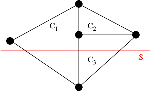
In Figure 1(a) a two-dimensional slice of three, three-dimensional cones is shown. The cones and are both adjacent to along the same facet. However the affine subspace does not intersect and therefore is not adjacent to .
In Figure 1(b) we consider the complementary basis and the cone . The goal is to find the critical domain that is adjacent to . The inequality is not redundant in and therefore the hyperplane defines a facet of . Since is equal to , we have that is adjacent to . The other inequality is redundant in and therefore the critical domain is not adjacent to .
5 Extension of the algorithm for not in general position
The previous section presented an algorithm that enumerates all feasible bases and returns the graph of critical domains. The algorithm works only under the assumption that the image of the parametrisation lies in general position; Assumption 4.2. However, this assumption is not realistic and it is highly desirable to remove it.
In the case of degeneracy (i.e. is not in general position), Propositions 3.21 and 3.25 are no longer valid, as can be seen in Example 2. Therefore, during neighborhood computation it is not sufficient to explore only the adjacent complementary cones. In order to extend the algorithm to the degenerate case, we apply a symbolic perturbation technique (the lexicographic perturbation) which has the effect of shifting into general position.
The next subsection will demonstrate how to handle the perturbation for neighborhood computation, in particular lines 5 and 11 of Algorithm 2. By using this technique we obtain a graph of critical domains relative to the perturbed affine subspace , which can differ from the graph of critical domains relative to . In particular, some full-dimensional critical domains in may be non full-dimensional in . We will see that there exists a subgraph of that is a graph of critical domains relative to and which can be obtained by postprocessing .
Example 2.
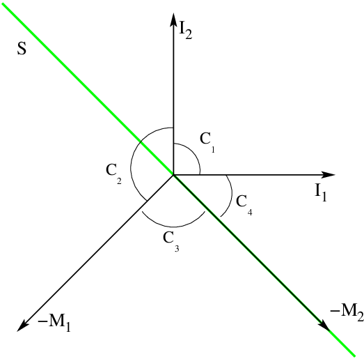
This example demonstrates the effect when a parametric LCP is not in general position. Consider the parametric LCP defined by the matrices
A figure depicting the complementary cones relative to and of the affine subspace is shown in Figure 2. Let , , and . For notational simplicity, we denote by the complementary cones and by for the critical domains. Clearly does not lie in general position because it intersects and on their boundary but not in their interiors. Proposition 3.21 is violated because is neither empty nor full-dimensional, and furthermore and are equal and hence . Theorem 3.25 is violated because and are adjacent, but and are not.
5.1 Lexicographic perturbation
This section presents a well-known method that permits the perturbation of the image of the parametrisation into general position and which can be treated symbolically: the lexicographic perturbation.
We introduce the following notation that will be used for the reminder of the paper.
Definition 5.1.
The vector is called the lexicographic perturbation vector and is a function of a positive real number .
We denote with the affine subspace perturbed by
| (5.20) |
Theorem 5.2.
Let be a sufficient matrix and be the affine subspace for a given matrix and a vector . There exists a such that lies in general position for each .
Remark 5.3.
In the remainder of the paper we will use the standard expression “property A holds for all sufficiently small ” rather than the more cumbersome “there exists such that property A holds for each ”. Therefore the claim of Theorem 5.2 can be written as: lies in general position for all sufficiently small .
To prove Theorem 5.2, we need the following lemma.
Lemma 5.4.
Let , and . For any complementary cone , there exist finitely many such that intersects but not .
Proof.
Let be a complementary basis. We denote with the hyperplane for all . Therefore is a facet of . We will prove that for any subset there are finitely many such that the following condition holds
| (5.21) |
The statement of the lemma will then follow directly, since there are finitely many subsets of .
Let be any nonempty subset of . For any for which (5.21) holds, contains the indices of all inequalities of that are implicit equalities and it holds that
| (5.22) |
where .
We can distinguish two cases. The case 1: there exists such that is a zero row vector. Since is nonempty, for the condition (5.22) to be valid. This non-trivial polynomial equation holds for at most values of .
Now consider the case 2: has no zero rows. We will prove that the matrix does not have full row rank. Since is nonempty and has dimension , the Chebyshev center problem has an optimal value of zero, i.e. . We consider its dual problem
| (5.23) |
From strong duality, there exists a non-zero optimal solution such that and . We now claim that all indices of the strictly positive components of are contained in . Assume that there is an index with . Then, for any , , i.e. , which contradicts the maximality condition in (5.21). Therefore, and , i.e. there exists a non-trivial combination of rows of .
Let be a set of columns of such that , , form a basis of the column space of . Since does not have full row rank, . If are linearly independent then for any the equation (5.22) cannot hold. We claim these vectors are linearly dependent for finitely many .
First we consider the case . Then, these vectors are linearly dependent if and only if
| (5.24) |
This condition is a polynomial equation in and holds for finitely many . Finally, if
, we use the same
argument by adding a proper number of vectors such that
are linearly independent vectors.
∎
Proof of Theorem 5.2.
We can assume without loss of generality that does not lie in general position. For any complementary cone exactly one of the following cases holds:
- 1.
does not intersect ,
- 2.
intersects the interior of ,
- 3.
intersects the boundary of and , which can be differentiated into two subcases:
- (a)
such that for all
- (b)
For all there exists an such that .
- (a)
For each of these cases we need to prove that there exists such that either intersects for all or for all . Clearly, this condition holds for cases 1, 2 and 3a. Therefore, it suffices to prove that for case 3b there exists a such that intersects for all .
Let be any complementary cone that satisfies condition 3b. From Lemma 5.4 and by assumption there exists a such that intersects the interior of and for any either or . More precisely, one can select any smaller than the smallest for which intersects but not . Since shifts continuously with , there exists no such that . ∎
Example 3.
Figure 3 shows two examples in which does not lie in general position. In the first example (Figure 3(a)) the cones and contain adjacent critical domains, although they are not adjacent cones. In the second example (Figure 3(b)) two different critical domains coincide. In higher dimensions the critical domains can overlap in several ways and therefore it is not evident how to choose an appropriate decomposition when this situation occurs. In both cases the affine subspace can be artificially and symbolically shifted into general position through the use of lexicographic perturbation.


5.2 Neighborhood computation in
Input:
A complementary basis , a sufficient matrix and an affine subspace .
Output:
The set of complementary bases , whose critical domains are adjacent to .
Given a complementary basis that is feasible in , the goal is to determine the adjacent critical domains to . Since lies in general position, it suffices to explore the adjacent bases of the basis . Similarly to the non degenerate case, we first determine the facets of at Line 5 of Algorithm 3 and then compute the adjacent critical domains that intersect with each facet.
Let be a complementary basis and consider , where . The hyperplane , for some intersected with forms a facet of if there exists a such that for all and . Therefore is a facet of if and only if
| (5.25) |
has a positive optimal value for all sufficiently small.
This decision problem is no longer an LP, because the right hand side of the constraints depends on a polynomial in and we want to know the behavior of in the neighborhood of zero. In the next subsection we will propose an efficient method for determining if is positive for sufficiently small .
If the hyperplane defines a facet of , then we can distinguish the same three cases as discussed in Section 4.1.
Diagonal pivot.
If there is exactly one adjacent complementary basis , then is full-dimensional (by the general position of ) and is the unique adjacent critical domain to along .
Boundary of .
If there are no adjacent complementary cones to along (see Corollary 3.15), then there is no adjacent critical domain to along the facet
Exchange pivot.
If there are adjacent bases with and , then we must check for each such basis whether (Line 11 of Algorithm 3). Assume where . As in the non-degenerate case, we formulate a decision problem similar to LP (4.19) to test the dimension of the intersection:
| (5.26) |
where and . The two critical domains are adjacent, i.e. , in for all sufficiently small if and only if for all sufficiently small .
5.2.1 Symbolic computation of the parametric Chebyshev center problem
As seen in the previous subsection, the goal is to decide whether the optimal value of (5.25) (and of (5.26)) is positive for all sufficiently small . We call this decision problem a parametric Chebyshev center problem. Here we introduce a method that can compute exactly the behavior of for sufficiently small positive ; the proposed approach is summarized as Algorithm 4. The procedure is explained only for (5.25), since the same method can be easily applied for (5.26). The goal is to transform (5.25) into a multi-objective LP that can then be solved with any LP-solver. Recall the parametric LP (5.25):
| (5.27) |
For a fixed value of , this is a linear program and its dual is:
| (5.28) |
Let us denote its feasible region by , that is,
| (5.29) |
In order to solve (5.28) symbolically we introduce the following standard notion.
Definition 5.5 (Lexico-positive).
A vector is lexico-positive (denoted by ), if and the first non-zero component of is strictly positive. Given two vectors and , we write if and only if . A matrix is called lexico-positive if all its rows are lexico-positive. If is a set of vectors, then is the lexico minimum of S if and only if for each .
The following theorem demonstrates that minimizing the polynomial cost function of (5.28) is equivalent to computing the lexicographic minimum of a vector.
Theorem 5.6.
If is a feasible vector of the dual problem (5.28), then the two statements below are equivalent:
- 1.
such that for all ,
- 2.
.
Proof.
The statement follows from the equality , which holds for all and for all . For every polynomial the following holds: there exists a such that for all if and only if the first non-zero coefficient of is positive, i.e. is lexico positive. ∎
We can now consider an equivalent problem that we call a lexicographic linear program (lexLP):
| (5.30) |
The cost of this optimization problem is vector valued and the operator means to compute the lexicographic minimum vector over all feasible decision variables . We will denote this particular lexLP, which tests the redundancy of the -th inequality in , as the function .
Theorem 5.7.
Proof.
The statement is a direct consequence of Theorem 5.6. ∎
Note that as is the case for linear programs, the restrictions and the objective function of (5.30) are linear, although the objective returns a vector instead of a scalar. We say that is the optimal value of (5.30). If the vector is non-zero then the feasibility region is bounded and therefore the optimal value is always attained if the problem is feasible.
For our purposes, it is not necessary to compute the entire vector , but only a sufficient number of its elements in order to determine if it is lexico-positive or not. To this end, the goal is to find the first non-zero component of and therefore the lex min problem (5.30) can be treated as a multi-objective LP in the following way. First (say at step ) we solve the LP:
| (5.32) |
where . If then we can conclude that the optimal value of the problem (5.30) is lexico-positive or lexico-negative from the sign of . Otherwise, if does equal zero, then we must consider the next objective function and minimise it while maintaining , and so on.
If , then at the step we solve:
| (5.33) |
where and for . If is the first non-zero value of then of (5.30) is lexico-positive if and lexico-negative otherwise. The resulting procedure is Algorithm 4, where the feasible region of the LP (5.33) is denoted by .
Input:
Output:
Remark 5.8.
Note that the lexLP always has a non-zero optimal value because zero is not feasible in (5.33) and the optimal solution of the last LP (5.33), with , must be optimal also for all previous LPs. Since has full rank we must have that is non-zero and therefore there must be at least one component of that is non-zero.
The parametric LP (5.26) that determines whether two critical domains are adjacent can also be solved using the same procedure. LP (5.26) can be rewritten as a lex min LP as follows:
| (5.34) |
We will call this lexLP because it tests the adjacency of and . Recall that one of the two equalities in (5.26) can be removed because one is redundant and therefore one of and is also redundant. Hence, (5.34) has the same structure as (5.30) and can be solved as a multi-objective LP as explained above (see Algorithm 4).
5.3 Post-processing of the graph of critical domains
The previous section introduced a computational method for computing the graph of critical domains relative to the lex-perturbed space for all sufficiently small. The goal in this section is to recover the graph of critical domains relative to the original space according to Definition 3.23.
The following theorems will show that one can construct from the graph of critical domains relative to the unperturbed space .
Theorem 5.9.
Let be a sufficient matrix, an affine subspace and consider the graph of critical domains relative to the lexicographically perturbed space for sufficiently small . Let be the set of all bases in with full-dimensional critical domains . Then the following statements hold.
- 1.
For each , the complementary cone intersects and therefore is nonempty.
- 2.
For any two distinct bases and in , and have disjoint relative interiors.
- 3.
The set of all full-dimensional critical domains for covers , i.e.,
and forms a polyhedral decomposition of .
Proof.
First, note that complementary cones are closed and so the first statement follows directly.
To prove the second, note that for all sufficiently small (say ) lies in general position. From Proposition 3.25 the critical domains defined by are disjoint in their interiors for any positive . The second statement follows from the fact that for any basis , changes continuously in , for .
The third statement is proven in two steps. First we prove that the critical domains whose bases are in define a covering of . Let , since and is a convex cone, there exists a basis such that for all sufficiently small. Therefore is in and hence in because complementary cones are closed and thus . Since critical domains are closed and is a convex polyhedron, the full-dimensional critical domains define a covering of . ∎
The above theorem demonstrates that the bases in have nonempty critical domains in the unperturbed space . Moreover, there exists a subset whose critical domains form a polyhedral decomposition of according to Definition 3.23. The next theorem discusses how adjacency in relates to adjacency in .
Theorem 5.10.
Let be a sufficient matrix and be two complementary bases in , i.e. and both have dimension . If and are adjacent, then there exists a path in from to with the following property: intersects with dimension , i.e. for all .
Proof.
If and are adjacent, is clearly the desidered path. We assume they are not adjacent. We choose a which is not contained in any critical domain or in any face of dimension or less, and let be the parameter with . We look now (for a moment) at the parameter space and at the critical regions. The hyperplane contains the intersecion of the two critical regions, i.e. and consider its perpendicular (normal?) line . The image of is in the original space , respectively in the perturbed space .
We know that for each sufficiently small every critical domain becomes either full-dimensional or empty. The full-dimensional ones vary continuously in function with . Consider a segment of the line such that it intersects either and for all sufficiently small. Because of the continuity no critical domain, which has dimension smaller than in the original space intersects this segment for all sufficiently small. Similarly, for any no face of of dimension smaller than intersects for all sufficiently small. The desidered path is given by the critical domains which decompose the line segment between and . ∎
Note that the last condition in the above theorem, along with Proposition 3.21, implies that for and therefore Theorems 5.9 and 5.10 imply the following corollary.
Corollary 5.11.
Let be a sufficient matrix, an affine subspace and let be the graph of critical domains relative to . Then, the graph of critical domains relative to is related to as follows:
- 1.
- 2.
For every basis , has dimension .
- 3.
For each pair of bases and , the critical domains and are adjacent if and only if there exists a path in with , and for (or ).
The above corollary provides a simple procedure for computing a critical region graph relative to the unperturbed affine set from the perturbed one . We begin from the perturbed critical region graph and remove each node from that has a critical domain which is not full-dimensional and add all new edges to satisfying the statement 3 of Corollary 5.11. From Theorem 5.9, the critical domains of the nodes of the resulting graph will form the desired polyhedral covering of the . Theorem 5.10 states that the resulting graph contains edges for all adjacent bases, but may be overconnected since some of the critical domains of removed bases may have had a dimension less than . It remains, therefore, to test each edge in order to determine if the connected bases are in fact adjacent in the unperturbed space. As discussed previously, both operations for testing full-dimensionality and adjacency can be posed as linear programs.
Remark 5.12.
Note that much of the computation required to test for full-dimensionality of the critical domains for the unperturbed affine set has already been done while building the perturbed graph. Specifically, one can determine if a region is full-dimensional by examining the first component of the optimizer of LP (5.30).
6 Complexity of the algorithm
In this section we will discuss the complexity of the proposed algorithm, which enumerates all full-dimensional critical domains relative to the lexicographically perturbed affine subspace . The well-known example by Murty (see [21] or see Chapter 6 in [22]), which was used to prove the non-polynomiality of the Lemke and the principal pivoting methods, can be easily seen to demonstrate that the number of critical domains of a pLCP with an affine subspace of dimension and -matrix is exponential in . Since the complexity of the graph search (Algorithm 1) is a polynomial function of the number of critical domains, no algorithm for pLCP is polynomial in . It is, however, possible to bound the number of operations required to explore the neighborhood of each critical domain, i.e. the complexity of Algorithms 2 and 3. Since each critical domain will be explored exactly once, we can say that the algorithm is output sensitive in that its complexity is a polynomial function of the number of full-dimensional critical domains and the size of input, provided that a polynomial-time algorithm for linear programming is used.
We first consider the general position case and study the complexity of Algorithm 2. Assume that is of order , the affine subspace is of dimension and let be a complementary basis with a nonempty critical domain . The main computations of the function (Algorithm 2) are:
- •
- •
We denote the time necessary to solve an LP in standard form by , where var denotes the number of (nonnegative) variables and eq is the number of equality constraints. The time necessary to explore a critical domain can then be bounded as follows.
Theorem 6.1.
Let be a sufficient matrix and assume that the affine subspace lies in general position. For each complementary basis with a nonempty critical domain the time necessary to explore the neighborhood of is bounded by:
| (6.35) |
Proof.
Redundancy checking requires the solution of LP (5.28) once for each of the inequalities of , which takes time. Adjacency checking by solving the LP (4.19) is necessary only in the case that the considered adjacent basis differs by two elements from the basis and since there are at most such bases, the second term follows. ∎
If does not lie in general position, then the lexLPs (5.30) and (5.34) are solved instead of LPs (4.18) and (4.19). Each lexLP can be solved as a sequence of at most LPs with the same variables and constraints (see Algorithm 4), which leads to the following complexity bound.
Theorem 6.2.
If is a sufficient matrix, then for each complementary basis with nonempty critical domain the time necessary to explore the neighborhood of can be bounded by
| (6.36) |
The above theorems bound the complexity of “exploring” a basis of the output in Algorithm 1 (Line 5). The condition at Line 6, which can be verified in time bounded by the logarithm of the size of the output, ensures that each output basis is explored exactly once. As a result, the complexity of the algorithm grows linearly with the size of the output and so is output sensitive.
7 Example
In this section we present a simple illustrative example that arises from control theory. Consider the following discrete time constrained linear time-invariant system:
where is the system state, is the successor state and is the system input. A common method of control for this class of systems is Model Predictive Control, in which we solve at each point in time the following finite horizon optimal control problem:
| subject to | ||||
| (7.37) |
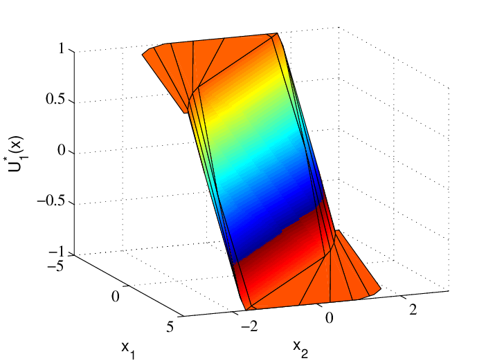
where is the current state of the system, the prediction horizon is and the weighting matrices , and are the identity. For high-speed systems, such as electric power converters, the goal is to solve the above quadratic program as rapidly as possible, in some cases at rates exceeding hundreds of kilohertz (e.g. [3]). By computing the optimizer offline as an explicit piecewise-affine function of the state , these speeds can be achieved [25, 14, 4]. The above parametric quadratic program is easily converted to a pLCP with a positive semi-definite matrix [22], which was then solved using the proposed algorithm. The resulting polyhedral partition and mapping from the parameter to the optimizer is shown in Figure 4.

8 Conclusion
In this paper an algorithm to enumerate all feasible bases of the parametric LCP defined by a sufficient matrix and a lexicographically perturbed affine subspace was proposed. It has been shown that the perturbed parametric LCP can be solved in a time linearly bounded by the size of the output and moreover, this output can be efficiently post-processed in order to generate a polyhedral decomposition for the unperturbed original affine subspace .
One feature of the algorithm which is not ideal is the space requirement. Namely, the proposed algorithm must store all discovered feasible bases in the memory because it relies on the standard graph search technique. A great improvement can be made if we could apply the reverse search technique [1] which is essentially memory free. For this, it is necessary for the underlying graph to be oriented properly with exactly one sink. Somewhat similar to the present work, the paper [9] proposed an algorithm to compute a polyhedral complex known as the Gröbner fan which was shown to have such a “reverse search property.” Finding such an orientation for the graph of critical domains is an excellent subject of the future research.
References
- [1] D. Avis and K. Fukuda. Reverse search for enumeration. Discrete Applied Mathematics, 65:21–46, 1996.
- [2] G. Bank, J. Guddat, D. Klatte, B. Kummer, and D. Tammer. Non-linear Parametric Optimization. Akademie-Verlag Berlin, 1983.
- [3] A.G. Beccuti, G. Papafotiou, R. Frasca, and M. Morari. Explicit Hybrid Model Predictive Control of the dc-dc Boost Converter. In IEEE PESC, Orlando, Florida, USA, June 2007.
- [4] A. Bemporad, M. Morari, V. Dua, and E. N. Pistikopoulos. The explicit linear quadratic regulator for constrained systems. Automatica, 38(1):3–20, January 2002.
- [5] F. Blanchini. Set invariance in control - a survey. Automatica, 35(11):1747–1768, November 1999.
- [6] R.W. Cottle, J.-S. Pang, and R.E. Stone. The Linear Complementarity Problem. Academic Press, 1992.
- [7] R.A. Danao. On the parametric linear complementarity problem. Journal of Optimization Theory and Applications, 95(2):445–454, November 1997.
- [8] B. De Schutter and B. De Moor. The extended linear complementarity problem. Mathematical Programming, 71(3):289–325, December 1995.
- [9] K. Fukuda, A. Jensen, and R. Thomas. Computing Gröbner fans. Mathematics of Computation, 76:2189–2212, 2007.
- [10] K. Fukuda, M. Namiki, and A. Tamura. EP theorems and linear complementarity problems. Discrete Applied Mathematics, 84:107–119, 1998.
- [11] K. Fukuda and T. Terlaky. Linear complementarity and oriented matroids. Journal of the Operations Research Society of Japan, 35:45–61, 1992.
- [12] J.E. Goodman and J. O’Rourke, editors. Handbook of discrete and computational geometry. CRC Press, Inc., Boca Raton, FL, USA, 1997.
- [13] J. Hooker. Logical inference and polyhedral projection. pages 184–200. 1992.
- [14] T. A. Johansen, I. Petersen, and O. Slupphaug. On explicit suboptimal LQR with state and input constraints. In Decision and Control, 2000. Proceedings of the 39th IEEE Conference on, volume 1, pages 662–667 vol.1, 2000.
- [15] C. N. Jones, E. C. Kerrigan, and J. M. Maciejowski. On polyhedral projection and parametric programming. Journal of Optimization Theory and Applications, 137(3), June 2008.
- [16] C.N. Jones, J.M. Maciejowski, and E.C. Kerrigan. Lexicographic perturbation for multiparametric linear programming with applications to control. Automatica, 43(10):1808–1816, October 2007.
- [17] C.N. Jones and M. Morari. Multiparametric Linear Complementarity Problems. In IEEE Conference on Decision and Control, December 2006.
- [18] L.P. Kaelbling, M.L. Littman, and A.R. Cassandra. Planning and acting in partially observable stochastic domains. Artificial Intelligence, 101:99–134, 1998.
- [19] D. Klatte. On the Lipschitz behavior of optimal solutions in parametric problems of quadratic optimization and linear complementarity. Optimization, 16:819–831, 1985.
- [20] M. Kojima, N. Meggiddo, T. Noma, and A. Yoshise. A unified approach to interior point algorithms for linear complementarity problems, volume 538 of Lecture Notes in Computer Science. Springer-Verlag, 1991.
- [21] K. G. Murty. Computational complexity of complementary pivot methods. Mathematical Programming Study 7, pages 61–73, 1978.
- [22] K. G. Murty and F. T. Yu. Linear Complementarity, Linear and Nonlinear Programming. Helderman-Verlag, 1988.
- [23] J. Ponce, S. Sullivan, A. Sudsang, J. Boissonnat, and J. Merlet. On computing four-finger equilibrium and force-closure grasps of polyhedral objects. International Journal of Robotics Research, February 1995.
- [24] S. Sankaranarayanan, F. Ivančić, and A. Gupta. Program analysis using symbolic ranges. pages 366–383. 2007.
- [25] M. M. Seron, G. C. Goodwin, and J. A. De Doná. Geometry of model predictive control for constrained linear systems. Technical Report EE0031, The University of Newcastle, Australia, 2000.
- [26] K. Tammer. Parametric linear complementarity problems. [Online: Stand 2008-04-29T15:56:22Z].
Appendix A Useful properties of matrix classes
This section gives an overview of some matrix classes with important properties for linear complementarity
problems. The reader is referred to [6] for a thorough survey.
-Matrices
Definition A.1.
The matrix is a -matrix if and only if all principal minors of are strictly positive.
This class characterizes the matrices for which the corresponding LCP always has a unique solution.
Theorem A.2.
The following statements are equivalent:
- 1.
,
- 2.
The LCP defined by the matrix has a unique solution for all right hand side vectors ,
- 3.
does not reverse the sign of any nonzero vectors, i.e.
Recall that is a positive definite matrix, denoted with if for all it holds that . It is then easy to see from the above theorem that positive definite matrices belong to the class .
-matrices
Definition A.3.
The matrix is a -matrix if and only if all principal minors of are non-negative.
Analogously to the positive-definite case above, positive-semidefinite matrices (PSD) are clearly in . The following theorem gives properties of PSD matrices relevant to the solution of pLCPs.
Theorem A.4.
Let be a matrix and be the identity matrix of the same order. The following statements are equivalent:
- 1.
,
- 2.
For each vector there exists an index such that and ,
- 3.
is a matrix for all .
Semimonotone matrices
Definition A.5.
A matrix is called semimonotone if the following holds:
| (1.38) |
The class of such matrices is denoted by and by Theorem A.4, every -matrix is semimonotone.
Definition A.6.
Let be a semimonotone matrix. If for all index subsets with the principal pivot transform of with respect to
is semimonotone, then is called fully semimonotone. The class of such matrices is denoted with and is said to be an -matrix.
-Matrices
Definition A.7.
An LCP defined by the matrix and right hand side vector is called weakly feasible if there exist positive vectors and such that and feasible if also holds. The class of matrices for which the LCP is feasible whenever it is weakly feasible, is denoted by .
Since -matrices are feasible for each vector , they are also -matrices.
Theorem A.8.
Let and be the identity matrix of same order. The following statements are equivalent:
- 1.
,
- 2.
The complementary range is convex,
- 3.
The implications of convexity of the complementary range are discussed in the next section.
Sufficient Matrices
Definition A.9.
A square matrix is called column sufficient if it satisfies the implication:
| (1.39) |
The matrix is called row sufficient if its transpose is column sufficient. If is both column and row sufficient, then it is said to be sufficient.
Theorem A.10.
If is row sufficient matrix, then
- 1.
,
- 2.
.
From the theorem above we have that every column sufficient matrix also belongs to . Below we state a characterisation of column sufficient matrices, which has an important implication regarding the structure of the resulting complementary cones.
Theorem A.11.
Given a matrix , the following statements are equivalent:
- 1.
is column sufficient,
- 2.
For each vector the following holds: if are two solutions of the LCP defined by the matrix and the vector , then .