The Effect of the Sparticle Mass Spectrum on the

In many leptogenesis and baryogenesis scenarios [1, 2, 3, 4, 6, 5, 7, 8], conserved charges associated with baryon minus the lepton number ($B-L$ or $B/3-L_{i}$) are generated by out-of-equilibrium dynamics. Subsequently, $B-L$ or $B/3-L_{i}$ is converted to the observed baryon number $B$ by non-perturbative ${\rm SU}(2)_{L}$ operators, which are in equilibrium until the time of the electroweak phase transition. Many papers [9, 10, 11, 12, 13, 14, 15, 16] have thus investigated the relationship between $B-L$ or $B/3-L_{i}$ and $B$. To leading order in perturbative expansion, the relationship between $B-L$ and $B$ that is used in the literature is that of Ref. [11]. For example, in MSSM-like situations with two Higgs doublets, assuming a strong first order phase transition, the formula

is often used to convert the $B-L$ generated by thermal leptogenesis into the observed baryon asymmetry [4]. In this article, we point out that kinematics associated with beyond the Standard Model (SM) particles can significantly change this kind of formula such that the usage of Eq. (1) is incorrect. Although “typical” changes in the formula are modest, in some cases the change may be an order of magnitude or may even lead to a sign flip between $B$ and $B-L$, even within just the Minimal Supersymmetric Standard Model (MSSM) particle content. In the case that the constant of proportionality between $B$ and $B-L$ is increased from the standard value, the well known reheating temperature bounds associated with gravitinos [17, 18, 19] may be mildly relaxed.

Although the effects of particle content and kinematics on the relationship between $B$ and $B-L$ have been discussed to some extent before [13, 12], we contribute the following, using the MSSM spectrum to make the illustration concrete:

1. 1.

   We give a closed form expression relating $B$ to $(B-L)$ or $(B/3-L_{i})$ that includes all the sparticle kinematic effects.

2. 2.

   We point out that there are situations where $B$ and $B-L$ can have opposite signs, or $B$ can be larger than some of the typical values used in the literature.

3. 3.

   Even when some sparticles are heavier than the temperature, equilibrium can be maintained, although its effect on the system will become smaller as the number density becomes Boltzmann suppressed.

4. 4.

   Even if gauginos are extremely heavy, “superequilibrium” — namely, chemical equilibrium between a particle and its superpartner — is maintained through Yukawa interactions.

Although the latter two points have been discussed in the context of electroweak baryogenesis in [20], they are also important for lepto-/baryogenesis scenarios involving the conversion from $B-L$ to $B$.

The order of presentation will be as follows. In the next section we briefly discuss the intuition for the $B-L$ to $B$ conversion. In Sec. 3, the formulae relating $B-L$ (or $B/3-L_{i}$) to $B$ are derived. Sec. 4 discusses the range of possible numerical effects coming from the derived formulae. We then conclude with a brief summary.

We briefly sketch the main physical point of this work such that the reader may gain some intuition. Suppose, at some early time, with temperature $T\gg 100$ GeV, $(B-L)$ is generated. Although $(B-L)$ is approximately conserved, individually $B$ and $L$ are affected by the non-perturbative ${\rm SU}(2)_{L}$ operator; this process is in equilibrium and leads to the condition that

where the subscript _L refers to baryon and lepton number in left handed fermions. (In Eq. (2), we have assumed that the thermal masses of quarks and leptons are light compared to the temperature. Recall we are considering a situation before the electroweak phase transition, when SM fermions have no Higgs-vev-induced masses.) It is important to note that Eq. (2) is valid even though for each sphaleron transition $\Delta B_{L}=-\Delta L_{L}$. The different numerical coefficient arises because there is a factor counting the degrees of freedom in the Boltzmann equations which ultimately leads to the equilibrium condition of Eq. (2). If $(B-L)$ was generated solely for left handed fermions, and if it remained solely with left handed fermions, we would have by Eq. (2)

which incidentally differs from the introductory estimates of [11]because there, $B_{L}+L_{L}=0$ is assumed instead of Eq. (2). However, there exist additional interactions in equilibrium — Yukawa and (possibly) gaugino interactions — which flip chirality and convert quarks and leptons into squarks and sleptons. Therefore, we need to keep track of the baryon/lepton content in scalars and right handed fermions, denoted by _S and _R, respectively. The total baryon and lepton numbers are

Using Eqs. (2, 4), we have

Therefore, we see that the deviation of $B$ from $(B-L)/4$ depends on how much lepton and baryon density is present in scalars and right handed fermions. These scalar and right handed densities depend sensitively on their masses. For example, if squark and sleptons are heavy, then their equilibrium densities will be small; the impact of $B_{S}$ and $L_{S}$ in Eq. (5) will be small. However, if they are light (compared to the temperature at which non-perturbative ${\rm SU}(2)_{L}$ processes fall out of equilibrium), their equilibrium densities – and their impact in Eq. (5) – may be significant.

In this section, we derive explicit expressions relating $B$ to (a) $B-L$ in the situation in which the lepton chemical potentials of different flavors are in equilibrium, or (b) $B/3-L_{i}$ in the situation in which they are not in equilibrium.

Consider the physical situation after the freeze out of $B-L$ or $B/3-L_{i}$ and before the electroweak phase transition at $T=T_{c}$. As always, Boltzmann equations govern the chemical potentials of all the particle species. The reaction rates for the Boltzmann equations are temperature dependent and the chemical potentials will adjust themselves depending on the strength of interactions rates. What is important for the baryon asymmetry is the time period close to the electroweak phase transition, the completion of which will effectively shut off the $B+L$ violating reactions. Close to this time period at $T\approx 100$ GeV, the Hubble expansion rate is $H\sim 10^{-14}$ GeV. Hence, even a very small interaction (e.g. those suppressed by small Yukawa couplings) can be in equilibrium.

We denote the chemical potential of a particle $X$ by $\mu_{X}$. Under the assumption of kinetic equilibrium and for small $\mu_{X}/T$, the relation

between the charge density and the chemical potential holds, where

The $+$ sign holds here for fermions and $-$ for bosons. In the massless limit, $k_{X}(0)$ evaluates to $1$ for fermions and $2$ for bosons. This is useful for determining the equilibrium value of the baryon density $B$. In order to compare with Ref. [11], but also for an easier evaluation of the final result, we do not absorb the factor $g_{X}$ taking account of the internal colour and isospin degrees of freedom in our definition of $k_{X}$.

In order to calculate $B$, one makes use of the fact that certain reactions are in chemical equilibrium and that there are conserved charges. We collectively denote the arising conditions as equilibrium assumptions. For the MSSM, they can be stated as follows:

1. (a)

   Isospin violating interactions mediated by $W^{\pm}$ bosons are in equilibrium. This implies that

   	$\displaystyle\mu_{Q^{i}}\!\!\!$	$\displaystyle=$	$\displaystyle\!\!\!\mu_{u^{i}_{L}}=\mu_{d^{i}_{L}}\,,\quad\mu_{\widetilde{Q}^{i}}=\mu_{\widetilde{u}^{i}_{L}}=\mu_{\widetilde{d}^{i}_{L}}\,,$		(8)
   	$\displaystyle\mu_{L^{i}}\!\!\!$	$\displaystyle=$	$\displaystyle\!\!\!\mu_{\nu^{i}_{L}}=\mu_{e^{i}_{L}}\,,\quad\mu_{\widetilde{L}^{i}}=\mu_{\widetilde{\nu}^{i}_{L}}=\mu_{\widetilde{e}^{i}_{L}}\,,$
   	$\displaystyle\mu_{H}\!\!\!$	$\displaystyle=$	$\displaystyle\!\!\!\mu_{H_{1}^{+}}=\mu_{H_{1}^{0}}=\mu_{H_{2}^{+}}=\mu_{H_{2}^{0}}\,.$

   For the last equality, we have also assumed equilibrium of Yukawa interactions, as listed below. Note that due to the mass-degeneracy of particles in an isospin doublet, isospin equilibrium here also implies the absence of the charge density $T^{3}$ of weak isospin .

2. (b)

   Yukawa interactions of Standard Model Particles are in equilibrium,

   $\displaystyle\mu_{Q^{i}}+\mu_{H}=\mu_{u^{i}}\,,\quad\mu_{Q^{i}}-\mu_{H}=\mu_{d^{i}}\,,\quad\mu_{L^{i}}-\mu_{H}=\mu_{e^{i}}\,.$

   (9)

   Note that these conditions are automatically consistent with the ${\rm SU}(3)_{C}$ non-perturbative chiral flip processes being in equilibrium,

   $$\sum\limits_{i=1}^{3}\left\{2\mu_{Q^{i}}-\mu_{u^{i}}-\mu_{d^{i}}\right\}=0\,.$$

   (10)

3. (c)

   Flavor changing interactions in the baryonic sector are in equilibrium. This allows us to write

   $\displaystyle\mu_{Q}\!\!\!$

   $\displaystyle=$

   $\displaystyle\!\!\!\mu_{Q^{1}}=\mu_{Q^{2}}=\mu_{Q^{3}}\,,\quad\mu_{u}=\mu_{u^{1}}=\mu_{u^{2}}=\mu_{u^{3}}\,,\quad\mu_{d}=\mu_{d^{1}}=\mu_{d^{2}}=\mu_{d^{3}}\,.$

   (11)

4. (d)

   As a initial condition, the Universe is neutral with respect to gauge charges. This means, all charges associated with commuting generators of local symmetries are imposed to vanish. We have already implicitly incorporated neutrality with respect to isospin $T^{3}$, associated with the diagonal generator of ${\rm SU}(2)_{L}$, as well as neutrality with respect to color charges. In addition, we also demand hypercharge-neutrality,

   $$Y=0\,.$$

   (12)

5. (e)

   The ${\rm SU}(2)_{L}$ non-perturbative process is in equilibrium, implying

   $$\sum\limits_{i=1}^{3}\left(3\mu_{Q^{i}}+\mu_{L^{i}}\right)=0\,.$$

   (13)

6. (f)

   There are primordial $B/3-L_{i}$ asymmetries, which possibly originate from GUT-baryogenesis or leptogenesis, but which are conserved at lower temperatures, such as the electroweak scale.

7. (g)

   Yukawa and triscalar interactions involving supersymmetric partners of SM particles are in equilibrium,

   	$\displaystyle\mu_{\widetilde{Q}^{i}}+\mu_{H}=\mu_{\widetilde{u}^{i}}\,,\quad\mu_{\widetilde{Q}^{i}}-\mu_{H}=\mu_{\widetilde{d}^{i}}\,,\quad\mu_{\widetilde{L}^{i}}-\mu_{H}=\mu_{\widetilde{e}^{i}}\,,$		(14)
   	$\displaystyle\mu_{\widetilde{Q}^{i}}+\mu_{\widetilde{H}}=\mu_{u^{i}}\,,\quad\mu_{\widetilde{Q}^{i}}-\mu_{\widetilde{H}}=\mu_{d^{i}}\,,\quad\mu_{\widetilde{L}^{i}}-\mu_{\widetilde{H}}=\mu_{e^{i}}\,,$
   	$\displaystyle\mu_{Q^{i}}+\mu_{\widetilde{H}}=\mu_{\widetilde{u}^{i}}\,,\quad\mu_{Q^{i}}-\mu_{\widetilde{H}}=\mu_{\widetilde{d}^{i}}\,,\quad\mu_{L^{i}}-\mu_{\widetilde{H}}=\mu_{\widetilde{e}^{i}}\,.$

8. (h)

   Chemical equilibrium between particles and their superpartners (“superequilibrium”) holds,

   	$\displaystyle\mu_{\widetilde{Q}^{i}}\!\!\!$	$\displaystyle=$	$\displaystyle\!\!\!\mu_{Q^{i}}\,,\quad\mu_{\widetilde{u}^{i}}=\mu_{u^{i}}\,\quad\mu_{\widetilde{d}^{i}}=\mu_{d^{i}}\,,$		(15)
   	$\displaystyle\mu_{\widetilde{L}^{i}}\!\!\!$	$\displaystyle=$	$\displaystyle\!\!\!\mu_{L^{i}}\,,\quad\mu_{\widetilde{e}^{i}}=\mu_{e^{i}}\,,$
   	$\displaystyle\mu_{\widetilde{H}}\!\!\!$	$\displaystyle=$	$\displaystyle\!\!\!\mu_{H}\,.$

   Obviously, these relations may be maintained through the absorption or emission of gauginos. In addition, as observed in Ref. [20], this assumption follows automatically, provided the conditions (b) and (g) hold.

As far as SM particles are concerned, it is well known that conditions (a–f) hold (see, e.g. [11, 12]). For example, to justify assumption (b), we consider the electron Yukawa coupling $h_{e}$, which is the smallest within the Standard Model sector. From the electron mass, we can infer that the electron Yukawa coupling $h_{e}$ fulfills $h_{e}\stackrel{{\scriptstyle>}}{{{}_{\sim}}}2.9\times 10^{-6}$, where equality would apply to the limiting case $\tan\beta=0$. We denote the thermally averaged net interaction rate for the process $e_{R}^{-}\leftrightarrow H^{0}+e_{L}^{-}$ as $\Gamma_{h_{e}}$, which is to be compared with the Hubble rate

For the purpose of our estimates, we take here and in the following the electroweak temperature to be $T=100\,{\rm GeV}$ and the effective number of degrees of freedom of the MSSM $g_{*}=228.75$. We remark that at the given temperature, the latter number depends on the sparticle masses, which is of no concern for the present estimates. If the thermally net averaged interaction rate for a Yukawa interaction of strength $h_{0}=1$ is given by $\Gamma_{h_{0}}$, then we find $\Gamma_{h_{0}}\stackrel{{\scriptstyle>}}{{{}_{\sim}}}0.03\,{\rm GeV}$ as a condition for the electron Yukawa rate $h^{2}_{e}\Gamma_{h_{0}}$ to be larger than $3H$. While the precise value of $\Gamma_{h_{0}}$ depends on the Higgs boson mass, we expect it at electroweak temperatures to be of order GeV (for $m_{H^{0}}=100\,{\rm GeV}$, $\Gamma_{h_{0}}=0.46\,{\rm GeV}$), such that electrons and left-handed neutrinos are in equilibrium.

For a generalization of the equilibrium conditions to the MSSM, we make use of the observation that in most of parameter space, condition (h) holds, such that we can the use a common chemical potential for particles and sparticles, $\mu_{X^{i}}=\mu_{\widetilde{X}^{i}}$ [20]. In order to express the charge densities then in terms of the common chemical potentials via relation (6), it is convenient to introduce the expressions

for all species except for the Higgs bosons and Higgsinos, for which we employ

We note that $k_{X}^{i}=2$ for a massless boson and $k_{X}^{i}=1$ for a massless fermion, while $k_{X}^{i}=0$ for both boson and fermion if their mass is much larger than $T$.

It has already been realized that if $T$ is much larger than the sparticle masses, the formula for converting $(B-L)$ to $B$ which is valid for a non-supersymmetric model also applies to the supersymmetric case, since the simple proportionality $\widetilde{X}^{i}=2X^{i}$ then holds for all species and one can use a common chemical potential [12]. In turn, the non-supersymmetric conversion formula is obviously also valid if $T$ is much smaller than the sparticle masses, simply because the sparticles physically decouple in that limit. In this paper, we make use of the fact that $\mu_{X^{i}}=\mu_{\widetilde{X}^{i}}$ is generically fulfilled in the MSSM at electroweak temperatures even in the intermediate regime, where sparticle masses are comparable to $T$. The resulting conversion formula is then found to depend on the sparticle masses.

A possible concern about the validity of assumption (h) may be that if the gaugino masses are way larger than $T$, particles and sparticles might not equilibrate. It turns out that this is not the case. If assumption (g) is valid, particle-sparticle equilibrium (15) follows algebraically when combining Eqns. (9) and (14) [20].

In order to argue why assumption (g) generically holds, we note that three-point interactions schematically contribute to the Boltzmann equations as

where $\Gamma$ denotes a thermally averaged net interaction rate as defined in [22]. We have extracted here a coupling constant $h^{2}$, which can be a Yukawa or a gauge coupling. An estimate for a certain three-body interaction to be in equilibrium then is¹¹ 1 More precisely, $X_{1}$ is in equilibrium if $h^{2}\Gamma_{h_{0}}^{(X_{1},X_{2},X_{3})}/{k_{1}}\stackrel{{\scriptstyle>}}{{{}_{\sim}}}3H$ and $X_{1,2}$ are in equilibrium. For the MSSM, the validity of assumption (g) can then be derived starting from the fact that Standard Model left- and right handed quarks and leptons are in equilibrium.

In Figure 1, we plot the thermally averaged net interaction rates for the Yukawa term $f_{1}{\widetilde{S}}{\widetilde{f}_{2}}$. All fields are taken here to be singlets, and factors of particle of multiplicity can easily be reinserted. The field $f_{1}$ is a light fermion, e.g. a quark, $\widetilde{S}$ another heavier fermion, e.g. the Higgsino, and $\widetilde{f}_{2}$ a scalar field, e.g. a squark, the mass of which we vary. When we increase the mass of $\widetilde{f}_{2}$, the equilibration rate $R$ is increasing, because the statistical factors $k_{i}$ grow faster than the thermally averaged net interaction rate $\Gamma$. Another feature that we see is that for $m_{\widetilde{f}_{2}}=m_{\widetilde{S}}$ the three-body process is kinematically forbidden, and the equilibration rate goes to zero. We expect that this kinematic blocking is circumvented through two by two processes involving the additional emission of a gauge boson from the quark or the squark.

Averaged triscalar rates are plotted in Figure 2. We consider the interaction $\mu\widetilde{f_{1}}S{\widetilde{f}_{2}}$, where all particles are now scalar and $\mu$ is a triscalar coupling which we take to be $\mu=100{\rm GeV}$. The fields $\widetilde{f}_{1,2}$ may be squarks and $S$ a Higgs boson. We see that even if we increase the individual masses beyond ${\rm TeV}$ scale, the equilibration rate remains to be of order ${\rm GeV}$, such that generically, the triscalar interactions are in equilibrium. Again, in certain kinematic regions, blocking occurs, which will be circumvented by gauge boson radiation.

We conclude that at electroweak temperatures, the equilibration rates $R$ are generically of order GeV, even for large sparticle masses. This means that Yukawa and triscalar interactions maintain chemical equilibrium, even if they are suppressed by couplings as small as $10^{-6}$. Since the light quark and lepton fields directly couple to the Higgs and sparticle fields through Yukawa interactions, the latter fields are therefore in chemical equilibrium, even if they are heavy. By the argument given in Ref. [20], this implies the chemical equilibrium of particles and sparticles, even if gauginos are very heavy.

We now explore the consequences of Eqs. (28) and (29), which are the main results of this paper. In particular, we give examples of the conversion factors for mass-spectrum scenarios which are usually considered in models of SUSY breaking as well as extreme cases, leading to maximal suppression or enhancement of the conversion factor. Note that as far as the summed factors of Eqs. (17) and (18) are concerned, the kinematic parameters must be in the range $3\leq\kappa_{X}\leq 9$ except for that of the Higgs, for which $2N_{h}\leq\kappa_{H}\leq 3N_{h}$ where $N_{h}$ is the number of Higgs doublets ($N_{h}=2$ for the MSSM which is the main illustrative model used in this paper). When all the sparticles are much heavier than the electroweak phase transition temperature and all the SM particles are light, $\kappa_{X\neq H}=3$ ($\kappa_{H}=2N_{h}$) while when all the sparticles are light, the other extreme value is taken. For $\kappa_{X^{i}}$ which has an unsummed family index, the values goes between $1$ (heavy sparticles and light SM particles) and $3$ (light sparticles and SM particles).

First, consider the lepton flavor equilibrium case of Eq. (28). We define the vector $\vec{\kappa}\equiv(\kappa_{Q},\kappa_{u},\kappa_{d},\kappa_{L},\kappa_{e},\kappa_{H})$ and give the following examples:

• •

  SM, which has no sparticles and only one Higgs doublet: $\vec{\kappa}=(3,3,3,3,3,2)$.

  $$B=\frac{28}{79}(B-L)\approx 0.35(B-L)$$

  (31)

• •

  Non-supersymmetric two Higgs doublet model: $\vec{\kappa}=(3,3,3,3,3,4)$.

  $$B=\frac{8}{23}(B-L)\approx 0.35(B-L)\,.$$

  (32)

  This is the value usually assumed in the literature for supersymmetric models, and its usage is sometimes erroneous.

• •

  Moderately light sleptons (e.g. $\tilde{m}_{L^{1},\;e^{1}}/T_{c}=1.6,\;\tilde{m}_{L^{2},\;e^{2}}/T_{c}=1.3,\;\tilde{m}_{L^{3},e^{3}}/T_{c}=1.1$) in MSSM (generic mSUGRA example): $\vec{\kappa}=(3,3,3,6,6,4)$.

  $$B=\frac{38}{167}(B-L)\approx 0.23(B-L)\,.$$

  (33)

  The baryon asymmetry in this generic scenario is therefore only $2/3$ of what is usually assumed.

• •

  The largest extreme value: $\vec{\kappa}=(9,3,9,3,3,4)$.

  $$B\approx 0.606(B-L)\,.$$

  (34)

  The baryon asymmetry is nearly 3 times that of Eq. (33). It turns out that the enhancement is most sensitive to $\kappa_{Q}$, i.e. it becomes large when left handed squarks are light.

• •

  The smallest extreme value: $\vec{\kappa}=(3,9,3,9,9,4)$.

  $$B\approx 0.079(B-L)\,.$$

  (35)

  Note that this $\vec{\kappa}$ corresponds to having light right handed up squarks, left handed sleptons, and right handed selectrons. It is also nearly “orthogonal” to the vector of the maximum value case, except for the $\kappa_{H}$ entry.

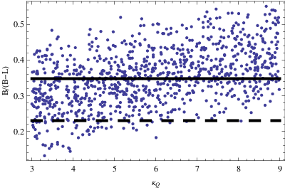
As a summary of the lepton flavor equilibrium case, see Fig. 3 to see the distribution of $B/(B-L)$ values. Since the purpose of this plot is to illustrate the range of kinematic possibilities, we do not analyze the phenomenological viability of every point in the scatter plot of Fig. 3 and make appropriate cuts.

Next, consider the lepton flavor violation case of Eq. (29). In this case, $B/(B-L)$ is sensitive to the magnitude and the signs of $B/3-L_{i}$ in addition to the $\kappa_{X}$. Hence, we have $B/(B-L)$ being a function of $\vec{P}$ defined as $\vec{P}\equiv(\kappa_{Q},\kappa_{u},\kappa_{d},\kappa_{L1},\kappa_{L2},\kappa_{L3},\kappa_{e1},\kappa_{e2},\kappa_{e3},\kappa_{H},B/3-L_{1},B/3-L_{2},B-L)$.

• •

  All sparticles heavy: $\vec{P}=(3,3,3,1,1,1,1,1,1,2N_{h},B/3-L_{1},B/3-L_{2},B-L)$.

  $$B=\frac{24+4N_{h}}{66+13N_{h}}(B-L)\,,$$

  (36)

  which is independent of individual $B/3-L_{i}$ and depends only on the sum $B-L$. It is also identical to Eqs. (31) and (32), and the result of [11].

• •

  Moderately light sleptons (e.g. $\tilde{m}_{L^{1},\;e^{1}}/T_{c}=1.6,\;\tilde{m}_{L^{2},\;e^{2}}/T_{c}=1.3,\;\tilde{m}_{L^{3},\;e^{3}}/T_{c}=1.1$) in MSSM (generic mSUGRA example): $\vec{P}=(3,3,3,1.85,2.01,2.13,1.85,2.01,2.13,4,B/3-L_{1},B/3-L_{2},B-L)$.

  $$B\approx 0.22(B-L)+0.03(B/3-L_{1})+0.01(B/3-L_{2})\,,$$

  (37)

  where care has been taken in preserving the precision such that the small corrections are not merely artifacts of the numerical truncation. It is clear that in this case, the result is very similar to Eq. (33) unless $(B/3-L_{1,2})$ is very different from $B-L$. In the limit that $L_{1}=L_{2}=L/3$, Eq. (33) is recovered.

• •

  Suppose $B/3-L_{3}=0$ such that $B/3-L_{2}=(B-L)-(B/3-L_{1})$. Then Eq. (37) becomes

  $$B\approx 0.23(B-L)+0.02(B/3-L_{1})\,.$$

  (38)

  If we let $r\equiv(B/3-L_{1})/(B-L)$, we have

  $$B\approx[0.23+0.02r](B-L)$$

  (39)

  Hence, even in the mSUGRA type of spectrum, the baryon number sign can flip relative to the $B-L$ sign, even if just two flavors contribute to the lepton asymmetry with opposite signs and fortuitously cancel with a fine tuning of about 0.1 (i.e. when $r\leq-12$).

  

• •

  A sign flip between $B-L$ and $B$ can be attained for example by the following mass spectrum which does not contain unrealistically many light sparticles and unrealistic cancellation of $B/3-L_{i}$: $\tilde{m}_{u^{n}}/T_{c}\approx 4-n$, and $\tilde{m}_{e^{1}}/T_{c}\approx 1$, $\tilde{m}_{L^{1}}/T_{c}\approx 1$ with $B/3-L_{1}=2(B-L)$, $B/3-L_{2}=-(B-L)$ and $B/3-L_{3}=0$ gives $\vec{P}=(9,9,3,3,1,3,3,1,1,4,2(B-L),-(B-L),B-L)$ and

  $$B\approx-0.05(B-L).$$

  (40)

  The dependence of this on one of the more sensitive mass parameters $\tilde{m}_{L}/T_{c}$ can be seen in Fig. 4.

• •

  A non-vanishing $B$ can be attained even with $B-L=0$. For example, if we choose $B/3-L_{1}=-(B/3-L_{2})$ and $B/3-L_{3}=0$, we have $B-L=0$ but $B\approx-0.08(B/3-L_{1})$ if we take $\tilde{m}_{e^{1}}/T_{c}\approx 1$.

To summarize the range of $B/(B-L)$ that can be attained for $B/3-L_{3}=0$, we make a scatter plot of $B/(B-L)$ as a function of $B/3-L_{1}$ in Fig, 5 marginalizing over the remaining free parameters of $\vec{P}$. Note that negative values of $B/(B-L)$ can be achieved without having a huge ratio of $(B/3-L_{1})/(B-L)$.

In gravity mediated SUSY breaking scenarios, an upper bound on the reheating temperature $T_{\textrm{RH}}$ exists due to gravitino decay effects on big bang nucleosynthesis which can be in conflict with a successful leptogenesis scenario [17, 18, 19]: i.e. $(B-L)_{\textrm{max}}=c_{1}T_{\textrm{RH}}<c_{1}T_{\textrm{max}}$ where $c_{1}$ is a constant and if we define $B=c_{2}(B-L)$ where $c_{2}$ is the constant that is the focus of this paper, we have $B_{\textrm{observed}}/|c_{2}c_{1}|<T_{\textrm{RH}}<T_{\textrm{max}}$. Hence, for those situations in which there is an enhancement of $c_{2}$, the squeeze on $T_{\textrm{RH}}$ can be relaxed. Although Fig. 5 looks naively as if a large enhancement can be achieved through the sparticle kinematic effects, because such large enhancement cases appear when there is a fine tuned cancellation between two $B/3-L_{i}$, such situations are unlikely to occur in realistic models. Milder enhancements (factor of 2 or 3) are however possible, and hence the lower bound on the reheating temperature can accordingly be reduced.

We have seen that the conversion factor may take a wide range of values, depending on the particular sparticle spectrum. Therefore, it is desirable to present a rule of thumb which applies at least to parametric scenarios that lead to a successful dark matter genesis and rely on minimal assumptions of parameters imposed at the Grand Unified scale. If we focus on the mSUGRA-inspired scenarios in Ref. [21], one of the simplifying assumptions for the Grand Unified scale is a common value for the squark and slepton masses $m_{0}$. The renormalization group running down to the ${\rm TeV}$ scale induces squark masses, that are typically large enough for $k_{\widetilde{Q}}^{i}=k_{\widetilde{u}}^{i}=k_{\widetilde{d}}^{i}=0$ to be a good approximation. The running of the slepton masses is less strong, such they may still be close to the electroweak scale. Among the sleptons, the running is typically more pronounced for the left handed particles, such that they are heavier than the right-handed ones. Finally, the bias due to the Yukawa couplings is less strong for leptons than for baryons, such that the case of approximate mass degeneracy for the different flavors is typical.

The size of the mass effects discussed within this paper for typical mSUGRA scenarios can be inferred from Table 1. We have taken the squarks to be infinitely massive and for the statistical factor of the Higgs-particles, we have set $\kappa_{H}=4$, corresponding to light Higgsinos and two light complex scalars, while the other two complex scalars are taken to be very heavy. We see that for light sleptons, $m_{\widetilde{L}}=150\,{\rm GeV}$ and $m_{\widetilde{e}}=100\,{\rm GeV}$, within this set of typical scenarios the baryon number is suppressed by roughly a factor of $2/3$, while for heavier sleptons, we approach the value $B/(B-L)\approx 0.35$, which is usually assumed. We note that none of these mSUGRA-motivated scenarios allows for a strong first order phase transition, such that in principle, effects of the onset of electroweak symmetry breaking need to be taken into account [14, 15], which we defer to future work.

Our analysis in this paper has assumed that the non-perturbative $B+L$ violating reactions involve only the chemical potentials of the left handed quarks and leptons. Ref. [23] has discussed the situation in which at high temperatures, the $\mu$-term and the gaugino mass terms may be neglected to enlarge the global symmetry group to include a combination of Peccei-Quinn and R-symmetry called $R_{2}$, such that the charge coupling anomalously to ${\rm SU}(2)_{L}$ is $B+L-R_{2}$, in which case the chemical potential constraints would change. However, since we are dealing with electroweak phase transition temperatures, $R_{2}$ is broken and the analysis returns to the usual non-perturbative $B+L$ violating reactions considered in this paper.

We have considered the kinematic effects on $B-L$ to $B$ conversion coming from the mass of the MSSM sparticles carrying $B$ and $L$. The contribution of scalars and right handed fermions carrying $B$ and $L$ to the equilibrium baryon asymmetry can reduce or enhance $B$ relative to the standard values used in the literature. Explicit formulae for $T\geq T_{c}$ are given in Eqs. (28) and (29). The typical correction for an mSUGRA scenario compared to the usual values used in the literature is around a factor of $2/3$, but in some cases, the correction can be dramatic and can even lead to a flip in the sign between $B$ and $B-L$. Enhancements of $B$ are also possible, leading to a mild relaxation of the reheating temperature bounds coming from gravitino constraints.

We thank M. Ramsey-Musolf for discussions and collaboration on a related project which led to this work. We thank the hospitality of KIAS where part of this work was completed. The work of DJHC and BG is supported by the DOE Outstanding Junior Investigator Program through grant DE-FG02-95ER40896. In addition, the work of BG is also supported by the U.S. Department of Energy contract No. DE-FG02-08ER41531 and by the Wisconsin Alumni Research Foundation.

References

- [1] M. Fukugita and T. Yanagida, Phys. Lett. B 174 (1986) 45.
- [2] W. Buchmuller, P. Di Bari and M. Plumacher, Annals Phys. 315, 305 (2005) [arXiv:hep-ph/0401240].
- [3] A. Pilaftsis and T. E. J. Underwood, Nucl. Phys. B 692 (2004) 303 [arXiv:hep-ph/0309342].
- [4] S. Davidson, E. Nardi and Y. Nir, arXiv:0802.2962 [hep-ph].
- [5] M. Dine and A. Kusenko, Rev. Mod. Phys. 76, 1 (2004) [arXiv:hep-ph/0303065].
- [6] A. Riotto and M. Trodden, Ann. Rev. Nucl. Part. Sci. 49, 35 (1999) [arXiv:hep-ph/9901362].
- [7] A. D. Dolgov, Phys. Rept. 222, 309 (1992).
- [8] M. A. Luty, Phys. Rev. D 45, 455 (1992).
- [9] V. A. Kuzmin, V. A. Rubakov and M. E. Shaposhnikov, Phys. Lett. B 191, 171 (1987).
- [10] S. Y. Khlebnikov and M. E. Shaposhnikov, Nucl. Phys. B 308, 885 (1988).
- [11] J. A. Harvey and M. S. Turner, “Cosmological baryon and lepton number in the presence of electroweak fermion number violation,” Phys. Rev. D 42 (1990) 3344.
- [12] H. K. Dreiner and G. G. Ross, Nucl. Phys. B 410, 188 (1993) [arXiv:hep-ph/9207221].
- [13] S. Davidson, K. Kainulainen and K. A. Olive, Phys. Lett. B 335, 339 (1994) [arXiv:hep-ph/9405215].
- [14] S. Y. Khlebnikov and M. E. Shaposhnikov, Phys. Lett. B 387, 817 (1996) [arXiv:hep-ph/9607386].
- [15] M. Laine and M. E. Shaposhnikov, Phys. Rev. D 61, 117302 (2000) [arXiv:hep-ph/9911473].
- [16] Y. Burnier, M. Laine and M. Shaposhnikov, JCAP 0602, 007 (2006) [arXiv:hep-ph/0511246].
- [17] M. Kawasaki, K. Kohri and T. Moroi, Phys. Lett. B 625, 7 (2005) [arXiv:astro-ph/0402490].
- [18] M. Y. Khlopov and A. D. Linde, Phys. Lett. B 138, 265 (1984).
- [19] J. R. Ellis, J. E. Kim and D. V. Nanopoulos, Phys. Lett. B 145, 181 (1984).
- [20] D. J. H. Chung, B. Garbrecht, M. Ramsey-Musolf, S. Tulin (to appear 2008).
- [21] B. C. Allanach et al., “The Snowmass points and slopes: Benchmarks for SUSY searches,” in Proc. of the APS/DPF/DPB Summer Study on the Future of Particle Physics (Snowmass 2001) ed. N. Graf, In the Proceedings of APS / DPF / DPB Summer Study on the Future of Particle Physics (Snowmass 2001), Snowmass, Colorado, 30 Jun - 21 Jul 2001, pp P125 [arXiv:hep-ph/0202233].
- [22] V. Cirigliano, M. J. Ramsey-Musolf, S. Tulin and C. Lee, Phys. Rev. D 73 (2006) 115009 [arXiv:hep-ph/0603058].
- [23] L. E. Ibanez and F. Quevedo, Phys. Lett. B 283, 261 (1992) [arXiv:hep-ph/9204205].