Generalized uncertainty principles

• $\circ$

  We denote by $L^{2}$ the space of functions such that: $\int_{-\infty}^{\infty}|f(x)|^{2}dx<\infty$ with the inner product defined by: $\langle f,g\rangle=\int_{-\infty}^{\infty}f(x)\overline{g(x)}dx$ and norm defined by: $||f||=\langle f,f\rangle^{\frac{1}{2}}$

• $\circ$

  Fourier transform: $\hat{f}(w)=\int_{R^{d}}f(x)e^{-2\pi ix\cdot\omega}dx$

• $\circ$

  Translation operators: $T_{a}f(x)=f(x-a)$

• $\circ$

  Modulation operators:$M_{b}f(x)=\exp(ibx)f(x)$

• $\circ$

  Scaling operators:$S_{a}f(x)=f(xa^{-1})$

• $\circ$

  Time limiting operators $D_{h}:L^{2}\rightarrow L^{2}$: $\widehat{D_{h}f}(\omega)=\int_{-h}^{h}f(x)e^{-2\pi ix\cdot\omega}dx$

• $\circ$

  Band limiting operators $B_{m}:L^{2}\rightarrow L^{2}$: $B_{m}f(x)=\int_{-m}^{m}\hat{f}(\omega)e^{-2\pi ix\cdot\omega}d\omega$

• $\circ$

  The function $\cos^{-1}(x):[-1,1]\rightarrow[0,\pi]$ is the inverse of $\cos(x)$:

  $\cos^{-1}(\cos(x))=x$, $\forall x\in[0,\pi]$

• $\circ$

  The function $\sin^{-1}(x):[-1,1]\rightarrow[-\frac{\pi}{2},\frac{\pi}{2}]$ is the inverse of $\sin(x)$: $\sin^{-1}(\sin(x))=x$, $\forall x\in[-\frac{\pi}{2},\frac{\pi}{2}]$

The meta-principle that a signal can not be localized both at time and frequency is reflected as inequalities involving a function, say $f$, and its Fourier transform, $\hat{f}$. We will call that kind of inequalities classical uncertainty principles. A good survey for the subject by Gerald B. Folland and Alladi Sitaram is [4]. Uncertainty principles uses the notion of concentration (e.g. Landau-Pollak-Slepian (LPS), see below) or the notion of spreading (e.g. Heisenberg-Pauli-Weyl (HPW), see below). By ”translating” Landau and Pollak (LP) result from ”concentration language” to ”spreading language” on one side and adding two parameters to HPW result on the other side, we show that those results are special cases (up to minor changes in the LP case) of what we call Generalized Uncertainty Principles. Our approach explains the qualitative behavior which is related to LP result and HPW result. The important quantitative results in LP result and HPW result can not be achieved using our approach. recall the (classical) Heisenberg-Pauli-Weyl uncertainty principle:

HPW uncertainty principle was the first uncertainty principle that appeared ([7, 10] [16, Appendix 1]). Different variations of HPW uncertainty principle have been published since then [4, section 3]. LP [11] defined for every $f\in L^{2}$ its time concentration by:

and its frequency concentration by:

and found explicitly the following set of points in $R^{2}$:

We define the complement of $M_{\Omega,T}$ in

$D_{LP}=[0,1]\times[0,1]\setminus\{(0,1),(1,0),(1,1)\}$:

We will call the pair $(M_{\Omega,T},M^{\prime}_{\Omega,T})$ a ”possibility map”; where $M_{\Omega,T}$ is the ”possible area” and $M^{\prime}_{\Omega,T}$ is the ”impossible area” (note the dependence on $\Omega$ and $T$). Of course, for individual $f\in L^{2}$, the point $(\alpha_{T}(f),\beta_{\Omega}(f))$ depends on $T$ and $\Omega$. LP noticed that the ”possibility map” depends on the product $c=\Omega T$ only and not on $\Omega$ and $T$ separately ($M_{c}=M_{\Omega,T}$, In [11] the integral bounds in the numerator of (2) are from $-\frac{T}{2}$ to $\frac{T}{2}$ and therefore the notation in their papers is $c=\Omega\frac{T}{2}$). LP [11] proved an uncertainty principle of the form:

(more details is section 3). We will call inequalities of the type (4) and its generalizations that we will introduce below ”Generalized uncertainty principles”. We will call the pair $(M_{c},M_{c}^{\prime})$ ”the possibility map of level c”, where $M_{c}$ is the ”possible area of level c” and $M_{c}^{\prime}$ is the ”impossible area of level c”. We will call the set

”a possibility body”. In section 3 we state LP result in the original way and in a way that can be generalized. We show how uncertainty principles (inequalities) are derived by bounding functions which are defined on the ”possible area of level c” (where c is a parameter in the inequality). We also show that in one natural coordinate system the ”possible area of level c” is convex and in another natural coordinate system the ”possible area of level c” is non-convex.

In section 4 we show that for some general weights we have the same qualitative behavior regarding uncertainty, and using HPW uncertainty principle we derive the possibility map and possibility body for the HPW weight ($x^{2}$). In section 5 we discuss the question of convexity of the possibility body and the question of the right coordinate system for describing the ”General Uncertainty Principle” phenomenon. We find the general uncertainty principles for homogenous weights $w_{1}(x)=w_{2}(x)=x^{k}$, $k\in N$. Heisenberg-Pauli-Weyl general uncertainty principle is a special case that corresponds to $k=2$.

In a series of papers by LPS [11, 12, 13] the following integral equation was investigated:

on $L^{2}[-T,T]$

They have showed that the eigenvalues of (5) are distinct, positive and depend on the product $c=\Omega T$. (In [11] the integral bounds of (5) are from $-\frac{T}{2}$ to $\frac{T}{2}$ and therefore the notation in their papers is $2c=\Omega T$).

LP [11] proved the following uncertainty principle:

The complexity of computing the biggest eigenvalue, $\lambda_{0}$, of (5) for fixed $c$ grows rapidly with c. Algorithms for computing $\lambda_{0}$ for fixed $c$ can be found at [1, 9],[8, and the references therein]. There are no error estimates and no complexity analysis at the literature. W.H.J.Fuchs [3] proved the following asymptotic formula:

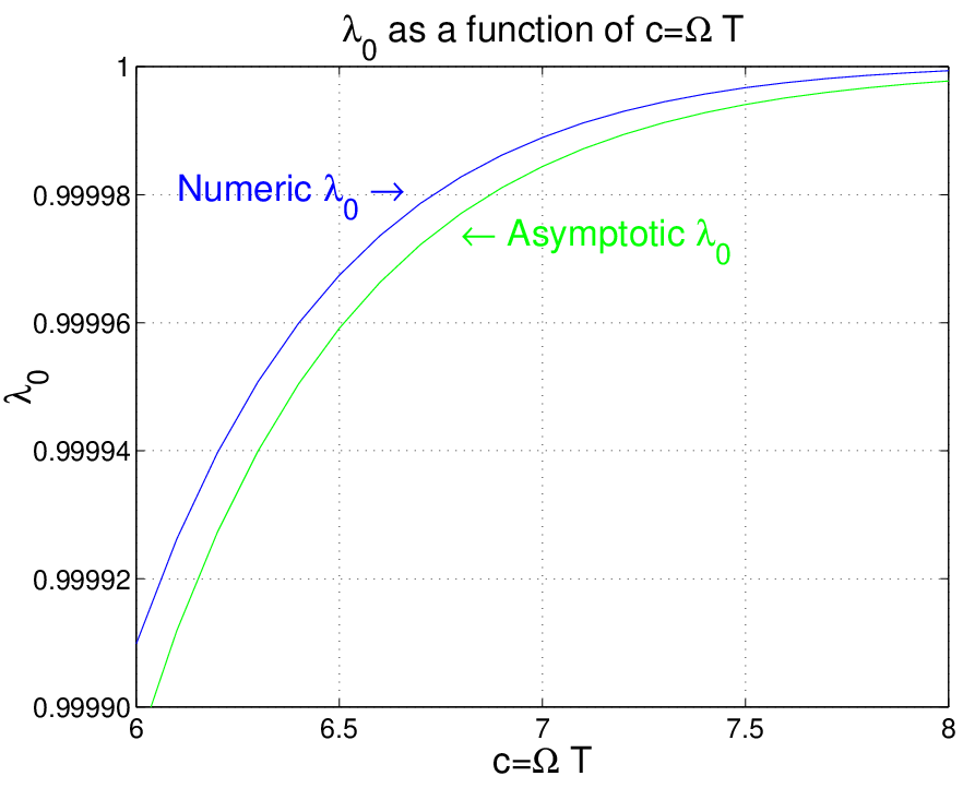
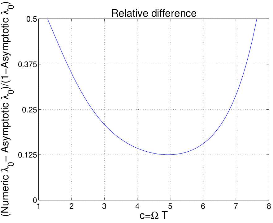
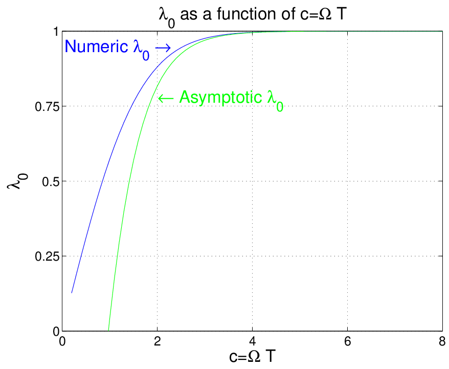
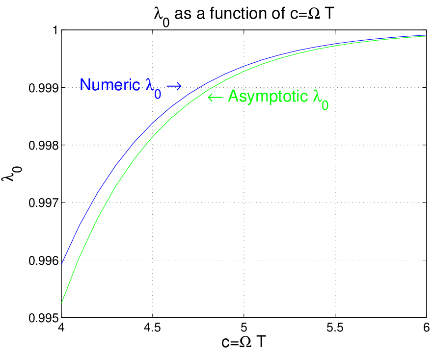
We used H.Xiao, V.Rokhlin and N.Yarvin (XRY) [17] algorithm for computing $\lambda_{0}$ as a function of $c\in[0,6]$ and compered it to the asymptotic formula (6) (see Figure 1). We used $k=300$ for the complexity parameter in XRY [17] algorithm (see equation (54) and section 4 therein) . The asymptotic formula is a good approximation for $\lambda_{0}$ starting from small $c^{\prime}s$. The relative difference (i.e. (Numerical $\lambda_{0}$ - asymptotic $\lambda_{0}$)/(1- asymptotic $\lambda_{0}$)) is decreasing up to $c=5$ and then it starts to increase. We believe that with higher complexity resources then us (We used PC) one should use numerical algorithms for $c\leq 10$. We believe that for $c>10$ the asymptotic formula is good enough.

Possibility maps for different values of $\lambda_{0}$ are plotted in Figure 2. Below we will introduce possibility maps in term of spreading. This is an important difference between our approach to LPS approach.

LP [11] mentioned that their theorem can be used for describing the function $\phi(\alpha,\beta)$ that can be used for writing the uncertainty principle in the form:

or equivalently (to match Figure 2; LP used the concentration parameters $\alpha^{2}_{T}$ and $\beta^{2}_{\Omega}$. We will discuss the parameters issue in section 5):

To the inequalities 7 and 8 above and to their generalizations that will be introduced below we will call Generalized Uncertainty Principles.

LP used the concentrations $\alpha_{T}(f)$ (2) and $\beta_{\Omega}(f)$ (3) for formulating their generalized uncertainty principle. The notion of spreading is in some sense dual to the notion of concentration. In section 4 we will consider uncertainty principles for general weights using the spreading notion and describe the properties of the weights, $w_{1}(x)$ and $w_{2}(\omega)$ (see (11) and (12)), rigourously. In this section we define the time spreading (11) and frequency spreading (12) and use specific weights (9) and (10) that fits to LP Theorem. We will restate LP Theorem, using the spreadings $\gamma(f,a)$ and $\zeta(f,b)$ (see below (11), (12), (9) and (10)). Below we will redefine the terms ”possibility map”, ”possibility body” and ”generalized uncertainty principle” in an obvious way which fits the notion of spreading instead of the notion of concentration. We will use ”the spreading language” from now on.

We define the time weight, $w_{1LP}(x)$, and the frequency weight, $w_{2LP}(\omega)$ as follows:

We define the time spreading function as

and the frequency spreading as

and see that in the case that $w_{1}(x)=w_{1LP}(x)$ and $w_{2}(\omega)=w_{2LP}(\omega)$ we have $\gamma^{2}(f,T)=1-\alpha^{2}_{T}(f)$ and $\zeta^{2}(f,\Omega)=1-\beta^{2}_{\Omega}(f)$.

Therefore, defining $\Psi(\gamma^{2},\zeta^{2})$ and $\psi(\gamma,\zeta)$ on

$D_{LP^{*}}=[0,1]\times[0,1]\setminus\{(0,0),(0,1),(1,0)\}$ by

we get the LP uncertainty principle in the ”spreading language”:

$\Box$

and transforming equation (8) to an equivalent general uncertainty principle in the ”spreading language” we get:

In section 4 we will see that the ”spreading point of view” of LP theorem relates it to HPW uncertainty principle and to general uncertainty principles that are described there. We will redefine some of the terms that we used in the introduction, using the ”spreading language”

We redefine the ”possible area of level c”:

and redefine the ”impossible area of level c”, the complement of $M_{\Omega,T}$ in $D_{LP^{*}}$:

and call the pair $(M_{c},M^{\prime}_{c})$ the possibility map of level c.

We redefine the ”possibility body” by:

Notice that the ”possible areas” in Figure 2 (different $\lambda_{0}$’s corresponds to different $c$’s, see Figure 1) are convex. Analytic derivation of this fact is given below, in the example after Theorem 3.9. To uncertainty inequalities of the form (13),we will call ”Generalized Uncertainty Principle” (we redefined our definition that follows (8) to fit the ”spreading language”).

$\psi$ is a non-increasing function of $\gamma$ for fixed $\zeta$ and a non-increasing function of $\zeta$ for fixed $\gamma$ since $\lambda_{0}(c)$ is an non-decreasing function (see Figure 1)

Now we will derive classical uncertainty principles from the general uncertainty principle of LP.

In Theorem 3.9 above we showed that $M_{c}$, $c>0$ is a non-convex set (we showed that $\zeta$ as a function of $\gamma$ is convex, which is equivalent). We would like to remark that if we use a different set of natural parameters (such as $\zeta^{2}$ and $\gamma^{2}$, see Figure 4) then $M_{c}$, where $c$ belongs to some interval, may be a convex set.

As an example we show that using the parameters $\zeta^{2}$ and $\gamma^{2}$, $M_{c}$, where $\lambda_{0}(c)>\frac{1}{2}$, is a convex set: $M_{c}$ is convex iff $\zeta^{2}$ as a function of $\gamma^{2}$, $0<\gamma^{2}\leq 1-\lambda_{0}$ defined implicitly by $\cos^{-1}\sqrt{1-\gamma^{2}}+\cos^{-1}\sqrt{1-\zeta^{2}}=\cos^{-1}\sqrt{\lambda_{0}}$ is concave. To see that we write $\beta^{2}$ as a function of $\alpha^{2}$

we denote $h(\alpha^{2})=\cos^{-1}\sqrt{\lambda_{0}}-\cos^{-1}\sqrt{\alpha^{2}}$ and differentiate $\beta^{2}(\alpha^{2})$ ($\beta^{2}$ with respect to $\alpha^{2}$ twice) to get

for $\lambda_{0}\geq\frac{1}{2}$ since $sin^{2}(h(\alpha^{2}))\leq\cos^{2}(h(\alpha^{2}))$ and ${(\alpha^{2})}^{\frac{3}{2}}(1-\alpha^{2})^{\frac{1}{2}}\geq{(\alpha^{2})}^{\frac{1}{2}}(1-\alpha^{2})^{\frac{3}{2}}$ we get that $\beta^{2}(\alpha^{2})\leq 0$. $\zeta^{2}(\gamma^{2})$ is concave since $\beta^{2}(\alpha^{2})$ is convex.

One can get different inequalities by minimizing different functions on the possible area. Of course, one can use different coordinates systems to work with for obtaining different inequalities. As an illustration we will use the coordinates $\zeta^{2}$ and $\gamma^{2}$. In this case we will not get a new uncertainty principle. We will get a weaker uncertainty principle then 15, but the illustration is instructive:

From symmetry with respect to the line $\zeta^{2}=\gamma^{2}$ and concavity of the function $\zeta^{2}(\gamma^{2})$, the maximum of the function $\gamma^{2}+\zeta^{2}$ on the possibility map is attained at the point $\gamma^{2}=\zeta^{2}=1-\cos^{2}\frac{\cos^{-1}\sqrt{\lambda_{0}}}{2}$. (We used the equation $2\cos^{-1}\sqrt{1-\gamma^{2}}=\cos^{-1}\sqrt{\lambda_{0}}$).

and we get:

using the identity:

we get the uncertainty principle:

As we mentioned the uncertainty principle (22) is weaker then (15). In fact it is a consequence of (15) using the inequality

Remark: We wanted to point out the convexity of $\zeta(\gamma)$ and the concavity of $\zeta^{2}(\gamma^{2})$. If one is only interested in finding the inequalities, there may be easier ways to get those.

In this section we will generalize the example from section 3 to more general weights. We denote the time weight by $w_{1}(x)$ and the frequency weight by $w_{2}(\omega)$. We will use the notations:

where $a$ is the called the time weight scaling parameter; and

where $b$ is the called the frequency weight scaling parameter. We recall the definitions of time spreading and frequency spreading (see definitions 3.3 and 3.4:

The time spreading:

The frequency spreading:

In section 3 we used specific weights $w_{1LP}(x)$ (see (9)) and $w_{2LP}(\omega)$ (see (10)). In this section we will use general weights that posses mild requirements.

Note that Lemma 4.2 is steal correct if we use a change of coordinates from $R^{4^{+}}$ to $R^{4^{+}}$ of the form $(p,q,a,b)\rightarrow(s(p,q),t(p,q),a,b)$. We will use specific change of variables in Section 5.

Lemma 4.2 indicates that the relevant parameter is the time weight scaling parameter $\times$ the frequency weight scaling parameter; So, we can define realizable points in $R^{3+}$ instead of in $R^{4+}$:

Note that we may think of the set $PB_{\gamma^{1},\zeta^{1}}$ as the set:

where we identify points such that $ab=c$.

The meaning of the subindexes will be clear in Section 5, since definitions 4.1, 4.3 and 4.4 are special cases of the more general definitions 5.1, 5.2 and 5.3 in section 5. In the following it also will become clear that the possibility body PB defined in Definition 3.8. is similar to $PB_{\gamma^{1},\zeta^{1}}$ when we use LP-weights (9) and (10).

We will use the following type of weights in the theorem. The weights in LP result , (9) and (10), are pointwise limit of weights of type 1.

Restricting ourselves to weights of type 1 we get the following generalized uncertainty principle:

References

• [1] C.J. Bouwkamp: On spheroidal wave functions of order zero, J.Math. Phys. Mass. Inst. Tech 26 79-92 (1947).
• [2] D.L.Donoho, P.B.Stark, Uncertainty principles and signal recovery, SIAM J. Appl. Math, 49, 906-931 (1989)
• [3] W.H.J.Fuchs, On the Eigenvalues of an Integral Equation Arising in the Theory of Band-Limited Signals, J. Math. Anal. Appl. 9 (1964), 317-330.
• [4] G.B. Folland, A. Sitaram, ”The uncertainty principle: A mathematical survey”, The Jornal of Fourier Analysis and Applications, volume 3, number 3, 1997.
• [5] D. Gabor, Theory of communication, J.IEE, 93, 429-457 (1946)
• [6] K. Grochening, Foundations of Time-Frequency Analysis, Birkhauser (2000)
• [7] W. Heisenberg (1927) U¨\ddot{U}ber den anschaulichen Inhalt der quantentheoretischen Kinematic und Mechanik. Zeit. Physik 43. 172-198.
• [8] A. Karoui, T. Moumni, New efficient methods for computing the prolate spheroidal wave functions and their corresponding eigenvalues
• [9] K. Khare, N. George, Sampling theory approach to prolate spheroidal wave functions, J. Phys. A 36 (2003) 10011-10021.
• [10] E.H. Kennard, Zur Quantenmechanik einfacher Bewegungstypen. Zeit. Physik 44, 326-352 (1927).
• [11] H.J. Landau, H.O. Pollak, Prolate spheroidal wave functions, Fourier analysis and uncertainty - II, Bell Syst. Tech. J., 40,65-84 (1961)
• [12] H.J. Landau, H.O. Pollak, Prolate spheroidal wave functions, Fourier analysis and uncertainty - III: The dimension of the space of essentially time and band limited signals, Bell Syst. Tech. J., July 1962, pages: 1295-1336
• [13] D. Slepian, H.O. Pollak, Prolate spheroidal wave functions, Fourier analysis and uncertainty - I, Bell Syst. Tech. J.,40, 43-64 (1961).
• [14] V. Palamodov, Degree of freedom of fields concentrated in a compact domain, preprint 2006
• [15] E.C. Titchmarsh, Eigenfunction expansions associated with second order differential equations, part II; Oxford At The Clarendon Press 1958.
• [16] H. Weyl (1928). Gruppentheorie und Quantenmechanik. S.Hirzel, Leipzig. Revised English edition: The Theory of Groups and Quantum Mechanics Methuen, Lomdon, 1931; reprinted by Dover, New York, 1950.
• [17] H. Xiao, V. Rokhlin, N. Yarvin, Prolate spheroidal wavefunctions, quadrature and interpolation; Inverse Problems 17 (2001) 805-838