Single-Field Inflation After WMAP5
Abstract
Single-field models of inflation are analysed in light of the WMAP five-year data. Assuming instantaneous reheating, we find that modular/new inflation models with small powers in the effective inflaton self-interaction are more strongly constrained than previously. The model with a cubic power lies outside the regime when the number of e-folds is . We also find that the predictions for the intermediate model of inflation do not overlap the region regardless of the power of the monomial potential. We analyse a number of ultra-violet, DBI braneworld scenarios involving both wrapped and multiple-brane configurations, where the inflaton kinetic energy is close to the maximum allowed by the warped geometry. In all cases, we find that the parameters of the warped throat are strongly constrained by observations.
pacs
98.80.CqI Introduction
The inflationary scenario postulates that the universe underwent a phase of very rapid, accelerated expansion in its distant past. Observations – most notably from the anisotropy power spectrum of the Cosmic Microwave Background (CMB) – have provided strong support for the paradigm. Despite this success, however, the mechanism which drove the inflationary expansion has yet to be identified. Indeed, there remain many viable versions of the scenario. (For reviews, see, e.g., Refs. [1, 2, 3, 4, 5, 6, 7, 8].) In view of this, it is important to constrain, and ultimately rule out, as many models of inflation as possible.
In this paper, we consider a wide range of inflationary models that are well motivated from particle physics and unified field theory. We focus on models where the cosmic expansion was driven by a single, self-interacting scalar ‘inflaton’ field, . In general, single-field inflationary models are characterised by the action
| (1) |
where is the Ricci curvature scalar, the ‘kinetic function’ is a function of the inflaton field and its kinetic energy , and is the reduced Planck mass. In the simplest versions of the scenario, the inflaton has a canonically normalised kinetic energy, where and denotes the inflaton potential. In many higher-dimensional models motivated directly from string/M-theory, however, the function has a more complicated form. This is the case, for example, in the Dirac-Born-Infeld (DBI) inflationary scenario, where inflation is driven by the propagation of one or more -branes [9].
We compare both canonical and non-canonical models of inflation with the recent observational bounds derived from the combined data of the Wilkinson Microwave Anisotropy Probe (WMAP) [10], Baryon Acoustic Oscillations (BAO) [11] and Supernovae (SN) surveys [12, 13, 14, 15]. In Ref. [16], the three-year WMAP data was employed to rule out for the first time a large fraction of viable canonical models at more than . We begin by reconsidering this analysis in the light of the WMAP five-year data [10]. We find that the conclusions of [16] are confirmed by WMAP5, with the improved bounds on the scalar spectral index strongly constraining models of modular inflation at more than the 2 level.
We then proceed to consider non-canonical DBI brane inflationary models driven by a wrapped - or -brane [9, 17, 18]. We focus on the ‘relativistic, ultra-violet’ version of the scenario, where the brane is moving towards the tipped region of a warped throat with a kinetic energy close to the upper bound imposed by the warpfactor of the higher-dimensional space. We find that independently of the form of the inflaton potential, the geometry of the warped throat must be strongly constrained if such models are to satisfy the improved observational bounds from WMAP5. We also consider extensions of the scenario to multiple-brane configurations [19, 20] and find that the same challenges arise as for the single-brane case.
The structure of the paper is as follows. In section II, we summarise the current bounds on the observational parameters. In section III, we investigate models of canonical inflation and determine which models are still viable. In Sections IV and V, we derive new observational limits on wrapped and multi-brane UV DBI inflation. We conclude with a discussion in Section VI.
II Single-Field Inflation
For the action (1), the amplitudes of the scalar and tensor perturbation spectra generated during inflation are given by [21]
| (2) |
respectively, where , the sound speed of inflaton fluctuations is defined by
| (3) |
and a comma denotes partial differentiation. The corresponding spectral indices are given by
| (4) |
and the tensor-scalar ratio, , is
| (5) |
In canonical inflation the sound speed of inflaton fluctuations is equal to the speed of light, . The scalar spectral index is therefore determined by
| (6) |
where
| (7) |
represent the ‘slow-roll’ parameters and a prime denotes . Successful slow-roll inflation requires a sufficiently flat potential, .
The observed normalisation of the CMB anisotropy power spectrum implies that . If it is assumed that the scalar spectral index is effectively constant over observable scales and that is negligible, the WMAP5 data [10] indicates that
| (8) |
at the confidence level. Combining WMAP5 with the BAO and SN data reduces the uncertainty in the matter density and results in an improved bound on when the tensor-to-scalar ratio is included [10]. To be consistent we also use the bounds from this data set in the case where is negligible:
| (9) |
It is important to note that even if the tensor-scalar ratio is significant, the Harrison-Zeldovich spectrum is still highly disfavoured. On the other hand, if the running of the spectral index, , is treated as a free parameter, would be consistent with the data. The upper limit on the tensor-scalar ratio from the combined data is at the level when is assumed as a prior. This is relaxed to for .
Deviations from Gaussian statistics in the scalar perturbation spectrum are quantified in terms of the ‘non-linearity’ parameter, . In the equilateral triangle limit, where the three momenta have equal magnitude, the leading-order contribution to this quantity is determined by the kinetic function and its first three derivatives [22, 23, 24]:
| (10) |
where
| (11) |
Current limits on the non-linearity parameter are at the level [10].
Finally, the number of e-folds of canonical, slow-roll inflation that occurred from the time when observable scales first crossed the Hubble radius during inflation to the epoch when inflation ended is given by
| (12) |
The value of depends on the reheating temperature. Requiring baryogenesis to take place at or above the electroweak scale implies that . A value of corresponds to a GUT scale reheating and hence an instantaneous change from inflation to relativistic matter domination.
III Canonical Inflation
In order to decide whether a particular model is favoured by the data or not we implicitly make the following assumptions in this Section:
- 1.
The curvature perturbation was sourced entirely from quantum fluctuations in a single, slowly rolling scalar inflaton field and is purely adiabatic. We work to leading-order in the slow-roll approximation.
- 2.
The running in the spectral index vanishes11 1 This is a reasonable prior since the latest WMAP analysis concludes that there is no support from the data to treat the running as a free parameter [10]., .
- 3.
The form of the potential under study remains valid until the end of inflation.
- 4.
The universe reheats instantaneously immediately after the end of inflation.
- 5.
Assuming instantaneous reheating, a reasonable range of values for the number of e-folds between and is taken to be , in accordance with the literature and more specifically Ref. [25]. (We note, however, that the number of e-folds could lie outside this region in either direction if further assumptions are made).
In the following, therefore, when a model is said to be ‘excluded convincingly at more than a given confidence limit for a given value of ’, this should be understood within the context of the above assumptions.
III.1 Small-Field Canonical Inflation
Small-field models are defined as those for which the variation in the inflaton field is less than the reduced Planck mass, . Typically, the amplitude of gravitational waves generated in such models is undetectably small and the spectral index therefore provides the key observational discriminator.
A general form for the small-field inflaton potential is given by
| (13) |
where are constants. When is an integer and greater than 2, such a potential may be generated by the self-coupling of the inflaton at tree-level. A potential of this form also arises in the new [26, 27, 28] and modular inflationary scenarios [29, 30]. The mutated hybrid models correspond to the ranges or , where is not necessarily an integer [31]. The case corresponds to certain braneworld models, where the constant term arises from the warped tension of the brane and anti-brane and the interaction term originates from the attraction between the branes [32, 33].
Another small-field model of interest is the supersymmetric (SUSY) -term potential resulting from one-loop corrections of the waterfall field in SUSY hybrid inflation [34, 35, 36]. In this scenario, supersymmetry is broken spontaneously and the potential has the form
| (14) |
where and are model-dependent parameters.
Finally, we consider the potential
| (15) |
with , which may be generated when the flat direction in SUSY is lifted by adding a Kahler potential, i.e., by adding kinetic terms [36]. (Note, however, that this is not a small-field model as defined above, since in the region where dominates.)
All the above models are related through their observational predictions for the value of the spectral index. For both the potentials (14) and (15), the slow-roll parameter dominates over during inflation. However, this is only true for the potential (13) in the small-field regime and we therefore implicitly assume22 2 One could consider cases where , but this would correspond to a large-field model, and would result in a larger tensor fraction for which equation (16) would not apply [37]. that . The fact that implies that the spectral index is given by and, since is a continuously increasing function of during inflation, this expression can be combined with the number of e-folds, Eq. (12), to deduce a general form for the spectral index [38, 2]:
| (16) |
In Eq. (16), the SUSY F-term hybrid model (14) corresponds formally to and the potential (15) to the value .
In Figs. 1-3, we explore the regions of parameter space defined by that are consistent with the observations. In all cases, the bound (9) on the spectral index is employed. In Fig. 1, the number of e-folds, , is treated as an independent variable and the spectral index, , is varied. The relation (16) is plotted for a range of values for . In Fig. 2, the parameter is varied with respect to for a fixed . The bounds (9) are highlighted to emphasise the allowed regions of parameter space. Finally, in Fig. 3, the value of is varied with respect to the spectral index for fixed values of the number of e-folds in the range .


| Outside the | Outside the | |
| region | region | |
In [16], the original hybrid inflation model was excluded convincingly at more than . This is still the case with the new data sets. On the other hand, the (mutated hybrid) and (exponential) models fit the data well for the reasonable range of . Within the context of the present discussion, the key features of the new data are the increase in the central value of the spectral index and the narrowing of the error bars. As a result, the model of the new and modular inflationary scenarios is now outside the region for , as can be seen from Fig. 1. Referring to Fig. (3) and considering positive values of , we find that is required for inclusion at the level if , whereas is necessary if . Moreover, for inclusion at , these limits strengthen to if and if . The exclusion limits for various values of are summarised in Table 1.
The fact that it is the lower-order terms that are constrained by the data is important from the theoretical point of view, because it is difficult to motivate the suppression of lower-order terms in a small-field theory. Such a suppression requires either a significant fine-tuning of the coupling terms or the introduction of a suitable symmetry. The problem of suppressing the quadratic term in modular inflation was addressed in Ref. [39], where a symmetry was identified. However, the majority of model builders prefer to impose fine-tuning to suppress this term [40] and this emphasises the difficulty of constructing a small-field model of inflation where a higher-order term is responsible for inflation coming to an end. This is an important open question that needs to be addressed.
III.2 Large-Field Canonical Inflation
Large-field models are characterised by the condition . They are particularly interesting since a super-Planckian field variation may generate an observable tensor-scalar ratio [41]. The simplest class of large-field models is based on a monomial potential, , where is a positive [42] or negative [43, 44, 45] constant. The former case corresponds to chaotic inflation, whereas the latter corresponds to the intermediate inflationary scenario which was analysed in light of the WMAP3 data in Ref. [46]. Assuming that the potential maintains this form up to the end of inflation, the generic predictions for this class of models are:
| (17) |
for , and
| (18) |
for .

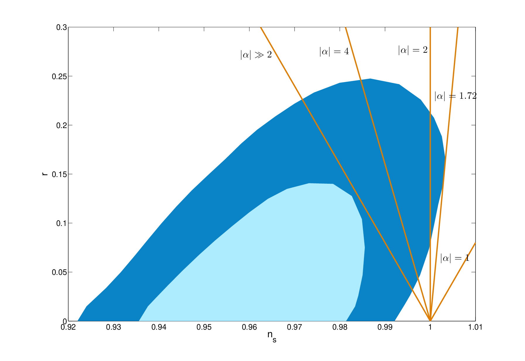
Since the predictions of a particular model are sensitive to the number of e-folds that elapsed between observable scales leaving the horizon and the end of inflation, we have plotted Eq. (17) for different values of in Fig. 4. On each line we have identified the predictions for specific values of in the range . We note that for potentials with , is required in order for the predictions to lie inside the contour.
It is interesting to consider what one might be able to deduce from the plane in the near future with regard to concave-downwards potentials , especially given the anticipated results from the Planck surveyor. This class of models is of relevance to braneworld inflation within the context of type IIA string theory compactified on a six-dimensional, bulk space that is comprised of two nil-manifolds [47]. Depending on the direction in which the brane moves, the leading-order term in the effective inflaton potential is a monomial with or .
The Planck surveyor is expected to be sensitive to a primordial gravitational wave background of , as shown by the horizontal dashed line in Fig. 4. For illustrative purposes, let us suppose that the allowed range of values for deduced from the Planck data at a given confidence level turns out to be similar to that from WMAP5 with the same set of priors33 3 Naturally, we do not expect it to be the same. The purpose of this discussion is to illustrate how the method could be employed in practice when the data is made available.. In that case, Fig. 4 indicates that a tensor background would not be detectable for when the number of e-folds is in the range , but could be for , for example. The model, on the other hand, predicts that for all .
Finally, we consider the implications of WMAP5 for the intermediate inflationary scenario. Rearanging Eq. (18) implies that [46]
| (19) |
and Eq. (19) is plotted in Fig. 5 for various values of . It should be noted that this model leads to eternal inflation and some hybrid mechanism is therefore required in order to bring inflation to an end. In this sense, the value of the inflaton field at the end of inflation is unspecified and, consequently, any value for is possible in principle. Nonetheless, we deduce that in the limit . This limit is shown in Fig. 5 and does not intersect the 1 region. For this particular combination of data sets, therefore, the intermediate scenario lies outside the contour for all values of and all models with lie outside the regime.
IV Inflation with Wrapped Branes
The DBI inflationary scenario is based on the compactification of type IIB string theory on a Calabi-Yau (CY) three-fold [9]. Non-trivial form-field fluxes generate warped ‘throat’ regions within the CY space and inflation arises when a D-brane propagates inside such a throat. The inflaton parametrises the radial position of the brane and, since this is an open string mode, its dynamics is determined by a DBI action.
In general, the metric inside the throat has the form , where the warpfactor is a function of the radial coordinate along the throat and the base is an Einstein-Sasaki manifold. When the throat geometry is , the warpfactor is , where defines the radius, represents the -brane charge on the cone, is the dimensionless volume of the base with unit radius, and and denote the string mass and coupling, respectively.
A well-motivated exact warped geometry is provided by the Klebanov-Strassler (KS) background, where the base is with [48]. Moreover, in the F-theory interpretation of type IIB compactifications, the global tadpole cancellation relates the background charge to the Euler characteristic, , of the CY four-fold such that [49]. For the case of four-fold manifolds that are known explicitly, , which implies that [50].
In the original version of the scenario, inflation was driven by the motion of a -brane [9]. However, this model is inconsistent with the data if is large [51, 52, 53, 54]. Recently, extended versions involving - and -branes wrapped over cycles of the throat have been considered [17, 18]. The key difference between these models is the relationship between the inflaton field and the radial coordinate. When the NS-NS two-form potential vanishes this is given by
| (20) |
for an throat, where we denote the -brane by the subscript , defines the brane tension and represents the wrapped volume. (Note that .)
The effective four-dimensional action for the brane dynamics is then given by Eq. (1) with a kinetic function [17, 18]:
| (21) |
where the warped brane tension is defined by
| (22) |
The warped nature of the geometry imposes an upper limit on the inflaton’s kinetic energy. In this and the following Section, we consider the ‘relativistic, ultra-violet’ DBI scenario, where this upper limit is saturated, , and the brane is moving towards the tip of the throat, . We do not specify the form of the inflaton potential (subject to the condition that a phase of quasi-exponential expansion is generated). It follows that
| (23) |
Moreover, the scalar perturbation amplitude has the form
| (24) |
and, since , the non-linearity parameter is given by [24, 55].
The observable parameters in this scenario are , whereas the key parameters describing the warped throat are . Our aim is to constrain these parameters with the WMAP5 data in a way that is independent of the inflaton potential. We proceed by substituting Eq. (23) into the scalar perturbation amplitude to deduce that
| (25) |
Assuming a quasi-de Sitter expansion, we differentiate Eq. (25) with respect to the comoving wavenumber, [21, 52, 53]. Substituting Eqs. (5) and (25) into the result then yields a constraint equation involving the spectral index:
| (26) |
where we have defined the quantity
| (27) | |||||
The left-hand side of Eq. (26) is determined entirely by observable quantities, whereas the right-hand side depends on field-theoretic parameters. Since WMAP5 strongly favours a red perturbation spectrum () [10], Eq. (26) yields the upper limit
| (28) |
once current observational bounds are imposed. It follows, therefore, that rearranging Eq. (27) in the form
| (29) |
leads to an observational upper limit on the ratio . Invoking the canonical values and for the wrapped volumes, respectively, we find that
| (30) |
With a typical value of , the ratio for all currently known CY four-folds. We may conclude, therefore, that consistency with the data for both the wrapped 5- and 7-brane models would require either a smaller than expected value for the base volume or the discovery of new classes of CY four-folds with a larger Euler number.
The theoretic lower bound on can be reduced by allowing the brane to wind around the cycle of the throat or by wrapping it around a base that is orbifolded. For example, if a -brane has a winding number and wraps around a cycle of that is orbifolded by , the normalisation is altered by a factor of [17]. This modifies the value of the parameter defined in Eq. (23) by a factor and, consequently, the value of by . It follows, therefore, that the upper bound (30) for the scenario becomes
| (31) |
This implies that a large amount of winding or orbifolding is required.
It is interesting to consider how the constraints (30) compare to previously known bounds in the light of the WMAP5 data. There exists a field-theoretic upper bound on the tensor-scalar ratio in these scenarios, which arises because the warped nature of the bulk manifold restricts the maximally allowed variation in the value of the inflaton field [56, 51]. For the and models, this constraint was recently expressed in terms of the upper bound [18]
| (32) |
Comparison with Eq. (27) implies that this constraint can be expressed succinctly in the form
| (33) |
The WMAP3 data imposed the limits and at the level, which implies that the upper bound (28) would have been . This is comparable in strength to the theoretic bound (33). Indeed, prior to the WMAP5 data, the wrapped -brane scenario was still compatible with such a limit if and [18]. However, the WMAP5 data has strengthened the bound (30) on by a factor of with the result that all wrapped versions of the scenario now face theoretical challenges if they are to be consistent with the observations.
It is also interesting to note that post WMAP5, the limit (31) is comparable numerically to a corresponding limit for the ratio derived in Ref. [17]. (The limit (31) would have been weaker by a factor of approximately if the WMAP3 data had been employed). However, the analysis of Ref. [17] was restricted to the specific case of a quadratic potential and did not consider the observational constraints on the spectral index. Since the above analysis was independent of the potential, this indicates that any modifications to are unlikely to significantly weaken the upper limit on .
In conclusion, therefore, one of the consequences of the WMAP5 data is that the strongest constraints on the wrapped, relativistic, UV DBI inflationary scenario now arise from the observable plane. On the other hand, it is important to note that backreaction effects are more significant in the wrapped scenarios when the brane is moving relativistically [17, 57]. Consequently, a more detailed analysis of such effects is required before these models can be concretely excluded. Nonetheless, it is known that a wrapped -brane with flux is dual to coincident -branes in the large limit [58]. In view of this, we proceed in the next Section to consider inflation from multiple-brane configurations.
V Inflation with Multiple Branes
In general, the theory of multiple-brane configurations is non-Abelian since coincident branes have open string degrees of freedom which combine to fill out representations of . Recently, the effective action for coincident -branes was derived in the finite limit by employing an iterative technique based on the fundamental representation of and taking an appropriate symmetrized trace over the gauge group [19, 20]. It was found that for all values of , the kinetic function has the form
| (34) |
in the ‘relativistic’ limit , where is defined by
| (35) |
It was further shown that backreaction effects are kept under control for sufficiently small values of [20].
We consider the relativistic, UV DBI scenario, where the branes are moving down an throat such that and . The parameter therefore takes a constant value. It follows from Eqs. (3) and (34) that the non-linearity parameter is related to the sound speed of the inflaton fluctuations by [20]. It can be further shown that the scalar perturbation amplitude for this multi-brane scenario is given by [20]
| (36) |
In principle, this scenario could be constrained observationally by deriving the analogue of Eq. (26). However, the dependence of the scalar perturbation amplitude on the non-linearity parameter introduces an additional term involving the running . Although this parameter might be detectable in future experiments, there is presently no data available to constrain it. To proceed, therefore, we need to invoke a further assumption by specifying the form of the potential. In general, a mass term is expected to be generated below a critical scale due to the breaking of conformal invariance. We therefore consider a quadratic potential, .
To generate a phase of quasi-exponential expansion, , the inflaton potential must dominate the energy density. In this case, the Friedmann equation reduces to and it follows that
| (37) |
The consistency equation (5) then implies that the scalar perturbation amplitude varies as . Differentiating with respect to comoving wavenumber therefore implies that
| (38) |
and we may deduce immediately that this model predicts a red perturbation spectrum, as favoured by the WMAP5 data.
The ratio can be constrained by substituting Eqs. (35) and (37) into Eq. (36). We find that
| (39) |
and it follows from the consistency equation (38) that
| (40) |
Imposing current WMAP5 upper limits on the observable parameters then implies that
| (41) |
We conclude, therefore, that when confronted with the observations, the multi-brane scenario (with a quadratic inflaton potential) faces the same theoretical challenges as the single, wrapped configurations: either a new class of CY four-fold is required or the base manifold must be orbifolded.
On the other hand, despite such issues, it is interesting to note that the multi-brane scenario predicts a strong lower limit on the tensor-scalar ratio. Since at the 1 level, Eq. (38) implies that , where we have saturated the WMAP5 bound in the lower limit. This implies that the prospects for detecting primordial gravitational waves from this model with future space-based, all-sky CMB polarisation experiments are good. Moreover, Eq. (5) may be expressed in terms of observable parameters such that . As shown in Ref. [55], deviations of this form from the standard inflationary consistency equation, , could be detected in future CMB surveys if . Substituting this limit into Eq. (38) therefore implies that such a detection could be possible if . This would provide a powerful observational discriminant for breaking the degeneracy between canonical and non-canonical, single-field inflation.
VI Discussion
In this paper, we have considered the status of a wide class of single-field inflationary models in the light of the recent WMAP5 data. For the reasonable range of e-fold values aforementioned, , we conclude that modular/new inflation models with are under pressure from the data and that and satisfy the observations. The required suppression of lower-order terms in the models poses a challenge to model builders, as discussed in Section III. Moreover, it is significant that independent data sets are now converging towards a preferred value of , with only tiny differences between WMAP5 only, [59] and data. This convergence implies that we can be more confident as to what represents a viable model from a phenomenological point of view.
We have also shown that the intermediate inflationary scenario can only satisfy the data at for , and that the predictions of the model do not overlap the region for any value of .
We emphasize that the above conclusions follow from assuming that the reheating of the universe immediately after inflation was instantaneous. However, the precise duration of the reheating process is not known. In particular, for a quadratic potential, a matter dominated phase may arise if the inflaton oscillates about its potential minimum for an extended interval before decaying. This would alter the number of e-folds that elapsed from the epoch when observable scales first crossed the Hubble radius during inflation to the time when inflation ended. In general, the number of e-folds depends on the effective equation of state after inflation and this would need to be known if a more precise value of is to be determined.
Complementary to our work is that of Ref. [60], where the authors start from the different stand point of aiming to construct the most general inflationary potential using slow-roll reconstruction with a specific e-fold and reheat temperature prior. Reconstructing the inflationary slow-roll parameters and not the spectral parameters from the data has the advantage of directly probing more fundamental parameters. They locate regions in space which are consistent with the WMAP5 data, and this allows to reconstruct the Hubble parameters and therefore (via the Hamilton-Jacobi equations) the inflationary potential. The authors also analyse higher-order parameters, but for the purposes of this work, we only need mention that the simplest fit is consistent with the crucial prior of , which we interpret as support for the inflationary paradigm.
We have also considered the relativistic, ultra-violet, DBI braneworld scenario, where the inflaton is identified in terms of the radial position of a wrapped - or -brane. We found that when the brane’s kinetic energy is maximised, new constraints on the parameters of the bulk geometry can be derived from the WMAP5 data in the plane. Such constraints are independent of the precise form of the inflaton potential and are stronger than existing limits originating from field-theoretic bounds on the tensor-scalar ratio. In all cases, consistency with the data requires a significant reduction in the volume of the base or the discovery of new classes of Calabi-Yau four-folds which allow for larger Euler numbers.
We then extended our analysis to a recently proposed relativistic, multi-brane DBI scenario. For the case where the inflaton has a quadratic potential, we found that the predicted value of the spectral index is compatible with observations. However, the ratio is still strongly bounded from above, as in the single brane models, and consequently the same theoretical problems arise in this case also.
VII Acknowledgements
We thank D. Lyth and K. Malik for helpful discussions. We acknowledge use of the Cosmomc Matlab scripts. LA is supported by the Science and Technologies Facilities Council (STFC) under Grant PP/E001440/1.
References
- [1] D. H. Lyth and A. Riotto, Phys. Rept. 314, 1 (1999), eprint hep-ph/9807278.
- [2] A. R. Liddle and D. H. Lyth, Cosmological inflation and large-scale structure (Cambridge, UK: Univ. Pr. 400 p, 2000).
- [3] A. H. Guth and D. I. Kaiser, Science. 307, 884 (2005), eprint astro-ph/0502328.
- [4] J. M. Cline (2006), eprint hep-th/0612129.
- [5] S. H. Henry Tye, Lect. Notes Phys. 737, 949 (2008), eprint hep-th/0610221.
- [6] L. McAllister and E. Silverstein, Gen. Rel. Grav. 40, 565 (2008), eprint 0710.2951.
- [7] A. Linde, Lect. Notes Phys. 738, 1 (2008), eprint 0705.0164.
- [8] D. H. Lyth, Lect. Notes Phys. 738, 81 (2008), eprint hep-th/0702128.
- [9] M. Alishahiha, E. Silverstein, and D. Tong, Phys. Rev. D70, 123505 (2004), eprint hep-th/0404084.
- [10] E. Komatsu et al. (WMAP) (2008), eprint arXiv:0803.0547 [astro-ph].
- [11] W. J. Percival et al., Mon. Not. Roy. Astron. Soc. 381, 1053 (2007a), eprint 0705.3323.
- [12] A. G. Riess et al. (Supernova Search Team), Astrophys. J. 607, 665 (2004), eprint astro-ph/0402512.
- [13] P. Astier et al. (The SNLS), Astron. Astrophys. 447, 31 (2006), eprint astro-ph/0510447.
- [14] A. G. Riess et al., Astrophys. J. 659, 98 (2007), eprint astro-ph/0611572.
- [15] W. M. Wood-Vasey et al. (ESSENCE), Astrophys. J. 666, 694 (2007), eprint astro-ph/0701041.
- [16] L. Alabidi and D. H. Lyth, JCAP 0608, 013 (2006), eprint astro-ph/0603539.
- [17] M. Becker, L. Leblond, and S. E. Shandera, Phys. Rev. D76, 123516 (2007), eprint 0709.1170.
- [18] T. Kobayashi, S. Mukohyama, and S. Kinoshita, JCAP 0801, 028 (2008), eprint 0708.4285.
- [19] S. Thomas and J. Ward, Phys. Rev. D76, 023509 (2007), eprint hep-th/0702229.
- [20] I. Huston, J. E. Lidsey, S. Thomas, and J. Ward, JCAP 0805, 016 (2008), eprint 0802.0398.
- [21] J. Garriga and V. F. Mukhanov, Phys. Lett. B458, 219 (1999), eprint hep-th/9904176.
- [22] J. M. Maldacena, JHEP 05, 013 (2003), eprint astro-ph/0210603.
- [23] D. Seery and J. E. Lidsey, JCAP 0506, 003 (2005), eprint astro-ph/0503692.
- [24] X. Chen, M.-x. Huang, S. Kachru, and G. Shiu, JCAP 0701, 002 (2007), eprint hep-th/0605045.
- [25] A. R. Liddle and S. M. Leach, Phys. Rev. D68, 103503 (2003), eprint astro-ph/0305263.
- [26] A. D. Linde, Phys. Lett. B108, 389 (1982).
- [27] A. Albrecht and P. J. Steinhardt, Phys. Rev. Lett. 48, 1220 (1982).
- [28] T. Banks, M. Berkooz, S. H. Shenker, G. W. Moore, and P. J. Steinhardt, Phys. Rev. D52, 3548 (1995), eprint hep-th/9503114.
- [29] A. D. Linde, Phys. Lett. B132, 317 (1983a).
- [30] P. Binetruy and M. K. Gaillard, Phys. Rev. D34, 3069 (1986).
- [31] E. D. Stewart, Phys. Lett. B345, 414 (1995a), eprint astro-ph/9407040.
- [32] G. R. Dvali and S. H. H. Tye, Phys. Lett. B450, 72 (1999), eprint hep-ph/9812483.
- [33] S. Kachru, R. Kallosh, A. Linde, and S. P. Trivedi, Phys. Rev. D68, 046005 (2003), eprint hep-th/0301240.
- [34] E. J. Copeland, A. R. Liddle, D. H. Lyth, E. D. Stewart, and D. Wands, Phys. Rev. D49, 6410 (1994), eprint astro-ph/9401011.
- [35] G. R. Dvali, Q. Shafi, and R. K. Schaefer, Phys. Rev. Lett. 73, 1886 (1994), eprint hep-ph/9406319.
- [36] E. D. Stewart, Phys. Rev. D51, 6847 (1995b), eprint hep-ph/9405389.
- [37] J. Martin and C. Ringeval, JCAP 0608, 009 (2006), eprint astro-ph/0605367.
- [38] W. H. Kinney and K. T. Mahanthappa, Phys. Rev. D53, 5455 (1996), eprint hep-ph/9512241.
- [39] G. G. Ross and S. Sarkar, Nucl. Phys. B461, 597 (1996), eprint hep-ph/9506283.
- [40] Z. Lalak, G. G. Ross, and S. Sarkar (2005), eprint hep-th/0503178.
- [41] D. H. Lyth, Phys. Rev. Lett. 78, 1861 (1997), eprint hep-ph/9606387.
- [42] A. D. Linde, Phys. Lett. B129, 177 (1983b).
- [43] J. D. Barrow, Phys. Lett. B235, 40 (1990).
- [44] J. D. Barrow and P. Saich, Phys. Lett. B249, 406 (1990).
- [45] A. G. Muslimov, Class. Quant. Grav. 7, 231 (1990).
- [46] J. D. Barrow, A. R. Liddle, and C. Pahud, Phys. Rev. D74, 127305 (2006), eprint astro-ph/0610807.
- [47] E. Silverstein and A. Westphal (2008), eprint arXiv:0803.3085 [hep-th].
- [48] I. R. Klebanov and M. J. Strassler, JHEP 08, 052 (2000), eprint hep-th/0007191.
- [49] S. Sethi, C. Vafa, and E. Witten, Nucl. Phys. B480, 213 (1996), eprint hep-th/9606122.
- [50] A. Klemm, B. Lian, S. S. Roan, and S. T. Yau, Nucl. Phys. B518, 515 (1998), eprint hep-th/9701023.
- [51] J. E. Lidsey and I. Huston, JCAP 0707, 002 (2007), eprint arXiv:0705.0240 [hep-th].
- [52] H. V. Peiris, D. Baumann, B. Friedman, and A. Cooray, Phys. Rev. D76, 103517 (2007), eprint 0706.1240.
- [53] R. Bean, S. E. Shandera, S. H. Henry Tye, and J. Xu, JCAP 0705, 004 (2007), eprint hep-th/0702107.
- [54] L. Lorenz, J. Martin, and C. Ringeval, JCAP 0804, 001 (2008), eprint 0709.3758.
- [55] J. E. Lidsey and D. Seery, Phys. Rev. D75, 043505 (2007), eprint astro-ph/0610398.
- [56] D. Baumann and L. McAllister, Phys. Rev. D75, 123508 (2007), eprint hep-th/0610285.
- [57] R. Bean, X. Chen, H. V. Peiris, and J. Xu, Phys. Rev. D77, 023527 (2008), eprint 0710.1812.
- [58] J. Ward, JHEP 12, 045 (2007), eprint arXiv:0711.0760 [hep-th].
- [59] W. J. Percival et al., Astrophys. J. 657, 645 (2007b), eprint astro-ph/0608636.
- [60] H. V. Peiris and R. Easther (2008), eprint 0805.2154.