-matrix and Quantum Tunneling
in Gravitational
Collapse
Abstract
Using the recently introduced ACV reduced-action approach to transplanckian scattering of light particles, we show that the -matrix in the region of classical gravitational collapse is related to a tunneling amplitude in an effective field space. We understand in this way the role of both real and complex field solutions, the choice of the physical ones, the absorption of the elastic channel associated to inelastic multigraviton production and the occurrence of extra absorption below the critical impact parameter. We are also able to compute a class of quantum corrections to the original semiclassical -matrix that we argue to be qualitatively sensible and which, generally speaking, tend to smooth out the semiclassical results.
DFF 446/07/08
1 Introduction
In a recent paper [1], Amati, Veneziano and one of us have proposed a simplified approach to the -matrix for transplanckian scattering of light particles which could possibly describe the region of classical gravitational collapse. This treatment originates from the eikonal approach to high-energy string-gravity proposed in the eighties [2] and resums a class of corrections to the leading eikonal operator which correspond to tree diagrams generated by some effective high-energy graviton emission vertices.
The simplified action approach [1] is valid in a high energy regime () in which the gravitational radius and the impact parameter of the light scattering particles are large w.r.t. the string length , so that string effects are normally negligible. Thus, the dynamical variables are basically metric fields which, due to the high-energy kinematics, are integrated over longitudinal space () and follow a reduced dynamics in transverse space, which is two-dimensional for . The reduced two-dimensional action corresponds to an approximate shock-wave solution [3] of the effective gravitational action [4, 5, 6], where however string effects (needed in order to regularize it and to fully represent the eikonal approach of [2]) are neglected.
By solving the classical nonlinear field equations of the reduced action, ACV [1] were able to calculate the semiclassical -matrix as function of and , down to the strong-coupling regime , where classical gravitational collapse is expected to occur. Indeed, a basic feature of the calculation is the existence of a critical value such that, for , the relevant solutions become complex-valued and the eikonal function shows a power singularity with exponent , thus proving the occurrence of a new regime, possibly related to classical black holes. Indirect evidence that this is the case comes from an analysis of scattering in more general axisymmetric configurations[7] showing that whenever a sufficient condition for the existence of closed trapped surfaces (CTS) is satisfied, the ACV solutions become complex-valued too. Furthermore, the existence of the critical radius has been confirmed numerically[8] by avoiding the azimuthal averaging approximation of the ACV results, and by confirming the magnitude of the exponent.
If indeed corresponds to the region of classical gravitational collapse, the quantum counterpart of it should be related to the fact that, in this region, the field solutions become complex-valued. By analogy with the well-known relation of classical to quantum dynamics, this fact suggests that the -matrix should be related to a quantum tunneling process in a proper field space. The purpose of the present paper is to investigate this possibility and to show that indeed a quantum counterpart of the semiclassical calculation can be found, leading to the tunneling interpretation and to the calculation of a class of quantum corrections.
The axisymmetric ACV equations are ODE which describe the evolution of some effective fields in the transverse space variable , which plays the role of time. They involve a scalar field (), which is related to one graviton polarization – the other corresponding to soft graviton radiation – and an auxiliary field , in terms of which ACV set the boundary conditions to their solutions. There are two of them: one is , corresponding to a perturbative behaviour at large distances, while the other condition is , which – because of the peculiar definition of – sets to zero a possible singularity of . ACV argue that the latter condition leads to a consistent treatment of the boundary, while a singularity of would inficiate the interpretation of the metric coefficient .
Given the fact that the semi-classical solutions are found with such boundary conditions, the two-dimensional dynamics provides a hint to the tunneling phenomenon. In fact, it provides a Coulomb-like interaction potential which acts as a barrier, separating the weak field region with , from the strong field one with . For sufficiently small , it is impossible – by real-valued -evolution – to cross such a barrier so as to reach , thus avoiding a singular behaviour of the field at the trajectory endpoint. The -matrix instead does it by quantum tunneling, corresponding to the complex trajectories.
Here, in order to develop the idea just outlined we have to upgrade the classical level to a quantum level, in which the variable plays the role of time, and and basically satisfy canonical commutation relations. This sort of quantization is justified in sec. 2, by using a path-integral interpretation of the reduced action approach, which is recast in terms of the field only. In sec. 3 we are able to relate the elastic -matrix (possibly including absorption) to a tunneling amplitude, which is then expressed at quantum level in terms of a particular choice of Coulomb wave-functions in space. In sec. 4 we explicitly calculate the ensuing -matrix at quantum level (including absorption) and we discuss its semiclassical limits, and the role of quantum corrections. In particular, we show that elastic unitarity () is fulfilled and that the extra absorption of the collapse-like regime for is continuously matched to normal absorption for . Finally, in sec. 5, we summarize and discuss our main results.
2 The reduced-action approach at semiclassical level
The simplified ACV approach [1] to transplanckian scattering is based on two main points. Firstly, the gravitational field associated to the high-energy scattering of light particles, reduces to a shock-wave configuration of the form
| (1a) | ||||
| (1b) | ||||
where , are longitudinal profile functions, and is a scalar field describing one emitted-graviton polarization (the other, related to soft graviton radiation, is negligible in an axisymmetic configuration).
Secondly, the high-energy dynamics itself is summarized in the -field emission-current generated by the external sources coupled to the longitudinal fields and . Such a vertex has been calculated long ago [9, 10] and takes the form
| (2) |
which is the basis for the gravitational effective action [2] from which the shock-wave solution [3] emerges. It is directly coupled to the field and, indirectly, to the external sources and in the reduced 2-dimensional action
| (3) |
which is the basic ingredient of the ACV simplified treatment.
The equations of motion (EOM) induced by (3) provide, with proper boundary conditions, some well-defined effective metric fields. The “on-shell” action , evaluated on such fields, provides directly the elastic -matrix
| (4) |
Then, it can be shown [3, 1] that the reduced-action above (where plays the role of coupling constant) resums the so-called multi-H diagrams, contributing a series of corrections to the leading eikonal. Furthermore, the classical field solutions generate an effective metric by proper estension of (1) to the remaining components, as follows
| (5) | ||||
where we note that the metric perturbation induced by has the form of a gravitational wave with polarization
| (6) |
The effective metric (5) is supposed to be useful in order to bridge the gap between classical gravitation and the ACV approach. Furthermore, the -matrix (4) can be extended to inelastic processes on the basis of the same emitted-graviton field .
In the case of axisymmetric solutions, where , , it is straightforward to see, by using eq. (2), that becomes proportional to the kinetic term. Therefore, the action (3) can be rewritten in the more compact one-dimensional form
| (7) |
where we have introduced the auxiliary field
| (8) |
which incorporates the -dependent interaction. The external sources , are assumed to be axisymmetric also, and are able to describe the particle-particle case by setting , , where the azimuthal averaging procedure of ACV is assumed.11 1 The most direct interpretation of this configuration is the scattering of a particle off a ring-shaped null matter distribution, which is approximately equivalent to the particle-particle case by azimuthal averaging [1].
The equations of motion, specialized to the case of particles at impact parameter have the form
| (9) | ||||
| (10) |
and show the repulsive “Coulomb” potential in -space (mentioned in the introduction), which acts for and will play an important role in the following. By replacing the EOM (9) into eq. (7), the reduced action can be expressed in terms of the field only, and takes the simple form
| (11) |
which is the one we shall consider at quantum level.
Let us now recall the main features of the classical ACV solutions of eq. (10). First, we set the ACV boundary conditions (matching with the perturbative behaviour), and , where the latter is required by a proper treatment [1] of the boundary.22 2 A nonvanishing would correspond to some outgoing flux of and thus to a -function singularity at the origin of , which is not required by external sources. Then, we find the Coulomb-like solution
| (12) |
to be joined with the behaviour for . The continuity of and at requires the matching condition
| (13) |
which acquires the meaning of criticality equation.
Indeed, if the impact parameter exceeds a critical value at which eq. (13) is stationary, real valued solutions of type (12) with the above boundary condition do exist, while for they become complex-valued. For , the class of real-valued solutions of type (12) has , and for a particular initial value we reach the minimal , determined by
| (14) |
Furthermore, the action (11) evaluated on the equation of motion becomes
| (15) |
and provides directly the -dependent eikonal occurring in the elastic -matrix.
The various branches of physical solutions for are pictured in fig. 1. We see that, for , there are two solutions with everywhere regular field, one of them matching the iterative solution. On the other hand, for the regular solutions become complex valued (fig. 1b). They are compared in fig. 1a with the irregular real-valued ones which have .
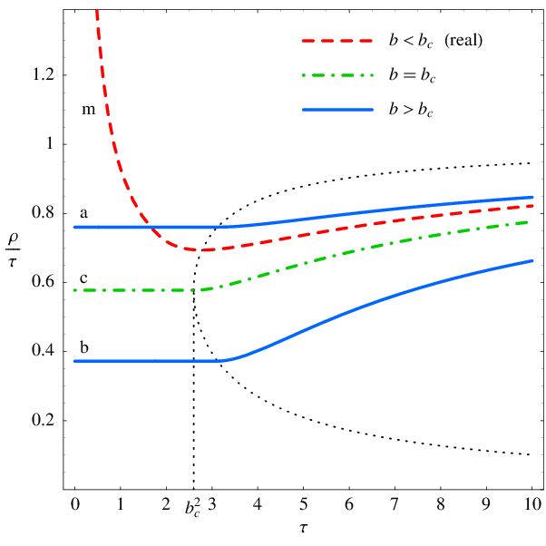

Due to the definition of , which has the kinematical factor , we see that such solutions show a singularity of the field of type , so that the metric coefficient must change sign at some value of and is singular at .
A clearcut interpretation of the (unphysical) real-valued solutions with and is not really available yet. However, we know that in about the same impact parameter region classical CTS do exist, as shown in [11, 12, 7]. It is therefore tempting to guess that such field configurations of the ACV approach (which are singular and should have negligible quantum weight) correspond to classically trapped surfaces. In this picture, the complex-valued solutions with (which are regular, and should have finite quantum weight) would correspond to the tunneling transition from the perturbative fields with and positive to the “untrapped” configuration with .
In order to develop the above suggestion, in the following we shall consider the action (11) at quantum level, by defining the -matrix as the path-integral over -field configurations induced by that action.
3 The quantum level and tunneling amplitude
The idea is to introduce the quantum -matrix as a path-integral in -space of the reduced-action exponential. In this “sum over actions” interpretation the semiclassical limit will automatically agree with the expression in eq. (11) above, which is based on the “on-shell” action. Furthermore, calculable quantum corrections will be introduced.
3.1 Quantized elastic -matrix
Following the above suggestion, and neglecting absorptive effects induced by the -field, we define
| (16) |
where we use the expression (11) of the reduced action, with the notation and we introduce the Lagrangian
| (17) |
with the boundary conditions introduced by ACV and discussed in sec. 2.
The definition (16) given above is equivalent, by a Legendre transform and use of the Trotter formula [14], to quantize the -evolution Hamiltonian to be introduced shortly, and to calculate the evolution operator , thus reducing the -matrix calculation to a known quantum quantum-mechanical problem. In fact, by eq. (17), we can introduce the “conjugate momentum”
| (18) |
and we obtain
| (19) |
from which the classical EOM (10) can be derived. Then, quantizing the evolution according to eq. (16) amounts to assume the canonical commutation relation
| (20) |
and to quantize the Hamiltonian (19) accordingly:
| (21) |
Finally, the path-integral (16) for the -matrix without absorption is related by Trotter’s formula to a tunneling amplitude involving the time-evolution operator :
| (22) |
where is calculated with -antiordering and the normalization of states will be fixed below.
We note that the commutation relation (20) does not follow from first principles, but is simply induced by the path-integral definition (16). Note also that here we allow fluctuations in transverse space, but we keep frozen the shock-wave dependence on the longitudinal variables . This means that our account of quantum fluctuations is admittedly incomplete and should be considered only as a first step towards the full quantum level. This step, defined by (16)-(22), has nevertheless the virtue of reproducing the semiclassical result for . Furthermore, we think that such commutation relations are of the expected order of magnitude. An argument in this direction is to notice that the shock-wave of ACV has wavefronts33 3 The second wavefront is better seen by replacing in eq. (1b) by , as argued in [1]. at and , and the latter implies at large negative times of order . Therefore, time- and -derivatives turn out to be related by a factor of as a consequence of a sort of retardation in the occurrence of that “precursor” wavefront, a factor which also occurs in the commutation relation (20). Finally, corrections of relative order are expected here, and at full quantum level also.
3.2 Inelastic -matrix and absorption
We have so far defined the -matrix as if no inelastic processes were present. However, the very existence of the emitted graviton field implies the existence of multi-graviton production and, by unitarity, of absorption in the elastic channel. Therefore, in order to find a unitary -matrix at quantum level, it is essential to introduce both phenomena. At semiclassical level, ACV noticed that the classical -field solution
| (23) |
induces in the eikonal formulation an inelastic -matrix which is approximately described by the coherent state operator
| (24) | ||||
| (25) |
where the operator incorporates both emission and absorption of the -fields and parametrizes the (-dependent) rapidity phase space which is effectively44 4 When energy conservation is taken into account [13], absorptive corrections consistent with the AGK cutting rules [15] suppress the fragmentation region in a -dependent way, so as to yield a purely central process for . allowed by energy conservation [13] . By normal ordering of (24), we derive the semiclassical elastic-channel absorption factor
| (26) |
which is dependent, of course, on the classical solution singled out at semiclassical level.
A possible way to extend the coherent state definition (24) to the quantum level, is just to introduce it in the path-integral formulation (16) as follows
| (27) |
where acts on the multi-graviton Fock space, but is to be considered as a c-number current with respect to the quantum variables .
In the elastic channel, the -dependent exponential in (27) is to be replaced by its vacuum expectation value . Of course, in this quantum extension of (26), no commitment is made to a particular classical solution so that the output will presumably contain a weighted superposition of the various classical paths satisfying the boundary conditions, that we shall calculate in the following.
3.3 Tunneling amplitude neglecting absorption
With the above warnings about the meaning of quantization and the role of inelasticity, let us derive a more detailed expression of the tunneling amplitude (22) without absorption
| (28) |
where the initial (final) state expresses the boundary condition (), is the time-dependent wave function, and is the evolution operator in the Schrödinger picture, calculated with -antiordering (according to the suggestion above that true time is related to ).
Since the Hamiltonian (19) is time-dependent, the expression of the wave function at time is related to the evolution due to the Coulomb Hamiltonian by
| (29) | ||||
| (30) |
where, according to eq. (21), we have used “free” evolution for . Therefore, the tunneling amplitude can be related to a Coulomb wave function as follows
| (31) |
where we note the free Gaussian propagator, acting on the continuum Coulomb wave function
| (32) |
The latter, due to the infinite evolution from the initial condition , is a solution of the stationary Coulomb problem
| (33) |
with zero energy eigenvalue (where from now on we express in units of ). The form of is better specified by the Lippman-Schwinger equation
| (34) |
and thus contains an incident wave with , plus a reflected wave for and a transmitted wave in the region.
We then conclude that the amplitude (22) is, by eq. (31), the convolution of a gaussian propagator with the Coulomb wave function , which has a tunneling interpretation with the Coulomb barrier. In fact, by eq. (34), it contains a transmitted wave in (where the Coulomb potential is attractive) and incident plus reflected waves in (where it is repulsive).
Note that, at we simply have , so that the tunneling interpretation is direct. On the other hand for , the convolution with the free propagator changes the problem considerably, and is the source of the critical impact parameter, as we shall see below.
4 Calculation of quantum tunneling amplitude
We shall now proceed to the actual calculation of the tunneling amplitude (31) without absorption in terms of the wave function (32). We shall then introduce absorption according to the definition (27), by discussing in particular the -matrix in the elastic channel.
4.1 The tunneling wave function and case
The explicit solution of (33) is given by a particular confluent hypergeometric function of defined as follows
| (35) |
where is defined in terms of its asymptotic power behaviour for and the normalization factor , to be found below, is chosen so as to have, asymptotically, a pure-phase incoming wave for , being an IR parameter used to factorize the Coulomb phase. We shall call this prescription as the “Coulomb phase” normalization at .
Here we note that the value in yields a degenerate case for the differential equation in (35) in which the standard solution with the outgoing wave, usually called [16], develops a singularity of the form . Then, the continuation to is determined by requiring the continuity of wave function and its flux at , as is appropriate for a principal part determination of the “Coulomb” singularity. The outcome involves therefore an important contribution at of the regular solution , so that we obtain
| (36) | ||||
We are finally able to determine the normalization factor and the value of , which is finite and non-vanishing, as follows
| (37) |
a value which is of order , the same order as the wave transmitted by the barrier.
In the case, the tunneling amplitude is simply the value in (37), with the normalization just discussed, and is of order , as our -matrix, leaving aside the coherent state describing multigraviton production. We obtain, from ACV and from eq. (37), a more detailed expression in terms of the known on-shell action (15), as follows
| (38) | ||||
We see that the tunneling amplitude provides the semiclassical result for the elastic -matrix and quantum corrections to it. It also determines, in a way to be discussed shortly, both normal graviton radiation and the corresponding absorption.
4.2 Integral representation of tunneling amplitude at
For , the calculation of in (31) involves a nontrivial integral, which should be investigated with care. A preliminary analysis can be performed in the WKB approximation, which is straightforward. In fact, by setting , we have
| (39) |
and the integral in (22) is dominated by a stationarity point at
| (40) |
yielding the phase
| (41) |
which reproduce both the criticality equation and the on-shell action of ACV, apart from an overall phase, which has not been determined in the expression (39).
The detailed calculation of , yielding quantum corrections also, is done by using standard Fourier-type representations for and [16] in eq. (36) and by performing the gaussian -integral in eq. (31). We then obtain the integral representation
| (42) |
where is a contour encircling the branch points at in the anticlockwise direction. In eq. (42), the limit is accounted for by the first term, while the second takes over for finite values, and is leading by a factor of for . The latter factor is exhibited by rewriting the contour integral in terms of the discontinuity of the integrand for .
More precisely, for sizeable values of , such that , eq. (42) is dominated by the second term which, by closing the contour on the branch-cut, takes the form
| (43) | ||||
| (44) |
where, as already noticed, the phase is closely related to the original action (15) when evaluated at the values satisfying the criticality condition.
It is interesting to note that the amplitude expression (42) resembles the “sum over solutions” interpretation of the -matrix in ACV, by setting and by choosing a proper measure factor. In fact, with this identification, the integrand carries the same phase as eq. (41) given before. Keep in mind, however, that the full semiclassical expression of the ACV -matrix carries also a coherent state factor yielding graviton radiation and the corresponding absorption of the elastic amplitude, given in terms of the field , for each value of . We think, therefore, that the expression (42) — valid as it stands for the “elastic” part of the action (11) — should be improved in order to extend it to inelastic processes and to take into account this effect.
4.3 Including absorption at quantum level
In order to take into account multi-graviton emission, the -matrix should be defined as in eq. (27). By limiting ourselves to the elastic channel, we should calculate the normal-ordering suppression factor analogous to (26), and we obtain
| (45) |
where the parameter effectively takes into account the longitudinal phase space, limited by energy conservation [13].
The absorption term in (45) adds an imaginary part to the kinetic term in the Lagrangian and formally changes the definition of the Hamiltonian and of the quantization condition in terms of a parameter
| (46) |
A simple way to take into account such changes is to solve the evolution equation for the wave-function directly in the momentum representation in which is diagonal. We simply obtain
| (47) |
where we have introduced the representation
| (48) |
For , the evolution involves the Coulomb-type Hamiltonian with zero energy (due to the boundary condition ) and we get the solution
| (49) |
where the normalization factor will be fixed later on. On the other hand, for we have just free evolution,
| (50) |
yielding
| (51) |
and therefore
| (52) |
Finally, by setting and we get the desired result, which differs from the representation (43) by an integration by parts, by a normalization factor and by the replacement .
We thus conclude that the elastic -matrix (or, the tunneling amplitude including absorption) is given by
| (53) |
where the factor is now computed by the “Coulomb phase” normalization condition on to be
| (54) |
4.4 Perturbative versus collapse-like regimes
The elastic -matrix resulting from eq. (53) improves the semiclassical approximation by providing a quantum weight to the various classical paths. Its modulus is plotted in fig. 2 for various values of and of the absorption parameter . Fig. 2a shows that the result oscillates, so that absorption (required for self-consistency because ) is essential to comply with elastic unitarity ().

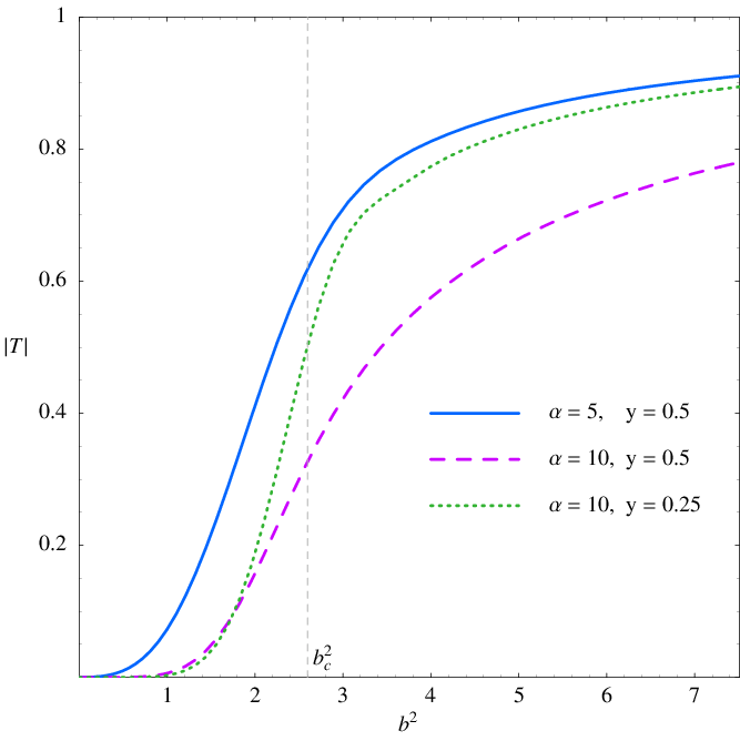
The oscillations appearing in fig. 2 in the limit are due to the fact that the quantum treatment embodies contributions from both the perturbative and the non-perturbative semiclassical solutions for . In the saddle point approximation one would have the simple formula
| (55) | ||||
If the absorption factor were neglected (as it happens in the limit), there would be strong interference of the two solutions, and large unitarity violations. For , on the other hand, the non-perturbative contribution is much more absorbed, and the result is dominated, for , by the perturbative contribution. This explains the overall agreement with the semiclassical result — also plotted in fig. 2a — with moderate quantum corrections. Finally, in fig. 2b we note the dependence of absorption on and . While for it is basically the product that matters, for absorption is dependent, but only weakly -dependent, showing a sort of universal behaviour up to sizeable values of .
The -matrix behaviour for requires a special discussion. When in eq. (55) approaches the critical value (or, ) at which the criticality equation is stationary, the two dominant contributions to (55) become of the same order, and the saddle points pinch and then become complex conjugate (at ). In such a situation the quadratic fluctuations diverge, and the quadratic expansion of the phase (44) has to be extended to the cubic terms, in order to stabilize the integration.
If absorption is included, this analysis has to be performed at complex values of , by assuming that is a small parameter (see app A). We expand the phase in (43) around the value such that , which is given precisely by eq. (14) and acquires the meaning of WKB turning point. To lowest order in we find the expression
| (56) |
which, replaced in eq. (53), yields the integral representation of an Airy function (cf. eq. (68)), by providing the approximate result
| (57) |
We see that the large- behaviour is characterized by the exponent for also. However, the modulus behaves differently for positive and negative ’s. Indeed, a simple evaluation yields
| (58) |
Therefore, the additional absorption with exponent for is unambiguously confirmed, and is continuously joined to the behaviour of normal absorption for . This provides a rise of the modulus in the small region, so as to match eventually the (small) perturbative absorption at large values of . Such features qualitatively explain the behaviour of absorption in the region, as pictured in fig. 2b, in particular the fact that, for , it is weakly -dependent.
The above analysis confirms the existence of a perturbative and a collapse-like regime, and also confirms the singularity of exponent for the asymptotic high-energy behaviour. However, we also see from eq. (57) that is not a real singularity of the -matrix, because the Airy function is an entire function of its argument . This means that the singularities due to the pinching solutions cancel each other at . The lack of a true singularity might favour the interpretation of the new regime as a collective phenomenon, rather than a signal of new states. However, since our quantization procedure is incomplete, it is not yet clear whether such a feature is kept at full quantum level, in the string-gravity framework.
5 Discussion
Here we have introduced a quantization procedure for the transverse-space dynamics of the ACV framework [1], which allows a deeper understanding of the transplanckian scattering matrix of light particles and of its high-energy regimes, by providing a quantum tunneling interpretation of the collapse-like regime .
Indeed, we have related the high-energy elastic -matrix to a tunneling amplitude in gravitational field space () from a weak-field configuration at large distances () to a regular field at short distances ( finite). The dynamics, embodied in the high-energy graviton emission vertex, provides an impact-parameter dependent Coulomb barrier in the “renormalized radius” . As a consequence, if the impact parameter is below some critical value , quantum tunneling is essential for the above configuration to occur and provides a calculable suppression of the elastic channel which corresponds to the complex semiclassical solutions of the ACV proposal [1].
The statement above summarizes the basic point that we meant to elucidate here. Furthermore, our quantum approach provides a deeper perspective on a number of other points.
- •
Introducing “normal” absorption (due to graviton emission) is essential for the -matrix to satisfy elastic unitarity, and in order to understand the relative weight of the various semiclassical solutions and, in particular, the dominance of the perturbative one for .
- •
Taking absorption into account amounts to consider a complex impact parameter , where parametrizes the rapidity phase space allowed by energy conservation [13] for graviton emission. This makes it possible to continue normal absorption below , thus matching the perturbative behaviour at large values to the “extra” tunneling suppression for . The latter is thus fully confirmed, and shows a sort of universality, in the sense that it is weakly -dependent.
- •
Quantum corrections are calculable, of relative order and tend to smooth out the semiclassical results. In particular, is a singularity of the asymptotic high-energy behaviour, but is not a singularity of the -matrix itself.
In the present paper we investigate the elastic -matrix only. Although absorptive effects are consistently taken into account and are essential to fulfill elastic unitarity, we do not consider inelastic matrix elements explicitly. Our quantum model can be extended, in principle, to inelastic channels according to eq. (27), by introducing some time-dependent external current which, however, makes the inelastic model no longer explicitly solvable. Furthermore, improvements are needed, for instance in connection with energy conservation [13]. For the above reasons a deeper analysis is desirable, and is deferred to further work. Hopefully, the outcome of such a work should be able to explain the mechanism by which inelastic unitarity can be satisfied.
Acknowledgements
We warmly thank Daniele Amati and Gabriele Veneziano for seminal discussions on the tunneling interpretation and Slava Rychkov for stimulating remarks on the role of multigraviton emission. Work supported in part by a PRIN grant (MIUR, Italy).
Appendix A Stationary-phase estimates of tunneling amplitude
In this appendix we provide analytic approximations for the tunneling amplitude (43) and the elastic scattering amplitude (53) when is a large parameter. This amounts to evaluate the -integral
| (59) |
in an approximate form, with given by eq. (44).
A.1 Quadratic expansion
Let us first look for stationary points of the phase given in eq. (44):
| (60) |
The stationary points are thus determined by the criticality condition (40), and for the integration interval contains two of the three real solutions:
| (61) | ||||||
| (62) |
The second derivative of the phase at the stationary points is given by
| (63) |
and increases with : , . Therefore, the fluctuations around the two saddle points are smaller and smaller at large , while the distance between them increases, allowing us to treat them separately for sufficiently large :
| (64) | ||||
| (65) |
The saddle-point estimate of the tunneling amplitude is therefore given by
| (66) |
where in the last equality we have used the Stirling approximation for valid when . The result (66) reproduces the elastic -matrix result eq. (55) without absorption ().
A.2 Cubic expansion
When the impact parameter approaches the critical value , the two gaussians centered at the saddle points overlap and cannot be considered separately. In particular, at the two saddle points coincide
| (67) |
and have infinite fluctuations, due to the vanishing of the second derivative . Therefore, an estimate of the integral (59) for requires an expansion of the phase up to the third order in . In order to exploit the Airy-function integral representation
| (68) |
we expand around the point where its second derivative vanishes:
| (69) |
while the third derivatives is given by
| (70) |
By denoting with the subscript the various quantities evaluated at , and by setting we obtain
| (71) |
In order to express the above results in terms of the impact parameter , it is convenient to introduce the (small) parameter such that
| (72) |
From eqs. (69,44,60,70) we have
| (73) |
and finally
| (74) |
The behaviour of the elastic scattering amplitude (53)
| (75) |
for and small can be obtained directly from eq. (74). In fact, if we denote
| (76) |
the complex parameter
| (77) |
is small. The factor is then given by the expression (74) with . The remaining factor can be rewritten as
| (78) |
and we obtain
| (79) |
from which we derive eq. (57). The r.h.s. of eq. (57) is obtained from the asymptotic behaviour
| (80) |
where we can consider the argument of to be large even for small , provided is large enough:
| (81) |
References
- [1] D. Amati, M. Ciafaloni and G. Veneziano, “Towards an -matrix Description of Gravitational Collapse,” JHEP 0802 (2008) 049 [arXiv:0712.1209 [hep-th]].
- [2] D. Amati, M. Ciafaloni and G. Veneziano, “Classical and quantum gravity effects from planckian energy superstring collisions,” Int. J. Mod. Phys. A 3 (1988) 1615.
- [3] D. Amati, M. Ciafaloni and G. Veneziano, “Effective action and all order gravitational eikonal at Planckian energies,” Nucl. Phys. B 403, 707 (1993).
- [4] L. N. Lipatov, “High-energy scattering in QCD and in quantum gravity and two-dimensional field theories,” Nucl. Phys. B 365 (1991) 614.
- [5] R. Kirschner and L. Szymanowski, “Effective action for high-energy scattering in gravity,” Phys. Rev. D 52 (1995) 2333 [arXiv:hep-th/9412087].
- [6] E. P. Verlinde and H. L. Verlinde, “High-energy scattering in quantum gravity,” Class. Quant. Grav. 10 (1993) S175.
- [7] G. Veneziano and J. Wosiek, “Exploring an -matrix for gravitational collapse,” arXiv:0804.3321 [hep-th]; “Exploring an -matrix for gravitational collapse II: a momentum space analysis,” arXiv:0805.2973 [hep-th].
- [8] G. Marchesini and E. Onofri, “High energy gravitational scattering: a numerical study,” arXiv:0803.0250 [hep-th].
- [9] L. N. Lipatov, “Multi-Regge processes in gravitation,” Sov. Phys. JETP 55 (1982) 582 [Zh. Eksp. Teor. Fiz. 82 (1982) 991].
- [10] M. Ademollo, A. Bellini and M. Ciafaloni, “Superstring Regge amplitudes and emission vertices,” Phys. Lett. B 223 (1989) 318.
- [11] D. M. Eardley and S. B. Giddings, “Classical black hole production in high-energy collisions,” Phys. Rev. D 66 (2002) 044011 [arXiv:gr-qc/0201034].
- [12] E. Kohlprath and G. Veneziano, “Black holes from high-energy beam-beam collisions,” JHEP 0206 (2002) 057 [arXiv:gr-qc/0203093].
- [13] M. Ciafaloni and G. Veneziano, in preparation.
- [14] see, e.g., M. Reed and B. Simon, “Methods of Modern Mathematical Physics,” Vol. 1 (New York, N. Y., 1972), p. 295.
- [15] V. A. Abramovsky, V. N. Gribov and O. V. Kancheli, “Character of inclusive spectra and fluctuations produced in inelastic processes by multi-pomeron exchange,” Yad. Fiz. 18 (1973) 595 [Sov. J. Nucl. Phys. 18 (1974) 308].
- [16] M. Abramowitz and I.A. Stegun, “Handbook of mathematical functions”, Dover publications.