Numerical study of the frustrated ferromagnetic spin- chain
Abstract
The ground state phase diagram of the frustrated ferromagnetic spin-1/2 chain is investigated using the exact diagonalization technique. It is shown that there is a jump in the spontaneous magnetization and the ground state of the system undergos to a phase transition from a ferromagnetic phase to a phase with dimer ordering between next-nearest-neighbor spins. Near the quantum transition point, the critical behavior of the ground state energy is analyzed numerically. Using a practical finite-size scaling approach, the critical exponent of the ground state energy is computed. Our numerical results are in good agreement with the results obtained by other theoretical approaches.
pacs
75.10.Jm, 75.10.PqI Introduction
The physics of frustrated quantum spin systems have been attracted much interest from experimental and theoretical points of view. The spin- Hamiltonian of the frustrated model on a periodic chain of -sites is
| (1) |
where represents the operator at the n-th site, and , are the nearest-neighbor (NN) and next-nearest-neighbor (NNN) interactions. We introduce the parameter for convenience.
This model with NN and NNN antiferromagnetic interactions () is well studied[1, 2, 3, 4, 5, 6, 7, 8]. This chain is well known to display a quantum phase transition from a gapless, translationally invariant state with algebraic spin correlations (the spin fluid phase) to dimer gapful state at [3]. At the Majumdar-Ghosh point[5], i.e. at , the ground state is exactly solvable. It is a doubly degenerate dimer product of singlet pairs on neighboring sites. In general, the ground state is doubly degenerate for . For large () an incommensurate phase appears in the ground state phase diagram[4, 6]. The behavior of frustrated chains in the presence of a uniform magnetic field was first studied by R. Chitra[9]. Recently the effect of a uniform magnetic field on the model has been discussed[10]. They have shown that a chiral phase emerges in isotropic frustrated spin chains as well, if they are subject to a strong external magnetic field. When and (AF-F), the system is believed to be in a gapless antiferromagnetic phase for any permissible values of and .
Relatively little attention has been paid to frustrated ferromagnetic chains, i.e., and . From experimental point of view, the recent discovery of materials are described by parameters with this combinations of signs. The is believed to be described[11, 12] by , and which lies in a different parameter regime with [13]. A recent study[14] of the thermodynamics of the model (1) was motivated by the experimental results for . From theoretical point of view, the later model has been subject of many studies[14, 15, 16, 17, 18, 19, 20]. The complete picture of the phases of this model as a function of the frustration parameter is unclear up to now.
In the case of and (F-AF) with , the ground state is fully ferromagnetic and lies in the subspace with the degeneracy , and becomes[15] an () incommensurate singlet state[21, 22] for , also the lattice translational symmetry is thought to be broken. It is suggested that in this incommensurate singlet state, the gap is strongly suppresed[23]. At the critical point , two distinct configurations with the energy
| (2) |
are the ground states[24]. One is fully ferromagnetic with , the other is a singlet state with . The wave function of the singlet state at is known exactly[24, 25].
In the vicinity of the critical point , at () the singlet ground state energy behaves as , where is a critical exponent. The classical approximation gives . The spin-wave theory as well as some other approximations[6, 17] do not change this critical exponent. In Ref.[26], using variational approaches, it has been shown that the quantum fluctuations definitely change the classical critical exponent. They conjectured that strong quantum fluctuations change the critical exponent and . In a recent work, Dmitriev et.al.[27] have studied the properties of this model using the perturbation theory (PT) in the small parameter characterizing the deviation from the transition point. They considered the Hamiltonian (1) as
| (3) |
with a small parameter . Since the perturbation conserves the total spin , the PT to the lowest singlet state of the Hamiltonian involves only singlet excited states. They showed that the PT allow them to estimate the critical exponent of the ground state energy as
| (4) |
which is in good agreement with their previous result[26]. On the other hand, they have claimed that the exact diagonalization of finite chains shows a complicated iregular size dependence of the ground state energy, which makes the numerical estimation of the critical exponent impossible[27]. In a very recent work, the ground state phase diagram of the spin-1/2 zigzag chain with weakly anisotropic ferromagnetic NN and antiferromagnetic NNN interactions is studied[28]. It is shown that the ground state phase diagram consists of the fully polarized ferromagnetic, the commensurate spin-liquid and the incommensurate phases.
In this paper, we present our numerical results on the ground state phase diagram of the 1D frustrated ferromagnetic spin-1/2 model. Our results are obtained using the exact diagonalization technique. In section 2, we present the results of exact diagonalization calculations on the ground state phase diagram of the model. In section 3, we discuss a practical finite-size scaling approach and find the critical exponent of the ground state energy in the vicinity of the critical point . Finally, the summary and conclusions are presented in section 4.
II The ground state phase diagram
An inportant goal in the study of quantum spin systems is the search for novel states emerging from competing interactions in the ground state phase diagram. In particular, the study of continuous phase transitions, has been one of the most fertile branches of theoretical physics in the last decades. Each phases can usually be characterized by an order parameter. Often, the choice of an order parameter is obvious, however in some cases finding an appropriate order parameter is complicated. As we mensioned, the complete picture of the phases of this model as a function of the frustration parameter is not completely clear. It is known that the ground state is ferromagnetic at and a second order phase transition happens to the incommensurate singlet phase.

In order to explore the nature of the spectrum and the phase transition, we used the Lanczos method to diagonalize numerically finite (up to sites) chain systems. The energies of the few lowest eigenstates were obtained for chains with periodic boundary conditions. The Lanczos method and the related recursion methods,[30, 31, 32, 33] possibly with appropriate implementations, have emerged as one of the most important computational procedures, mainly when a few extreme eigenvalues are desired.
To recognize the different phases induced by the NNN exchange interaction in the ground state phase diagram, we have implemented the Lanczos algorithm of finite size chains to calculate the order parameters and the various spin correlation functions. The first insight into the nature of the different phases can be obtained by studying the uniform magnetization
| (5) |
where the notation represent the expectation value at the lowest energy state.
In Fig. 1 we have plotted the spontaneous magnetization, vs for the chain of different lengths . For arriving at this plot we considered and different values of the parameter . One of the most interesting known properties of this model is that the magnetization as a function of applied magnetic field displays a jump for certain parameters[34, 35, 18]. It can be seen that the spontaneous magnetization , remains close to the saturation value for . This behavior is in agreement with expectations based on the general statement that for values of the parameter , the ground state is in the gapped ferromagnetic phase. At a critical value , the spontaneous magnetization jumps to zero. However, we observe that the metamagnetic phase transition occurs also in the absence of the external uniform magnetic field. The zero value of the spontaneous magnetization in the region , shows that the ground state of the model is not magnetic.


To disply the ground state magnetic phase dagram of the model we have calculated the dimer order parameters. Because of two type of coupling constants, we introduce two kind of dimerization as
| (6) |
| (7) |
It is clear that the parameter is the F(AF)-dimer order parameter. In Fig. 2a(b) we have plotted F(AF)-dimer order parameter as a function of the parameter for the chain with and different values of the chain lengths . As is clearly seen from this figure, for , and are very close to , which confirm that the ground state of the system is in the fully polarized ferromagnetic phase. For and enough large values of parameter , F-dimer order parameter is slightly more than zero but the AF-dimer order parameter is less than saturation value () . Thus, increasing the antiferromagnetic exchang from critical value , quantum fluctuations suppress the ferromagnetic ordering and the system smoothly undergoes a transition from a ferromagnetic phase into a phase with the dimer ordering between the NNN spins. In this case of finite systems and with chosen values of the exchanges, due to the quantum fluctuations the values of the order parameters and deviate from the classical values in the region . The oscilations of and (quasi-plateau’s) at finite in the region , are the result of level crossing between the ground state and excited states of the model.
To obtain additional insight into the nature of different phases, we have also calculated the and components of the dimer-order parameters. We have found that is very close to the saturation value in the region . The dimerization perpendicular to the axis remains small and close to zero in complete agreement with the magnetization results. As soon as the antiferromagnetic exchange increases from the critical value , jumps to zero. However, all components of the F-dimer order parameter () remain close to zero in the region . Which shows that there is no long-range ferromagnetic order in the region . In contrast, components of the AF-dimer order parameter () smothly change from almost zero to the value . Due to the quantum fluctuations induced by the ferromagnetic exchange , the value of these components deviate from the saturation value .
Thus, our numerical results show that the ground state phase diagram of the frustrated ferromagnetic spin- chain for small values of the antiferromagnetic exchange () contains, besides the gapped ferromagnetic phase, the AF-dimer phase. Each phase is characterized by its own type of long-range order: the ferromagnetic order along axis in the ferromagnetic phase; the AF-dimer order between NNN spins in the AF-dimer phase.
III the scaling behavior of the ground state energy
The finite size scaling method is a way of extracting values for critical exponents by observing how measured quantities vary as the size (a is the lattice spacing and we will consider to be one) of the system studied changes. In fact, this method consists of comparing a sequence of finite lattices. The finite lattice systems are solved exactly, and various quantities can be calculated as a function of the lattice size , for small . Finally, these functions are scaled up to [29]. Two steps are needed before these ideas can be realized. First, one needs a procedure for solving the finite lattice systems exactly. Second, one needs a procedure for extrapolating from finite to infinite . In the step one, we have used the Lanczos method to obtain the ground state energy. We also checked our numerical results by the modified Lanczos method[36]. Using the modified Lanczos method one can get the excited state energies at the same accuracy as the ground state one. We did not find any irregular size dependence of the ground state energy in our numerical results. In the following, we present our finite-size scaling approach for the ground state energy.
Using Lanczos method, we can compute the ground state energy as a function of the chain length and the parameter as . We have implemented the modified Lanczos algorithm on finite size chains () by using periodic boundary conditions to calculate the ground state energy as a function of the parameter .
In the case of , the spectrum of the 1D F-AF model is gapless. The ground state energy in the thermodynamic limit behaves as Eq.(2). By checking the behavior of the function as a function of (), found the best fit to our data yielded and , which shows very good agreement with the analytical result Eq.(2).
Now let us introduce our finite size scaling procedure to find the correct critical exponent of the ground state energy in the vicinity of the critical point . First, we write the scaling function as the following expression,
| (8) |
where is a scaling parameter. As expected, the behavior of this equation in the combined limit
| (9) |
is consistent with Eq.(4). Thus it can be assumed that the asymptotic form of the scaling function is
| (10) |
and the -exponent in the large- regime () must be equal to one (). Then we get in the large- regime
| (11) |
This equation shows that the large- behavior of the scaling function is linear in where the scaling exponent of the ground state energy is . We should note that in using the Lanczos method we are limited to consider the maximum value of [37]. Moreover, since the scaling behavior is restricted to the limit , we should consider as soos as possible very small values of . Therefore, the value of cannot be increased in this method. However, we are not allowed to read the scaling exponent of the ground state energy which exists in the thermodynamic limit ( or ). Thus, we have to find the scaling behavior from the small- regime. According to our numerical computations where , the small- regime is equivalent to very small values of the parameter . In this case the ground state energy of the finite size system basically represents the perturbative behavior[37]
| (12) | |||||
The effect of higher-order terms can be neglected for to a very good approximation. The first coefficient in the perturbation expansion is the same as .

To find a relation between other coefficients and correct critical exponent of the ground state energy, it is more convenient rewrite Eq.(8) as[38]
| (13) |
where . This implies
| (14) |
where is the order of the leading term in the perturbation expansion. Using Eq.(12) we obtain
| (15) |
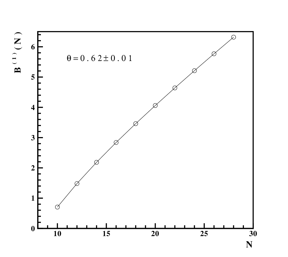
Now, if we consider the large- behavior of as
| (16) |
we find that the critical exponent of the ground state energy is related to the -exponent as,
| (17) |
The above arguments suggest that we should look for the large- behavior of the coefficient . To do this, in the first step we plotted in Fig. 3 the ground state energy versus for a fixed size . The best fit to our data is obtained with (), which shows that the first nonzero correction in the perturbation expansion is the first-order (). We have also implemented our procedure for different values of the sizes and found the same results for as we expected.
In the second step, we fitted the results of the ground state energy to the polynomials for close to as Eq.(12) up to . Using this procedure we found the coefficient of the first-order correction perturbation, , as a function of . Then we plotted in Fig. 4 the function versus . The results have been plotted for different sizes to derive the -exponent defined in Eq.(16). We found the best fit data for . Therefore, using Eq.(17) we have computed the ground state energy exponent . Our numerical results show very good agreement with the exponent derived in the theoretical point of view, Eq.(4).
IV summary
To summarize, we have studied the ground state phase diagram of the frustrated ferromagnetic spin-1/2 chain for small values of parameter . We have implemented the Lanczos method to obtain the ground state energy in small chains. The modified Lanczos method[32] is used also for checking the numerical results. Using the exact diagonalization results, we have calculated the various order parameters and spin structure factors as a function of the parameter . It is found that the spontaneous magnetization jumps to zero at the critical value . Increasing the antiferromagnetic exchange from critical value , the system smoothly undergoes a transition from a ferromagnetic phase into a phase with the dimer ordering between the NNN spins.
On the other hand, it is believed that the ground state energy behaves as , where is a critical exponent. From the classical approximations and the spin-wave theory, it had been obtained . Using the variational approaches and perturbation theory, it had been shown that the quantum fluctuations definitely change the critical exponent and . On the other hand, it had been believed that the exact diagonalization of finite chains shows a complicated iregular size dependence of the ground state energy, which makes the numerical estimation of the critical exponent impossible[27].
In this paper, we have used the finite-size scaling approach to investigate the critical exponent of the ground state energy. To estimate the critical exponent of the ground state energy, we have introduced a proper scaling function as Eq.(8). The scaling variable is defined as . According to our approach the right scaling exponent of the ground state energy gives a linear behavior of the scaling function versus for large . But, the Lanczos numerical results are not able to get the large- behavior.
To find the correct critical exponent of the ground state energy in the small- regime (), we have plotted the best fit to the data of the scaling function , which is the coefficient of the -order perturbation expansion of the ground state energy. The critical exponent of the ground state energy is computed with the relation between the divergence of the leading term () in the perturbation expansion and the scaling behavior of the ground state energy (Eq.(17)). Our numerical results, confirm that the quantum fluctuations are very important and change the critical exponent from the classical value and , in good agreement with the analytical results(Eq.(4)).
V Acknowledgments
I would like to thank G. I. Japaridze and T. Vekua for insightful comments and fruitful discussions that led to an improvement of this work.
References
References
- [1] F. D. Haldane, Phys. Rev. B 25, R4925 (1982).
- [2] T. Tonegawa and I. Harada, J. Phys. Soc. Jpn. 56, 2153 (1987).
- [3] K. Nomura and K. Okamoto, Phys. Lett. A 169, 433 (1992).
- [4] R. Bursill, G. A. Gehring, D. J. J. Farnell, J. B. Parkinson, T. Xiang, and C. Zeng, J. Phys: Condens. Matter 7, 8605 (1995).
- [5] C. K. Majumdar and D. K. Ghosh, J. Math. Phys. 10, 1388 (1969).
- [6] S. R. White and I. Affleck, Phys. Rev. B 54, 9862 (1996).
- [7] G. Bouzerar, A. P. Kampf, and G. I. Japaridze, Phys. Rev. B 58, 3117 (1998).
- [8] R. Jafari, and A. Langari, Physica A 364, 213 (2006).
- [9] R. Chitra, and T. Giamarchi, Phys. Rev. B 55, 5816 (1997).
- [10] A. Kolezuk and T. Vekua, Phys. Rev. B 72, 094424 (2005).
- [11] S. -L. Drechsler, et.al. J. Phys: Condens. Matter 18, 1 (2006).
- [12] M. Hase, H. Kuroe, K. Ozawa, O. Suzuki, H. Kitazawa, G. Kido, and T. Sekine, Phys. Rev. B 70, 104426 (2004).
- [13] M. Enderle, et.al. Europhys. Lett. 70, 237 (2005).
- [14] F. Heidrich-Meisner, A. Honecker, and T. Vekua, Phys. Rev. B 74, R020403 (2006).
- [15] T. Tonegawa and I. Harada, J. Phys. Soc. Jpn. 58, 2902 (1989).
- [16] A. V. Chubukov, Phys. Rev. B 44, R4693 (1991).
- [17] V. Ya. Krivnov and A. A. Ovchinikov, Phys. Rev. B 53, 6435 (1996).
- [18] A. A. Aligia, Phys. Rev. B 63, 014402 (2001).
- [19] H. T. Lu, Y. J. Wang, S. Qin, and T. Xiang, Phys. Rev. B 74, 134425 (2006).
- [20] R. Jafari, and A. Langari, Phys. Rev. B 76, 014412 (2007).
- [21] H. P. Bader and R. Schilling, Phys. Rev. B 19, 3556 (1979).
- [22] T. Hamada, J. Kane, S. Nakagawa and Y. Natsume, J. Phys. Soc. Jpn. 57, 1891 (1988); 58, 3869 (1989)
- [23] C. Itoi and S. Qin, Phys. Rev. B 63, 224423 (2001).
- [24] T. Hamada, J. Kane, S. Nakagawa, and Y. Natsume, J. Phys. Soc. Jpn. 57, 1891 (1988).
- [25] D. Dmitriev, V. Ya. Krivnov, and A. A. Ovchinikov, Phys. Rev. B 56, 5985 (1997).
- [26] D. Dmitriev and V. Ya. Krivnov, Phys. Rev. B 73, 024402 (2006).
- [27] D. Dmitriev and V. Ya. Krivnov, and J. Richter, Phys. Rev. B 75, 014424 (2007).
- [28] D. Dmitriev and V. Ya. Krivnov, Phys. Rev. B 77, 024401 (2008).
- [29] K. Okamoto,H. Nishimori, and Y. Taguchi, J. Phys. Soc. Jpn. 55, 1458 (1986).
- [30] C. Lanczos, J. Res. Natl. Bur. Stand. 45, 255 (1950).
- [31] R. Haydock, V. Heine, and M. J. Kelly, J. Phys. C 5, 2845 (1972); 8, 2591 (1975).
- [32] G. Grosso and G. Pastori Parravicini, Adv. Chem. Phys. 62, 81133 (1985).
- [33] H. Q. Lin and J. E. Gubernatis, Comput. Phys. 7, 400 (1993).
- [34] C. Gerhardt, K. -H. Mutter and H. Kroger, Phys. Rev. B 57, 11504 (1998).
- [35] S. Hirata, cond-mat/9912066.
- [36] G. Grosso and L. Martinelli, Phys. Rev. B 51, 13033 (1995).
- [37] A. Langari and S. Mahdavifar, Phys. Rev. B 73, 1 (2006).
- [38] H. R. Roomany, H. W. Wyld, and L. E. Holloway, Phys. Rev. D 21, 6 (1980).