ENTANGLEMENT-ASSISTED CODING THEORY.

Min-Hsiu Hsieh

August 2008

Chapter 1: Overview

The theory of quantum mechanics, founded in the early 1920s, ended the turmoil caused by the classical physics that predicted various absurd results such as electrons spiraling inexorably into the atom nucleus. Though the mathematical framework of quantum mechanics is simple, even geniuses like Albert Einstein found it counter-intuitive. Generations of physicists since put a lot of effort to sharpen our intuition about quantum mechanics, and make it more transparent to normal human minds. Several fundamental results discovered later on, such as the famous no-cloning theorem [58] that denies the possibility of using quantum effects to signal faster than light, help us better understand quantum mechanics.

Research on quantum mechanics evolved into a interdisciplinary science due to several successful applications of quantum effects on classical computation and communication problems in 1990s. Among them, Shor proposed a quantum algorithm for the enormously important problem [53] — the problem of finding the prime factors of an integer — showing exponential speed-up over the best known classical algorithm. This result not only attracted broad interest because this problem is believed to have no efficient solution on classical computers, but also provided strong evidence that quantum computers are more powerful than classical computers.

However, the power of quantum computation and communication over classical computation and communication comes from implementing entangled quantum states that are easily spoilt by their vulnerability to errors. Namely, the destructive interference of the omnipresent environment leads to an exponential loss of the probability that the computation runs in the desired way. Up to that point, there was a widespread belief that decoherence — environmental noise — would doom any chance of building large scale quantum computers or quantum communication protocols. The equally widespread belief that any analogue of classical error correction was impossible in quantum mechanics due to the famous no cloning theorem produced an even stronger pessimistic atmosphere in developing quantum computers.

Luckily, the pessimistic atmosphere did not last long. One of the most important discoveries in quantum information science, the existence of quantum error-correcting codes (QECCs), defied those expectations. The first quantum error-correcting code, considered as a quantum analogue of the classical repetition code, was proposed by Shor in 1995 [52]. The theory of quantum error correction quickly became a popular research topic. The quantum error-correcting conditions were proved independently by Bennett, DiVincenzo, Smolin and Wootters [5], and by Knill and Laflamme [34]. The best quantum code that encodes one-qubit information, the five-qubit code, was discovered by Laflamme, Miquel, Paz, and Zurek [39], and independently by [5].

The development of quantum error-correcting theory then became systematic. A construction of Calderbank, Shor, and Steane [16, 55] showed that it was possible to construct quantum codes from classical linear codes — the CSS codes — thereby drawing on the well-studied theory of classical error correction. Furthermore, Gottesman invented the stabilizer formalism [28], and used it to define stabilizer codes. In this view, quantum error-correcting codes are simultaneous eigenspaces of a group of commuting operators, the stabilizer. Independently, Calderbank, Rain, Shor, and Sloane [14] proposed a similar idea to define quantum codes based on orthogonal geometry in classical coding theory. This result connected quantum codes to classical quaternary codes [15]. The theory of quantum error correction developed so far is called standard quantum error correction.

Important as these results were, they fell short of doing everything that one might wish. The connection between classical codes and quantum codes was not universal. Rather, only classical codes which satisfied a self-orthogonality constraint could be used to construct quantum codes. While this constraint was not too difficult to satisfy for relatively small codes, it is a substantial barrier to the use of highly efficient modern codes, such as Turbo and Low-Density Parity Check (LDPC) codes, in quantum information theory. These codes are capable of achieving the classical capacity; but the difficulty of constructing self-orthogonal versions of them has made progress toward finding quantum versions very slow.

These problems can be overcome with pre-existing entanglement. Entanglement plays a central role in almost every quantum computation and communication task. It enables the teleportation of quantum states without physically sending quantum systems[4]; it doubles the capacity of quantum channels for sending classical information[6]; it is known to be necessary for the power of quantum computation[8, 31]. Furthermore, descriptions in quantum information theory are often simplified by the assumption that pre-existing entanglement is available.

In the thesis, we show how shared entanglement provides a simpler and more fundamental theory of quantum error correction, and at the same time greatly generalize the existing theory of quantum error correction. If the CSS construction for quantum codes is applied to a classical code which is not self-orthogonal, the resulting “stabilizer” group is not commuting, and thus has no code space. We are able to avoid this problem by making use of pre-existing entanglement. This noncommuting stabilizer group can be embedded in a larger space, which makes the group commute, and allows a code space to be defined. Moreover, this construction can be applied to any classical quaternary code, not just self-orthogonal ones. The existing theory of quantum error-correcting codes thus becomes a special case of our theory: self-orthogonal classical codes give rise to standard quantum codes, while non-self-orthogonal classical codes give rise to entanglement-assisted codes.

Besides the entanglement-assisted formalism [13, 12] we proposed in this thesis, there has been one other major breakthrough in quantum error correction theory: the discovery of operator quantum error-correcting codes (OQECCs) [1, 2, 3, 33, 37, 38, 48, 50], or subsystem codes. Instead of encoding quantum information into a subspace, OQECCs encode quantum information into a subsystem of the subspace. These provide a general theory which combines passive error-avoiding schemes, such as decoherence-free subspaces [61, 40] and noiseless subsystems [35, 32, 59, 60], with conventional (active) quantum error correction. OQECCs do not lead to new codes, but instead provide a new kind of decoding procedure: it is not necessary to actively correct all errors, but rather only to perform correction modulo the subsystem structure. One potential benefit of the new decoding procedure is to improve the threshold of fault-tolerant quantum computation [2].

The other major contribution of this thesis is the development of the unifying formalism that unifies these two extensions of standard QECCs: the operator quantum error-correcting codes (OQECCs), and the entanglement-assisted quantum error-correcting codes (EAQECCs). Furthermore, our formalism retains the advantages of both entanglement-assisted and operator quantum error correction. On one hand, OQECCs provide a general theory which combines passive error-avoiding schemes with standard quantum error correction. On the other hand, EAQECCs provide a general theory which links any classical quaternary code, not just self-orthogonal ones, to a quantum code. In addition to presenting our formal theory, we have given several examples of code construction. These examples demonstrate that our formalism can be used to construct quantum codes tailored to the needs of particular applications.

Because classical LDPC codes have such high performance — approaching the channel capacity in the limit of large block size — there has been considerable interest in finding quantum versions of these codes. However, quantum low-density parity-check codes [30, 44, 17, 20] are far less studied than their classical counterparts. The main obstacle comes from the dual-containing constraint of the classical codes that are used to construct the corresponding quantum codes. The second obstacle comes from the bad performance of the iterative decoding algorithm such as the famous sum-product algorithm (SPA). Though the SPA decoding can be directly used to decode the quantum errors, its performance is severely limited by the many 4-cycles, which are usually the by-product of the dual-containing property, in the standard quantum LDPC codes [44].

In the last part of the thesis, we will show that, with the entanglement-assisted formalism [13, 12], these two obstacles of standard quantum LDPC codes can be overcome. By allowing the use of pre-shared entanglement between senders and receivers, the dual-containing constraint can be removed. Constructing quantum LDPC codes from classical LDPC codes becomes transparent. That is, arbitrary classical quaternary codes can be used to construct quantum codes via the generalized CSS construction [13]. Furthermore, we can easily construct quantum LDPC codes from classical LDPC codes with girth at least 6. We make use of classical quasi-cyclic LDPC codes in our construction, and show that given similar net yield these quantum LDPC codes perform better than the standard quantum LDPC codes by numerical simulation.

This thesis is organized as follows. We give various background materials in chapter 2. In chapter 3, we introduce standard QECCs using the canonical code method and stabilizer formalism. In chapter 4, we present our first result: the entanglement-assisted formalism. In chapter 5, we introduce operator quantum error-correcting codes. In chapter 6, we present our second result: the entanglement-assisted operator formalism. Finally, we show how to use the entanglement-assisted formalism to construct quantum LDPC codes with better performance in chapter 7. Notice that we explicitly assume a communication scenario throughout the thesis. That is, noise is modeled as a quantum channel, and it only happens in the channel. Two parties involved in the information processing are called sender and receiver, respectively, and their operations on the quantum states are assumed to be noise-free.

Chapter 2: Background knowledge

2.1 Single qubit Pauli group

The set of Pauli matrices over a two-dimensional Hilbert space ${\cal H}_{2}$ is defined as

I=\left[\begin{array}[]{cc}1&0\\ 0&1\end{array}\right],\quad X=\left[\begin{array}[]{cc}0&1\\ 1&0\end{array}\right],\quad

Y=\left[\begin{array}[]{cc}0&-i\\ i&0\end{array}\right],\quad Z=\left[\begin{array}[]{cc}1&0\\ 0&-1\end{array}\right].

The Pauli matrices are Hermitian unitary matrices with eigenvalues belonging to the set $\{1,-1\}$ . The multiplication table of these matrices is given by:

\begin{array}[]{|c|cccc|}\hline\cr\times&I&X&Y&Z\\ \hline\cr I&I&X&Y&Z\\ X&X&I&iZ&-iY\\ Y&Y&-iZ&I&iX\\ Z&Z&iY&-iX&I\\ \hline\cr\end{array}

Observe that the Pauli matrices either commute or anticommute. Let $[S]=\{\beta S\mid\beta\in\mathbb{C},|\beta|=1\}$ be the equivalence class of matrices equal to $S$ up to a phase factor.^*^* * It makes good physical sense to neglect this overall phase, which has no observable consequence. Let ${\cal G}$ be the group generated by the set of Pauli matrices $\{I,X,Y,Z\}$ with all possible phases, then the set $[{\cal G}]=\{[I],[X],[Y],[Z]\}$ is readily seen to form a commutative group under the multiplication operation defined by $[S][T]=[ST]$ . We called $[{\cal G}]$ the Pauli group.

We are interested in relating the Pauli group to the additive group $(\mathbb{Z}_{2})^{2}=\{00,01,10,11\}$ of binary words of length $2$ described by the table:

\begin{array}[]{|c|cccc|}\hline\cr+&00&01&11&10\\ \hline\cr 00&00&01&11&10\\ 01&01&00&10&11\\ 11&11&10&00&01\\ 10&10&11&01&00\\ \hline\cr\end{array}

This group is also a two-dimensional vector space over the field $\mathbb{Z}_{2}$ . A bilinear form can be defined over this vector space, called the symplectic form or symplectic product^†^† † Strictly speaking it is not an inner product. $\odot:(\mathbb{Z}_{2})^{2}\times(\mathbb{Z}_{2})^{2}\rightarrow\mathbb{Z}_{2}$ , given by the table

\begin{array}[]{|c|cccc|}\hline\cr\odot&00&01&11&10\\ \hline\cr 00&0&0&0&0\\ 01&0&0&1&1\\ 11&0&1&0&1\\ 10&0&1&1&0\\ \hline\cr\end{array}

In what follows we will often write elements of $(\mathbb{Z}_{2})^{2}$ as $u=(z|x)$ , with $z,x\in\mathbb{Z}_{2}$ . For instance, $01$ becomes $(0|1)$ . For $u=(z|x),v=(z^{\prime}|x^{\prime})\in(\mathbb{Z}_{2})^{2}$ the symplectic product is equivalently defined by

u\odot v=zx^{\prime}+z^{\prime}x.

Define the map $N:(\mathbb{Z}_{2})^{2}\to{\cal G}$ by the following table:

\begin{array}[]{|c|c|}\hline\cr(\mathbb{Z}_{2})^{2}&{\cal G}\\ \hline\cr 00&I\\ 01&X\\ 11&Y\\ 10&Z\\ \hline\cr\end{array}

This map is defined in such a way that $N_{(z|x)}$ and $Z^{z}X^{x}$ are equal up to a phase factor, i.e.

[N_{(z|x)}]=[Z^{z}X^{x}].

We make two key observations

(1).

The map $[N]:(\mathbb{Z}_{2})^{2}\to[{\cal G}]$ induced by $N$ is an isomorphism:

$[N_{u}][N_{v}]=[N_{u+v}].$
(2).

The commutation relations of the Pauli matrices are captured by the symplectic product

$N_{u}N_{v}=(-1)^{u\odot v}N_{v}N_{u}.$

Both properties are readily verified from the tables.

2.2 Multi-qubit Pauli group

Consider an $n$ -qubit system corresponding to the tensor product Hilbert space ${\cal H}_{2}^{\otimes n}$ . Define an $n$ -qubit Pauli matrix ${\mathbf{S}}$ to be of the form ${\mathbf{S}}=S_{1}\otimes S_{2}\otimes\cdots\otimes S_{n}$ , where $S_{j}\in{\cal G}$ . Let ${\cal G}^{n}$ be the group of all $4^{n}$ $n$ -qubit Pauli matrices with all possible phases. Define as before the equivalence class $[{\mathbf{S}}]=\{\beta{\mathbf{S}}\mid\beta\in\mathbb{C},|\beta|=1\}$ . Then

[{\mathbf{S}}][{\mathbf{T}}]=[S_{1}T_{1}]\otimes[S_{2}T_{2}]\otimes\cdots\otimes[S_{n}T_{n}]=[{\mathbf{S}}{\mathbf{T}}].

Thus the set $[{\cal G}^{n}]=\{[{\mathbf{S}}]:{\mathbf{S}}\in{\cal G}^{n}\}$ is a commutative multiplicative group, and is called the $n$ -fold Pauli Group.

Now consider the group/vector space $(\mathbb{Z}_{2})^{2n}$ of binary vectors of length $2n$ . Its elements may be written as ${\mathbf{u}}=({\mathbf{z}}|{\mathbf{x}})$ , ${\mathbf{z}}=z_{1}\dots z_{n}\in(\mathbb{Z}_{2})^{n}$ , ${\mathbf{x}}=x_{1}\dots x_{n}\in(\mathbb{Z}_{2})^{n}$ . We shall think of ${\mathbf{u}}$ , ${\mathbf{z}}$ and ${\mathbf{x}}$ as row vectors. The symplectic product of ${\mathbf{u}}=({\mathbf{z}}|{\mathbf{x}})$ and ${\mathbf{v}}=({\mathbf{z}}^{\prime}|{\mathbf{x}}^{\prime})$ is given by

{\mathbf{u}}\odot{\mathbf{v}}^{{{T}}}={\mathbf{z}}\,{{\mathbf{x}}^{\prime}}^{{{T}}}+{\mathbf{z}}^{\prime}\,{\mathbf{x}}^{{{T}}}.

The right hand side are binary inner products and the superscript ${{T}}$ denotes the transpose. This should be thought of as a kind of matrix multiplication of a row vector and a column vector. We use ${\mathbf{u}}\odot{\mathbf{v}}^{{{T}}}$ rather than the more standard ${\mathbf{u}}\,{\mathbf{v}}^{{T}}$ to emphasize that the symplectic form is used rather than the binary inner product. Equivalently,

{\mathbf{u}}\odot{\mathbf{v}}^{{T}}=\sum_{i}u_{i}\odot v_{i}

where $u_{i}=(z_{i}|x_{i}),v_{i}=(z^{\prime}_{i}|x^{\prime}_{i})$ and this sum represents Boolean addition. Observe that if ${{\mathbf{u}}}\odot{{\mathbf{v}}}^{{T}}=0$ , these two vectors are “orthogonal” to each other with respect to the symplectic inner product.

The map $N:(\mathbb{Z}_{2})^{2n}\rightarrow{\cal G}^{n}$ is now defined as

N_{\mathbf{u}}=N_{u_{1}}\otimes\dots\otimes N_{u_{n}}.

Writing

X^{{\mathbf{x}}}=X^{x_{1}}\otimes\dots\otimes X^{x_{n}},

Z^{{\mathbf{z}}}=Z^{z_{1}}\otimes\dots\otimes Z^{z_{n}},

as in the single qubit case, we have

[N_{({\mathbf{z}}|{\mathbf{x}})}]=[Z^{{\mathbf{z}}}X^{{\mathbf{x}}}].

The two observations made for the single qubit case also hold:

(1).

The map $[N]:(\mathbb{Z}_{2})^{2n}\to[{\cal G}^{n}]$ induced by $N$ is an isomorphism:

$[N_{\mathbf{u}}][N_{\mathbf{v}}]=[N_{{\mathbf{u}}+{\mathbf{v}}}].$ (1)

Consequently, if $\{{\mathbf{u}}_{1},\dots,{\mathbf{u}}_{m}\}$ is a linearly independent set then the elements of the Pauli group subset $\{[N_{{\mathbf{u}}_{1}}],\dots,[N_{{\mathbf{u}}_{m}}]\}$ are independent in the sense that no element can be written as a product of others.
(2).

The commutation relations of the $n$ -qubit Pauli matrices are captured by the symplectic product

$N_{\mathbf{u}}N_{\mathbf{v}}=(-1)^{{\mathbf{u}}\odot{\mathbf{v}}^{{T}}}N_{\mathbf{v}}N_{\mathbf{u}}.$ (2)

We define the weight of a Pauli operator $N_{\mathbf{u}}$ , $\wt(N_{\mathbf{u}})$ , to be the number of single-qubit Pauli matrices in $N_{\mathbf{u}}$ not equal to the identity $I$ . Define the weight of a vector ${\mathbf{u}}=({\mathbf{z}}|{\mathbf{x}})\in(\mathbb{Z}_{2})^{2n}$ by $\wt_{\rm sp}({\mathbf{u}})=\wt_{2}({\mathbf{z}}\vee{\mathbf{x}})$ . Here $\vee$ denotes the bitwise logical “or”, and $\wt_{2}({\mathbf{y}})$ is the number of non-zero bits in ${\mathbf{y}}\in(\mathbb{Z}_{2})^{n}$ . It is easy to verify that

\wt(N_{{\mathbf{u}}})=\wt_{\rm sp}({\mathbf{u}}).

2.3 Properties of the symplectic form

A subspace $V$ of $(\mathbb{Z}_{2})^{2n}$ is called symplectic [18] if there is no ${\mathbf{v}}\in V$ such that

{\mathbf{v}}\odot{\mathbf{u}}^{{T}}=0,\,\,\,\forall{\mathbf{u}}\in V.

(3)

$(\mathbb{Z}_{2})^{2n}$ is itself a symplectic subspace. Consider the standard basis for $(\mathbb{Z}_{2})^{2n}$ , consisting of ${\mathbf{g}}_{i}=({\mathbf{e}}_{i}|\mathbf{0})$ and ${\mathbf{h}}_{i}=(\mathbf{0}|{\mathbf{e}}_{i})$ for $i=1,\dots,n$ , where ${\mathbf{e}}_{i}=(0,\dots,0,1,0,\dots,0)$ [ $1$ in the $i$ th position] are the standard basis vectors of $(\mathbb{Z}_{2})^{n}$ . Observe that

$\displaystyle{\mathbf{g}}_{i}\odot{\mathbf{g}}_{j}^{{T}}=0,$	$\displaystyle{\rm for\,\,all\,\,}i,j$	(4)
$\displaystyle{\mathbf{h}}_{i}\odot{\mathbf{h}}_{j}^{{T}}=0,$	$\displaystyle{\rm for\,\,all\,\,}i,j$	(5)
$\displaystyle{\mathbf{g}}_{i}\odot{\mathbf{h}}_{j}^{{T}}=0,$	$\displaystyle{\rm for\,\,all\,\,}i\neq j$	(6)
$\displaystyle{\mathbf{g}}_{i}\odot{\mathbf{h}}_{i}^{{T}}=1,$	$\displaystyle{\rm for\,\,all\,\,}i.$	(7)

Thus, the basis vectors come in $n$ hyperbolic pairs $({\mathbf{g}}_{i},{\mathbf{h}}_{i})$ such that only the symplectic product between hyperbolic partners is nonzero. The matrix $J=[{\mathbf{g}}_{i}\odot{\mathbf{h}}_{j}^{{T}}]$ defining the symplectic product with respect to this basis is given by

J=\left(\begin{array}[]{cc}0_{n\times n}&I_{n\times n}\\ I_{n\times n}&0_{n\times n}\end{array}\right),

(8)

where $I_{n\times n}$ and $0_{n\times n}$ are the $n\times n$ identity and zero matrices, respectively. A basis for $(\mathbb{Z}_{2})^{2n}$ whose symplectic product matrix $J$ is given by (8) is called a symplectic basis. In the Pauli picture, the hyperbolic pairs $({\mathbf{g}}_{i},{\mathbf{h}}_{i})$ correspond to $(Z^{{\mathbf{e}}_{i}},X^{{\mathbf{e}}_{i}})$ , and are sometimes expressed as $(Z_{i},X_{i})$ , – the anticommuting $Z$ and $X$ Pauli matrices acting on the $i$ th qubit.

In contrast, a subspace $V$ of $(\mathbb{Z}_{2})^{2n}$ is called isotropic if (3) holds for all ${\mathbf{v}}\in V$ . The largest isotropic subspace of $(\mathbb{Z}_{2})^{2n}$ is $n$ -dimensional. The span of the ${\mathbf{g}}_{i}$ , $i=1,\dots,n$ , is an example of a subspace saturating this bound.

A general subspace of $(\mathbb{Z}_{2})^{2n}$ is neither symplectic nor isotropic. The following theorem, stated in [18] and rediscovered in Pauli language in [24], says that an arbitrary subspace $V$ can be decomposed as a direct sum of a symplectic part and an isotropic part. Here, we prove this theorem constructively, using a version of the Gram-Schmidt procedure.

Theorem 1.

Let $V$ be an $m$ -dimensional subspace of $(\mathbb{Z}_{2})^{2n}$ . Then there exists a symplectic basis of $(\mathbb{Z}_{2})^{2n}$ consisting of hyperbolic pairs $({\mathbf{u}}_{i},{\mathbf{v}}_{i})$ , $i=1,\dots,n$ , such that $\{{\mathbf{u}}_{1},\dots,{\mathbf{u}}_{c+\ell},{\mathbf{v}}_{1},\dots,{\mathbf{v}}_{c}\}$ is a basis for $V$ , for some $c,\ell\geq 0$ with $2c+\ell=m$ .

Equivalently,

V={\rm symp}(V)\oplus{\rm iso}(V)

where ${\rm symp}(V)={\rm span}\{{\mathbf{u}}_{1},\dots,{\mathbf{u}}_{c},{\mathbf{v}}_{1},\dots,{\mathbf{v}}_{c}\}$ is symplectic and ${\rm iso}(V)={\rm span}\{{\mathbf{u}}_{c+1},\dots,{\mathbf{u}}_{c+\ell}\}$ is isotropic.

Proof.

Pick an arbitrary basis $\{{\mathbf{w}}_{1},\dots,{\mathbf{w}}_{m}\}$ for $V$ and extend it to a basis $\{{\mathbf{w}}_{1},\dots,{\mathbf{w}}_{2n}\}$ for $(\mathbb{Z}_{2})^{2n}$ . The procedure consists of $n$ rounds. In each round a new hyperbolic pair $({\mathbf{u}}_{i},{\mathbf{v}}_{i})$ is generated; the index $i$ is added to the set ${\cal U}$ (respectively, ${\cal V}$ ) if ${\mathbf{u}}_{i}\in V$ ( ${\mathbf{v}}_{i}\in V$ ).

Initially set $i=1$ , $m^{\prime}=m$ , and ${\cal U}={\cal V}=\emptyset$ . The $i$ th round reads as follows.

(1).
We start with vectors ${\mathbf{w}}_{1},\dots,{\mathbf{w}}_{2(n-i+1)}$ , and ${\mathbf{u}}_{1},\dots{\mathbf{u}}_{i-1},{\mathbf{v}}_{1},\dots{\mathbf{v}}_{i-1}$ , such that
1. (a)
  
  ${\mathbf{w}}_{1},\dots,{\mathbf{w}}_{2(n-i+1)},$ ${\mathbf{u}}_{1},\dots{\mathbf{u}}_{i-1},$ ${\mathbf{v}}_{1},\dots{\mathbf{v}}_{i-1}$ is a basis for $(\mathbb{Z}_{2})^{2n}$ ,
2. (b)
  
  each of ${\mathbf{u}}_{1},\dots{\mathbf{u}}_{i-1},{\mathbf{v}}_{1},\dots{\mathbf{v}}_{i-1}$ has vanishing symplectic product with each of ${\mathbf{w}}_{1},\dots,{\mathbf{w}}_{2(n-i+1)}$ ,
3. (c)
  
  $V={\rm span}\{{\mathbf{w}}_{j}:1\leq j\leq m^{\prime}\}\oplus{\rm span}\{{\mathbf{u}}_{j}:j\in{\cal U}\}\oplus{\rm span}\{{\mathbf{v}}_{j}:j\in{\cal V}\}$ .
These conditions are satisfied for $i=1$ where we begin with vectors ${\mathbf{w}}_{1},\dots,{\mathbf{w}}_{2n}$ . In this case, we implicitly assume that ( ${\mathbf{u}}_{0}$ , ${\mathbf{v}}_{0}$ ) is the empty set.
(2).

Define ${\mathbf{u}}_{i}={\mathbf{w}}_{1}$ . If $m^{\prime}\geq 1$ then and add $i$ to ${\cal U}$ . Let $j\geq 2$ be the smallest index for which ${\mathbf{w}}_{1}\odot{\mathbf{w}}_{j}^{{T}}=1$ . Such a $j$ exists because of (a), (b) and the fact that there exists a ${\mathbf{w}}\in(\mathbb{Z}_{2})^{2n}$ such that ${{\mathbf{u}}_{i}}\odot{{\mathbf{w}}}^{{T}}=1$ .

Set ${\mathbf{v}}_{i}={\mathbf{w}}_{j}$ .

(3).

If $j\leq m^{\prime}$ :

This means that there is a hyperbolic partner of ${\mathbf{u}}_{i}$ in $V$ . Add $i$ to ${\cal V}$ ; swap ${\mathbf{w}}_{j}$ with ${\mathbf{w}}_{2}$ ; for $k=3,\dots,2(n-i+1)$ perform

{\mathbf{w}}^{\prime}_{k-2}:={\mathbf{w}}_{k}-({\mathbf{v}}_{i}\odot{\mathbf{w}}_{k}^{{T}}){\mathbf{u}}_{i}-({\mathbf{u}}_{i}\odot{\mathbf{w}}_{k}^{{T}}){\mathbf{v}}_{i},

so that

{\mathbf{w}}^{\prime}_{k-2}\odot{\mathbf{u}}_{i}^{{T}}={\mathbf{w}}^{\prime}_{k-2}\odot{\mathbf{v}}_{i}^{{T}}=0;

(9)

set $m^{\prime}:=m^{\prime}-2$ .

If $j>m^{\prime}$ :

This means that there is no hyperbolic partner of ${\mathbf{u}}_{i}$ in $V$ . Swap ${\mathbf{w}}_{j}$ with ${\mathbf{w}}_{2(n-i+1)}$ ; for $k=2,\dots,2(n-i)+1$ perform

{\mathbf{w}}^{\prime}_{k-1}:={\mathbf{w}}_{k}-({\mathbf{v}}_{i}\odot{\mathbf{w}}_{k}^{{T}}){\mathbf{u}}_{i}-({\mathbf{u}}_{i}\odot{\mathbf{w}}_{k}^{{T}}){\mathbf{v}}_{i},

so that

{\mathbf{w}}^{\prime}_{k-1}\odot{\mathbf{u}}_{i}^{{T}}={\mathbf{w}}^{\prime}_{k-1}\odot{\mathbf{v}}_{i}^{{T}}=0;

(10)

if $m^{\prime}\geq 1$ then set $m^{\prime}:=m^{\prime}-1$ .

(4).

Let ${\mathbf{w}}_{k}:={\mathbf{w}}^{\prime}_{k}$ for $1\leq k\leq 2(n-i)$ . We need to show that the conditions from item 1 are satisfied for the next round ( $i:=i+1$ ). Condition (a) holds because $\{{\mathbf{u}}_{i},{\mathbf{v}}_{i},{\mathbf{w}}^{\prime}_{1},\dots{\mathbf{w}}^{\prime}_{2(n-i)}\}$ are related to the old $\{{\mathbf{w}}_{1},\dots{\mathbf{w}}_{2(n-i+1)}\}$ by an invertible linear transformation. Condition (b) follows from (9) and (10). Regarding condition (c), if $m^{\prime}=0$ then it holds because ${\cal U}$ and ${\cal V}$ did not change from the previous round. Otherwise, consider the two cases in item 3. If $j\leq m^{\prime}$ then $\{{\mathbf{u}}_{i},{\mathbf{v}}_{i},{\mathbf{w}}^{\prime}_{1},\dots{\mathbf{w}}^{\prime}_{m^{\prime}-2}\}$ are related to the old $\{{\mathbf{w}}_{1},\dots{\mathbf{w}}_{m^{\prime}}\}$ by an invertible linear transformation. If $j>m^{\prime}$ then $\{{\mathbf{u}}_{i},{\mathbf{w}}^{\prime}_{1},\dots{\mathbf{w}}^{\prime}_{m^{\prime}-1}\}$ are related to the old $\{{\mathbf{w}}_{1},\dots{\mathbf{w}}_{m^{\prime}}\}$ by an invertible linear transformation (the $({\mathbf{u}}_{i}\odot{\mathbf{w}}_{k}^{{T}}){\mathbf{v}}_{i}$ terms vanish for $1\leq k\leq m^{\prime}$ because there is no hyperbolic partner of ${\mathbf{u}}_{i}$ in $V$ ).

At the end of the $i$ th round, $0\leq m^{\prime}\leq 2(n-i)$ . Thus $m^{\prime}=0$ after $n$ rounds and hence $V={\rm span}\{{\mathbf{u}}_{j}:j\in{\cal U}\}\oplus{\rm span}\{{\mathbf{v}}_{j}:j\in{\cal V}\}$ . The theorem follows by suitably reordering the $({\mathbf{u}}_{j},{\mathbf{v}}_{j})$ .

∎

Remark It is readily seen that the space ${\rm iso}(V)$ is unique, given $V$ . In contrast, ${\rm symp}(V)$ is not. For instance, replacing ${\mathbf{v}}_{1}$ by ${\mathbf{v}}_{1}^{\prime}={\mathbf{v}}_{1}+{\mathbf{u}}_{c+1}$ in the above definition of ${\rm symp}(V)$ does not change its symplectic property.

A symplectomorphism $\Upsilon:(\mathbb{Z}_{2})^{2n}\rightarrow(\mathbb{Z}_{2})^{2n}$ is a linear isomorphism which preserves the symplectic form, namely

\Upsilon({\mathbf{u}})\odot\Upsilon({\mathbf{v}})^{{T}}={\mathbf{u}}\odot{\mathbf{v}}^{{T}}.

(11)

The following theorem relates symplectomorphisms on $(\mathbb{Z}_{2})^{2n}$ to unitary maps on ${\cal H}_{2}^{\otimes n}$ . It appears, for instance, in [11]. For completeness, we give an independent proof here.

Theorem 2.

For any symplectomorphism $\Upsilon$ on $(\mathbb{Z}_{2})^{2n}$ there exists a unitary map $U_{\Upsilon}$ on ${\cal H}_{2}^{\otimes n}$ such that for all ${\mathbf{u}}\in(\mathbb{Z}_{2})^{2n}$ ,

[N_{\Upsilon({\mathbf{u}})}]=[U_{\Upsilon}N_{{\mathbf{u}}}U_{\Upsilon}^{-1}].

Remark. The unitary map $U_{\Upsilon}$ may be viewed as a map on $[{\cal G}_{n}]$ given by $[{\mathbf{S}}]\mapsto[U_{\Upsilon}{\mathbf{S}}U_{\Upsilon}^{-1}]$ . The theorem says that the following diagram commutes

\begin{CD}(\mathbb{Z}_{2})^{2n}@>{{\Upsilon}}>{}>(\mathbb{Z}_{2})^{2n}\\ @V{{[N]}}V{}V@V{}V{{[N]}}V\\ [{\cal G}_{n}]@>{U_{\Upsilon}}>{}>[{\cal G}_{n}]\end{CD}

Proof.

Consider the standard basis ${\mathbf{g}}_{i}=({\mathbf{e}}_{i}|\mathbf{0})$ , ${\mathbf{h}}_{i}=(\mathbf{0}|{\mathbf{e}}_{i})$ . Define the unique (up to a phase factor) state $|\mathbf{0}\rangle$ on ${\cal H}_{2}^{\otimes n}$ to be the simultaneous $+1$ eigenstate of the commuting operators $N_{{\mathbf{g}}_{j}}$ , $j=1,\dots,n$ . Define an orthonormal basis $\{|{\mathbf{b}}\rangle:{\mathbf{b}}=b_{1}\dots b_{n}\in(\mathbb{Z}_{2})^{n}\}$ for ${\cal H}_{2}^{\otimes n}$ by

|{\mathbf{b}}\rangle=N_{\sum_{i}b_{i}{\mathbf{h}}_{i}}|\mathbf{0}\rangle.

The orthonormality follows from the observation that $|{\mathbf{b}}\rangle$ is a simultaneous eigenstate of $N_{{\mathbf{g}}_{j}}$ , $j=1,\dots,n$ with respective eigenvalues $(-1)^{b_{j}}$ :

\begin{split}N_{{\mathbf{g}}_{j}}|{\mathbf{b}}\rangle&=N_{{\mathbf{g}}_{j}}N_{\sum_{i}b_{i}{\mathbf{h}}_{i}}|\mathbf{0}\rangle\\ &=(-1)^{b_{j}}N_{\sum_{i}b_{i}{\mathbf{h}}_{i}}N_{{\mathbf{g}}_{j}}|\mathbf{0}\rangle\\ &=(-1)^{b_{j}}N_{\sum_{i}b_{i}{\mathbf{h}}_{i}}|\mathbf{0}\rangle\\ &=(-1)^{b_{j}}|{\mathbf{b}}\rangle.\end{split}

(12)

The second line is an application of (2).

Define $\tilde{{\mathbf{g}}}_{i}:=\Upsilon({\mathbf{g}}_{i})$ . We repeat the above construction for this new basis. Define the unique (up to a phase factor) state ${|\tilde{\mathbf{0}}\rangle}$ to be the simultaneous $+1$ eigenstate of the commuting operators $N_{\tilde{{\mathbf{g}}}_{i}}$ , $i=1,\dots,n$ . Define an orthonormal basis $\{{|\tilde{{\mathbf{b}}}\rangle}\}$ by

|\tilde{{\mathbf{b}}}\rangle=N_{\sum_{i}b_{i}\tilde{{\mathbf{h}}}_{i}}|\tilde{\mathbf{0}}\rangle.

(13)

Defining ${\mathbf{u}}=\sum_{i}z_{i}{\mathbf{g}}_{i}+x_{i}{\mathbf{h}}_{i}$ , $\tilde{{\mathbf{u}}}=\sum_{i}z_{i}\tilde{{\mathbf{g}}}_{i}+x_{i}\tilde{{\mathbf{h}}}_{i}$ and ${\mathbf{x}}=x_{1}\dots x_{n}$ , we have

\begin{split}N_{\tilde{{\mathbf{u}}}}|\tilde{{\mathbf{b}}}\rangle&=N_{\tilde{{\mathbf{u}}}}N_{\sum_{i}b_{i}\tilde{{\mathbf{h}}}_{i}}{|\tilde{\mathbf{0}}\rangle}\\ &=(-1)^{\tilde{{\mathbf{u}}}\odot(\sum_{i}b_{i}\tilde{{\mathbf{h}}}_{i})^{{T}}}N_{\sum_{i}b_{i}\tilde{{\mathbf{h}}}_{i}}N_{\tilde{{\mathbf{u}}}}{|\tilde{\mathbf{0}}\rangle}\\ &=(-1)^{\tilde{{\mathbf{u}}}\odot(\sum_{i}b_{i}\tilde{{\mathbf{h}}}_{i})^{{T}}}e^{i\theta(\tilde{{\mathbf{u}}})}N_{\sum_{i}b_{i}\tilde{{\mathbf{h}}}_{i}}N_{\sum_{i}x_{i}\tilde{{\mathbf{h}}}_{i}}N_{\sum_{i}z_{i}\tilde{{\mathbf{g}}}_{i}}{|\tilde{\mathbf{0}}\rangle}\\ &=(-1)^{\tilde{{\mathbf{u}}}\odot(\sum_{i}b_{i}\tilde{{\mathbf{h}}}_{i})^{{T}}}e^{i\theta(\tilde{{\mathbf{u}}})}N_{\sum_{i}(b_{i}+x_{i})\tilde{{\mathbf{h}}}_{i}}{|\tilde{\mathbf{0}}\rangle}\\ &=(-1)^{\tilde{{\mathbf{u}}}\odot(\sum_{i}b_{i}\tilde{{\mathbf{h}}}_{i})^{{T}}}e^{i\theta(\tilde{{\mathbf{u}}})}{|\widetilde{{\mathbf{b}}+{\mathbf{x}}}\rangle}\\ &=(-1)^{{{\mathbf{u}}}\odot(\sum_{i}b_{i}{{\mathbf{h}}}_{i})^{{T}}}e^{i\theta(\tilde{{\mathbf{u}}})}{|\widetilde{{\mathbf{b}}+{\mathbf{x}}}\rangle},\end{split}

(14)

where $\theta(\tilde{{\mathbf{u}}})$ is a phase factor which is independent of ${\mathbf{b}}$ . The first equality follows from (13), the second from (2), the third from (1), the fourth from the definition of $|\tilde{\mathbf{0}}\rangle$ and the fact that $X^{{\mathbf{b}}}X^{{\mathbf{x}}}=X^{{\mathbf{b}}+{\mathbf{x}}}$ , the fifth from (13), and the sixth from (11). Similarly

N_{\mathbf{u}}|{\mathbf{b}}\rangle=(-1)^{{{\mathbf{u}}}\odot(\sum_{i}b_{i}{{\mathbf{h}}}_{i})^{{T}}}e^{i\varphi({{\mathbf{u}}})}{|{{\mathbf{b}}+{\mathbf{x}}}\rangle},

(15)

where $\varphi({\mathbf{u}})$ is a is a phase factor which is independent of ${\mathbf{b}}$ .

Define $U_{\Upsilon}$ by the change of basis

U_{\Upsilon}=\sum_{\mathbf{b}}|\tilde{{\mathbf{b}}}\rangle\langle{{\mathbf{b}}}|.

Combining (14) and (15) gives for all $|{\mathbf{b}}\rangle$

\begin{split}N_{\Upsilon({\mathbf{u}})}U_{\Upsilon}|{\mathbf{b}}\rangle&=(-1)^{{{\mathbf{u}}}\odot(\sum_{i}b_{i}{{\mathbf{h}}}_{i})^{{T}}}e^{i\theta(\tilde{{\mathbf{u}}})}U_{\Upsilon}|{{\mathbf{b}}+{\mathbf{x}}}\rangle\\ &=e^{i[\theta(\tilde{{\mathbf{u}}})-\varphi({{\mathbf{u}}})]}U_{\Upsilon}N_{\mathbf{u}}|{\mathbf{b}}\rangle.\end{split}

(16)

Therefore $[N_{\Upsilon({\mathbf{u}})}]=[U_{\Upsilon}N_{{\mathbf{u}}}U_{\Upsilon}^{-1}]$ .

∎

2.4 Symplectic codes

An $[n,k]$ symplectic code $C_{\text{sp}}$ defined by an $(n-k)\times 2n$ parity check matrix $H_{\text{sp}}$ is given by

C_{\text{sp}}=\text{rowspace}({H_{\text{sp}}})^{\perp}

where

V^{\perp}=\{{\mathbf{w}}:{\mathbf{w}}\odot{\mathbf{u}}^{{T}}=0,\,\,\forall{\mathbf{u}}\in V\}.

The subscript $\rm sp$ emphasizes that the code is defined with respect to the symplectic product. Note that $(V^{\perp})^{\perp}=V$ . We say that $C_{\text{sp}}$ is dual-containing if

(C_{\text{sp}})^{\perp}=\text{rowspace}(H_{\text{sp}})\subset C_{\text{sp}};

(17)

this is true if $H_{\text{sp}}$ is self-orthogonal under the symplectic product. For simplicity, the term “self-orthogonal code” is often referred to a code with a self-orthogonal parity-check matrix.

The notion of distance provides a convenient way to characterize the error-correcting properties of a code. An $[n,k]$ symplectic code $C_{\text{sp}}$ with a parity check matrix $H_{\text{sp}}$ is said to have distance $d$ if for each nonzero ${\mathbf{u}}$ of weight $<d$ , ${\mathbf{u}}\not\in C_{\text{sp}}$ , or equivalently, $H_{\text{sp}}\odot{\mathbf{u}}^{{T}}\neq\mathbf{0}^{{T}}$ .

2.5 Classical quaternary codes

Following the presentation of Forney et al. [25], the addition table of the additive group of the quaternary field $\mathbb{F}_{4}=\{0,1,\omega,\overline{\omega}\}$ is given by

\begin{array}[]{|c|cccc|}\hline\cr+&0&\overline{\omega}&1&\omega\\ \hline\cr 0&0&\overline{\omega}&1&{\omega}\\ \overline{\omega}&\overline{\omega}&0&\omega&1\\ 1&1&{\omega}&0&\overline{\omega}\\ {\omega}&\omega&1&\overline{\omega}&0\\ \hline\cr\end{array}

Comparing the above to the addition table of $(\mathbb{Z}_{2})^{2}$ establishes the isomorphism $\gamma:\mathbb{F}_{4}\rightarrow(\mathbb{Z}_{2})^{2}$ , given by the table

\begin{array}[]{|c|c|}\hline\cr\mathbb{F}_{4}&(\mathbb{Z}_{2})^{2}\\ \hline\cr 0&00\\ \overline{\omega}&01\\ 1&11\\ \omega&10\\ \hline\cr\end{array}

The multiplication table for $\mathbb{F}_{4}$ is defined as

\begin{array}[]{|c|cccc|}\hline\cr\times&0&\overline{\omega}&1&\omega\\ \hline\cr 0&0&0&0&0\\ \overline{\omega}&0&\omega&\overline{\omega}&1\\ 1&0&\overline{\omega}&1&\omega\\ \omega&0&1&\omega&\overline{\omega}\\ \hline\cr\end{array}

Define the traces ( $\tr$ ) of the elements $\{0,1,\omega,\overline{\omega}\}$ of $\mathbb{F}_{4}$ as $\{0,0,1,1\}$ , and their conjugates (“^†”) as $\{0,1,\overline{\omega},\omega\}$ . Intuitively, $\tr a$ measures the “ $\omega$ -ness” of $a\in\mathbb{F}_{4}$ . Observe that $a=0$ if and only if both $\tr\omega a=0$ and $\tr\overline{\omega}a=0$ . The Hermitian inner product of two elements $a,b\in\mathbb{F}_{4}$ is defined as $\langle{a},{b}\rangle=a^{\dagger}b\in\mathbb{F}_{4}$ . The trace product is defined as $\tr\langle{a},{b}\rangle\in\mathbb{F}_{2}$ . The trace product table is readily found to be

\begin{array}[]{|c|cccc|}\hline\cr\tr\langle{\,},{}\rangle&0&\overline{\omega}&1&\omega\\ \hline\cr 0&0&0&0&0\\ \overline{\omega}&0&0&1&1\\ 1&0&1&0&1\\ \omega&0&1&1&0\\ \hline\cr\end{array}

Comparing the above to the $\odot$ table of $(\mathbb{Z}_{2})^{2}$ establishes the identity

\tr\langle{a},{b}\rangle={\gamma(a)\odot\gamma(b)}.

These notions can be generalized to $n$ -dimensional vector spaces over $\mathbb{F}_{4}$ . Thus, for ${\mathbf{a}},{\mathbf{b}}\in(\mathbb{F}_{4})^{n}$ ,

\tr\langle{{\mathbf{a}}},{{\mathbf{b}}}\rangle={\gamma({\mathbf{a}})\odot\gamma({\mathbf{b}})^{{T}}},

(18)

where the Hermitian inner product over $(\mathbb{F}_{4})^{n}$ is defined by the componentwise sum $\langle{{\mathbf{a}}},{{\mathbf{b}}}\rangle=\sum_{i}a^{\dagger}b.$ Let $\wt_{4}({\mathbf{a}})$ be the number of non-zero bits in ${\mathbf{a}}\in(\mathbb{F}_{4})^{n}$ , then we have another identity

\wt_{\rm sp}(\gamma({\mathbf{a}}))=\wt_{4}({\mathbf{a}}),

(19)

where $\gamma({\mathbf{a}})\in(\mathbb{Z}_{2})^{2n}$ .

An $[n,k]$ code $C_{4}$ (the subscript $4$ emphasizes that the code is over $\mathbb{F}_{4}$ ) with the parity check matrix $H_{4}$ is said to have distance $d$ if for each vector ${\mathbf{a}}\in(\mathbb{F}_{4})^{n}$ with $\wt_{4}({\mathbf{a}})<d$ , ${\mathbf{a}}\not\in C_{4}$ , or equivalently, $\langle{H_{4}},{{\mathbf{a}}}\rangle\neq\mathbf{0}^{{T}}$ .

Proposition 1.

Given an $[n,k,d]$ code $C_{4}$ with parity check matrix $H_{4}$ , there exists a corresponding $[n,2k-n,d]$ symplectic code $C_{\text{sp}}$ .

Proof.

Consider a classical $[n,k,d]_{4}$ code with an $(n-k)\times n$ quaternary parity check matrix $H_{4}$ . By definition, for each nonzero ${\mathbf{a}}\in(\mathbb{F}_{4})^{n}$ such that $\wt_{4}({\mathbf{a}})<d$ ,

\langle{H_{4}},{{\mathbf{a}}}\rangle\neq\mathbf{0}^{{T}}.

This is equivalent to the logical statement

\tr\langle{\omega H_{4}},{{\mathbf{a}}}\rangle\neq\mathbf{0}^{{T}}\,\,\vee\,\,\tr\langle{\bar{\omega}H_{4}},{{\mathbf{a}}}\rangle\neq\mathbf{0}^{{T}}.

This is further equivalent to

\tr\langle{\tilde{H}_{4}},{{\mathbf{a}}}\rangle\neq\mathbf{0}^{{T}},

where

\tilde{H}=\left(\begin{array}[]{c}\omega H_{4}\\ \bar{\omega}H_{4}\end{array}\right).

(20)

Define the $(2n-2k)\times 2n$ symplectic matrix $H_{\text{sp}}=\gamma(\tilde{H}_{4})$ . By the correspondences (18) and (19),

H_{\text{sp}}\odot{\mathbf{u}}^{{T}}\neq\mathbf{0}^{{T}},

holds for each nonzero ${\mathbf{u}}\in(\mathbb{Z}_{2})^{2n}$ with $\wt({\mathbf{u}})<d$ . Thus $C_{\text{sp}}$ is an $[n,2k-n,d]$ symplectic code defined by $H_{\text{sp}}$ . ∎

2.6 Encoding classical information into quantum states

In this section we review two schemes for sending classical information over quantum channels: elementary coding and superdense coding. These will be used later in the context of quantum error correction to convey information to the decoder about which error happened.

2.6.1 Elementary coding

In the first scheme, Alice and Bob are connected by a perfect qubit channel. Alice can send an arbitrary bit $a\in\mathbb{Z}_{2}$ over the qubit channel in the following way:

•

Alice locally prepares a state $|0\rangle$ in ${\cal H}_{2}$ . This state is the $+1$ eigenstate of the $Z$ operator. Based on her message $a$ , she performs the encoding operation $X^{a}$ , producing the state $|a\rangle=X^{a}|0\rangle$ .
•

Alice sends the encoded state to Bob through the qubit channel.
•

Bob decodes by performing the von Neumann measurement in the $\{|0\rangle,|1\rangle\}$ basis. As this is the unique eigenbasis of the $Z$ operator, this is equivalently called “measuring the $Z$ observable”.

We call this protocol “elementary coding” and write it symbolically as a resource inequality [22, 21, 23] ^‡^‡ ‡ In [21] resource inequalities were used in the asymptotic sense. Here they refer to finite protocols, and are thus slightly abusing their original intent.

[q\rightarrow q]\geq[c\rightarrow c].

Here $[q\rightarrow q]$ represents a perfect qubit channel and $[c\rightarrow c]$ represents a perfect classical bit channel. The inequality $\geq$ signifies that the resource on the left hand side can be used in a protocol to simulate the resource on the right hand side.

Elementary coding immediately extends to $m$ qubits. Alice prepares the simultaneous $+1$ eigenstate of the $Z^{{\mathbf{e}}_{1}},\dots,Z^{{\mathbf{e}}_{m}}$ operators $|\mathbf{0}\rangle$ , and encodes the message ${\mathbf{a}}\in(\mathbb{Z}_{2})^{m}$ by applying $X^{{\mathbf{a}}}$ , producing the encoded state $|{\mathbf{a}}\rangle=X^{{\mathbf{a}}}|\mathbf{0}\rangle$ . Bob decodes by simultaneously measuring the $Z^{{\mathbf{e}}_{1}},\dots,Z^{{\mathbf{e}}_{m}}$ observables. We could symbolically represent this protocol by

m\,[q\rightarrow q]\geq m\,[c\rightarrow c].

2.6.2 Superdense coding

In the second scheme, Alice and Bob share the ebit state

|\Phi\rangle=\frac{1}{\sqrt{2}}(|0\rangle\otimes|0\rangle+|1\rangle\otimes|1\rangle)

(21)

in addition to being connected by the qubit channel. In (21) Alice’s state is to the left and Bob’s is to the right of the $\otimes$ symbol.

The state $|\Phi\rangle$ is the simultaneous $(+1,+1)$ eigenstate of the commuting operators $Z\otimes Z$ and $X\otimes X$ . Again, the operator to the left of the $\otimes$ symbol acts on Alice’s system and the operator to the right of the $\otimes$ symbol acts on Bob’s system. Alice can send a two-bit message $(a_{1},a_{2})\in(\mathbb{Z}_{2})^{2}$ to Bob using “superdense coding” [6]:

•

Based on her message $(a_{1},a_{2})$ , Alice performs the encoding operation $Z^{a_{1}}X^{a_{2}}$ on her part of the state $|\Phi\rangle$ , producing the state $|a_{1},a_{2}\rangle=(Z^{a_{1}}X^{a_{2}}\otimes I^{B})|\Phi\rangle$ .
•

Alice sends her part of the encoded state to Bob through the perfect qubit channel.
•

Bob decodes by performing the von Neumann measurement in the $\{(Z^{a_{1}}X^{a_{2}}\otimes I)|\Phi\rangle:(a_{1},a_{2})\in(\mathbb{Z}_{2})^{2}\}$ basis, i.e., by simultaneously measuring the $Z\otimes Z$ and $X\otimes X$ observables.

The protocol is represented by the resource inequality

[q\rightarrow q]+[q\,q]\geq 2\,[c\rightarrow c],

(22)

where $[q\,q]$ now represents the shared ebit. It can also be extended to $m$ copies. Alice and Bob share the state $|\Phi\rangle^{\otimes m}$ which is the simultaneous $+1$ eigenstate of the $Z^{{\mathbf{e}}_{1}}\otimes Z^{{\mathbf{e}}_{1}},\dots,Z^{{\mathbf{e}}_{m}}\otimes Z^{{\mathbf{e}}_{m}}$ and $X^{{\mathbf{e}}_{1}}\otimes X^{{\mathbf{e}}_{1}},\dots,X^{{\mathbf{e}}_{m}}\otimes X^{{\mathbf{e}}_{m}}$ operators. Alice encodes the message $({\mathbf{a}}_{1},{\mathbf{a}}_{2})\in(\mathbb{Z}_{2})^{2m}$ by applying $Z^{{\mathbf{a}}_{1}}X^{{\mathbf{a}}_{2}}$ , producing the encoded state $|{\mathbf{a}}_{1},{\mathbf{a}}_{2}\rangle=(Z^{{\mathbf{a}}_{1}}X^{{\mathbf{a}}_{2}}\otimes I)|\Phi\rangle$ . Bob decodes by simultaneously measuring the $Z^{{\mathbf{e}}_{1}}\otimes Z^{{\mathbf{e}}_{1}},\dots,Z^{{\mathbf{e}}_{m}}\otimes Z^{{\mathbf{e}}_{m}}$ and $X^{{\mathbf{e}}_{1}}\otimes X^{{\mathbf{e}}_{1}},\dots,X^{{\mathbf{e}}_{m}}\otimes X^{{\mathbf{e}}_{m}}$ observables. The corresponding resource inequality is

m\,[q\rightarrow q]+m\,[q\,q]\geq 2m\,[c\rightarrow c].

Superdense coding provides the simplest illustration of how entanglement can increase the power of information processing.

2.7 Useful lemmas

Lemma 1.

Let ${\cal V}$ be an arbitrary subgroup of ${\cal G}_{n}$ with size $2^{m}$ . Then there exists a set of generators $\{\bar{Z}_{1},\cdots,\bar{Z}_{p+q},\bar{X}_{p+1},\cdots,\bar{X}_{p+q}\}$ that generates ${\cal V}$ such that the $\bar{Z}$ ’s and $\bar{X}$ ’s obey the same commutation relations as in (23), for some $p,q\geq 0$ and $p+2q=m$ .

\begin{split}[\bar{Z}_{i},\bar{Z}_{j}]&=0\ \ \ \ \forall i,j\\ [\bar{X}_{i},\bar{X}_{j}]&=0\ \ \ \ \forall i,j\\ [\bar{X}_{i},\bar{Z}_{j}]&=0\ \ \ \ \forall i\neq j\\ \{\bar{X}_{i},\bar{Z}_{i}\}&=0\ \ \ \ \forall i.\end{split}

(23)

Proof.

Though the proof can be found in [24]; however, a new proof can be easily obtained by combining Theorem 1 and the isomorphic map $[N]:(\mathbb{Z}_{2})^{2n}\to[{\cal G}_{n}]$ . ∎

The following lemma is a simply result from group theory, and a new proof can be obtained from Theorem 2 and $[N]:(\mathbb{Z}_{2})^{2n}\to[{\cal G}_{n}]$ .

Lemma 2.

If there is a one-to-one map between ${\cal V}$ and ${\cal S}$ which preserves their commutation relations, which we denote ${\cal V}\sim{\cal S}$ , then there exists a unitary $U$ such that for each $V_{i}\in{\cal V}$ , there is a corresponding $S_{i}\in{\cal S}$ such that $V_{i}=US_{i}U^{-1}$ , up to a phase which can differ for each generator.

Lemma 3.

If ${\cal C}_{0}$ is a simultaneous eigenspace of Pauli operators from the set ${\cal S}^{\prime}_{0}$ , then ${\cal C}=U^{-1}({\cal C}_{0})$ is a simultaneous eigenspace of Pauli operators from the set ${\cal S}=\{U^{-1}{\mathbf{A}}U:{\mathbf{A}}\in{\cal S}^{\prime}_{0}\}$ .

Proof.

Observe that if

{\mathbf{A}}|\psi\rangle=\alpha|\psi\rangle,

then

(U^{-1}{\mathbf{A}}U)U^{-1}|\psi\rangle=\alpha U^{-1}|\psi\rangle.

∎

Lemma 4.

Performing $U$ followed by measuring the operator ${\bf A}$ is equivalent to measuring the operator $U^{-1}{\bf A}U$ followed by performing $U$ .

Proof.

Let $\Pi_{i}$ be a projector onto the eigenspace corresponding to eigenvalue $\lambda_{i}$ of ${\bf A}$ . Performing $U$ followed by measuring the operator ${\bf A}$ is equivalent to the instrument (generalized measurement) given by the set of operators $\{\Pi_{i}U\}$ . The operator $U^{-1}{\bf A}U$ has the same eigenvalues as $\bf A$ , and the projector onto the eigenspace corresponding to eigenvalue $\lambda_{i}$ is $U^{-1}\Pi_{i}U$ . Measuring the operator $U^{-1}{\bf A}U$ followed by performing $U$ is equivalent to the instrument $\{U(U^{-1}\Pi_{i}U)\}=\{\Pi_{i}U\}$ . ∎

Chapter 3: Standard quantum error-correcting codes

3.1 Discretization of errors

It is well known that for standard quantum error correction (i.e., that unassisted by entanglement) it suffices to consider errors from the Pauli group (see e.g. [47].) We will review this result here.

Denote by ${\cal L}$ the space of linear operators defined on the qubit Hilbert space ${\cal H}_{2}$ . In general, a noisy channel is defined by a completely positive, trace preserving (CPTP) map ${\cal N}:{\cal L}^{\otimes n}\rightarrow{\cal L}^{\otimes n}$ taking $n$ -qubit density operators on Alice’s system to density operators on Bob’s system. We will often encounter isometric operators $U:{\cal H}_{2}^{\otimes n_{1}}\rightarrow{\cal H}_{2}^{\otimes n_{2}}$ . The corresponding superoperator, or CPTP map, is marked by a hat $\hat{U}:{\cal L}^{\otimes n_{1}}\rightarrow{\cal L}^{\otimes n_{2}}$ and defined by

\hat{U}(\rho)=U\rho U^{\dagger}.

Observe that $\hat{U}$ is independent of any phases factors multiplying $U$ . Thus, for a Pauli operator $N_{\mathbf{u}}$ , $\hat{N}_{\mathbf{u}}$ only depends on the equivalence class $[N_{\mathbf{u}}]$ .

Our communication scenario involves two spatially separated parties, Alice and Bob, connected by a noise channel ${\cal N}$ . Alice wishes to send $k$ qubits perfectly to Bob through ${\cal N}$ . An $[[n,k]]$ QECC consists of

•

An encoding isometry ${\cal E}=\hat{U}_{\rm enc}:{\cal L}^{\otimes k}\rightarrow{\cal L}^{\otimes n}$
•

A decoding CPTP map ${\cal D}:{\cal L}^{\otimes n}\rightarrow{\cal L}^{\otimes k}$

such that

{\cal D}\circ{\cal N}\circ\hat{U}_{\rm enc}=\id^{\otimes k},

where $\id:{\cal L}\rightarrow{\cal L}$ is the identity map on a single qubit.

To make contact with classical error correction it is necessary to discretize the errors introduced by ${\cal N}$ . This is done in two steps. First, the CPTP map ${\cal N}$ may be (non-uniquely) written in terms of its Kraus representation

{\cal N}(\rho)=\sum_{i}A_{i}\rho A_{i}^{\dagger}.

Second, each $A_{i}$ may be expanded in the Pauli operators

A_{i}=\sum_{{\mathbf{u}}\in(\mathbb{Z}_{2})^{2n}}\alpha_{i,{\mathbf{u}}}N_{\mathbf{u}}.

Define the support of ${\cal N}$ by ${\rm supp}({\cal N})=\{{\mathbf{u}}\in(\mathbb{Z}_{2})^{2n}:\exists i,\alpha_{i,{\mathbf{u}}}\neq 0\}$ . The following theorem allows us to replace the continuous map ${\cal N}$ by the error set $S={\rm supp}({\cal N})$ .

Theorem 3.

If ${\cal D}\circ\hat{N}_{\mathbf{u}}\circ\hat{U}_{\rm enc}=\id^{\otimes k}$ for all ${\mathbf{u}}\in{\rm supp}({\cal N})$ , then ${\cal D}\circ{\cal N}\circ\hat{U}_{\rm enc}=\id^{\otimes k}$ .

Proof.

We may extend the map ${\cal D}$ to its Stinespring dilation [56] – an isometric map $\hat{U}_{\rm dec}$ with a larger target Hilbert space ${\cal L}^{\otimes n}\otimes{\cal L}^{\prime}$ , such that

{\cal D}(\rho)=\tr_{{\cal L}^{\prime}}\hat{U}_{\rm dec}(\rho).

If for all ${\mathbf{u}}\in{\rm supp}({\cal N})$ and all pure states $|\psi\rangle$ in ${\cal H}_{2}^{\otimes n}$ , the following equation holds

U_{\rm dec}N_{\mathbf{u}}{U}_{\rm enc}|\psi\rangle=|\psi\rangle\otimes|{\mathbf{u}}\rangle

for some pure state $|{\mathbf{u}}\rangle\!\langle{\mathbf{u}}|$ on ${\cal L}^{\prime}$ , then by linearity, we have

U_{\rm dec}A_{i}{U}_{\rm enc}|\psi\rangle=|\psi\rangle\otimes|i\rangle,

with the unnormalized state $|i\rangle=\sum_{\mathbf{u}}\alpha_{i,{\mathbf{u}}}|{\mathbf{u}}\rangle$ . Furthermore,

\begin{split}(\hat{U}_{\rm dec}\circ{\cal N}\circ\hat{U}_{\rm enc})(|\psi\rangle\!\langle\psi|)&=U_{\rm dec}\left(\sum_{i}A_{i}{U}_{\rm enc}|\psi\rangle\!\langle\psi|{U}_{\rm enc}^{\dagger}A_{i}^{\dagger}\right)U_{\rm dec}^{\dagger}\\ &=|\psi\rangle\!\langle\psi|\otimes\sum_{i}|i\rangle\!\langle i|,\end{split}

(24)

where the second subsystem corresponds to ${\cal L}^{\prime}$ . Tracing out the latter gives

({\cal D}\circ{\cal N}\circ\hat{U}_{\rm enc})(|\psi\rangle\!\langle\psi|)=|\psi\rangle\!\langle\psi|,

concluding the proof. ∎

3.2 Canonical codes

We first introduce the simplest form of standard quantum error-correcting codes (QECCs), the canonical codes. The canonical code ${\cal C}_{0}$ is defined by the following trivial encoding operation ${\cal E}_{0}=\hat{U}_{0}$ , where

U_{0}:|\varphi\rangle\mapsto|\mathbf{0}\rangle|\varphi\rangle.

(25)

In other words, the register containing $|\mathbf{0}\rangle$ (of size $s=n-k$ qubits) is appended to the registers containing $|\varphi\rangle$ (of size $k$ qubits). We call the encoded state in (25) a codeword of ${\cal C}_{0}$ . What errors can this canonical code ${\cal C}_{0}$ correct with such a simple-minded encoding?

Proposition 2.

The encoding given by ${\cal E}_{0}$ and a suitably-defined decoding map ${\cal D}_{0}$ can correct the error set

{\mathbf{E}}_{0}=\{X^{\mathbf{a}}Z^{\mathbf{b}}\otimes X^{\alpha({\mathbf{a}})}Z^{\beta({\mathbf{a}})}:{\mathbf{a}},{\mathbf{b}}\in(\mathbb{Z}_{2})^{s}\},

(26)

for any fixed functions $\alpha,\beta:(\mathbb{Z}_{2})^{s}\to(\mathbb{Z}_{2})^{k}$ .

Proof.

Refer to caption — Figure 1: A canonical quantum error-correcting code.

The protocol is shown in Figure 1. After applying an error $E\in{\mathbf{E}}_{0}$ , the channel output becomes (up to a phase factor):

E\left(|\mathbf{0}\rangle\otimes|\varphi\rangle\right)=(X^{\mathbf{a}}Z^{\mathbf{b}})|\mathbf{0}\rangle\otimes(X^{\alpha({\mathbf{a}})}Z^{\beta({\mathbf{a}})})|\varphi\rangle=|{\mathbf{a}}\rangle\otimes|\varphi^{\prime}\rangle

(27)

where $|{\mathbf{a}}\rangle=X^{{\mathbf{a}}}|\mathbf{0}\rangle$ , and $|\varphi^{\prime}\rangle=(X^{\alpha({\mathbf{a}})}Z^{\beta({\mathbf{a}})})|\varphi\rangle$ .

As the vector $({\mathbf{a}},{\mathbf{b}})$ completely specifies the error operator $E$ , it is called the error syndrome. However, in order to correct this error, only the reduced syndrome, ${\mathbf{a}}$ , matters. In effect, ${\mathbf{a}}$ has been encoded using elementary coding (see section 2.6.1), and the receiver Bob can identify the reduced syndrome by simultaneously measuring the $Z^{{\mathbf{e}}_{1}},\cdots,Z^{{\mathbf{e}}_{s}}$ observables. He then performs $X^{-\alpha({\mathbf{a}})}Z^{-\beta({\mathbf{a}})}$ on the remaining $k$ -qubit system $|\varphi^{\prime}\rangle$ , returning it to the original state $|\varphi\rangle$ .

Since the goal is the transmission of quantum information, no actual measurement is necessary. Instead, Bob can perform the CPTP decoding operation ${\cal D}_{0}$ consisting of the controlled unitary

U_{0,\rm dec}=\sum_{{\mathbf{a}}}|{\mathbf{a}}\rangle\!\langle{\mathbf{a}}|\otimes X^{-\alpha({\mathbf{a}})}Z^{-\beta({\mathbf{a}})},

(28)

which is constructed based on the reduced syndrome, and is also known as collective measurement, followed by discarding the unwanted systems. ∎

We can rephrase the above error-correcting procedure in terms of the stabilizer formalism. Let ${\cal S}_{0}=\langle Z_{1},\cdots,Z_{s}\rangle$ be an Abelian group of size $2^{s}$ . Group ${\cal S}_{0}$ is called the stabilizer for ${\cal C}_{0}$ , since every element of ${\cal S}_{0}$ fixes the codewords of ${\cal C}_{0}$ . Notice that we have used $Z_{i}$ to represent $Z^{{\mathbf{e}}_{i}}$ here for simplicity.

Proposition 3.

The QECC ${\cal C}_{0}$ defined by ${\cal S}_{0}$ can correct an error set ${\mathbf{E}}_{0}$ if for all $E_{1},E_{2}\in{\mathbf{E}}_{0}$ , $E_{2}^{\dagger}E_{1}\in{\cal S}_{0}\bigcup({\cal G}_{n}-{\cal Z}({\cal S}_{0}))$ , where ${\cal Z}({\cal S})$ is the normalizer of group ${\cal S}$ .

Proof.

Since the vector $({\mathbf{a}},{\mathbf{b}})$ completely specifies the error operator $E$ , we consider the following two different cases:

•

If two error operators $E_{1}$ and $E_{2}$ have the same reduced syndrome ${\mathbf{a}}$ , then the error operator $E_{2}^{\dagger}E_{1}$ gives us the all-zero reduced syndrome. Therefore, $E_{2}^{\dagger}E_{1}\in{\cal S}_{0}$ . This error $E_{2}^{\dagger}E_{1}$ has no effect on the codeword.
•

If two error operators $E_{1}$ and $E_{2}$ have different reduced syndromes, and let ${\mathbf{a}}$ be the reduced syndrome of $E_{2}^{\dagger}E_{1}$ , then $E_{2}^{\dagger}E_{1}\not\in{\cal Z}({\cal S}_{0})$ . This error $E_{2}^{\dagger}E_{1}$ can be corrected by the decoding operation given in (28).

∎

3.3 The general case

Theorem 4.

Given an Abelian group ${\cal S}_{I}$ of size $2^{n-k}$ that does not contain $-I$ , there exists an $[[n,k]]$ quantum error-correcting code ${\cal C}$ defined by the encoding and decoding pair $({\cal E},{\cal D})$ with the following properties:

(1).

The code ${\cal C}$ can correct the error set ${\mathbf{E}}$ if for all $E_{1},E_{2}\in{\mathbf{E}}$ , $E_{2}^{\dagger}E_{1}\in{\cal S}_{I}\bigcup({\cal G}_{n}-{\cal Z}({\cal S}_{I}))$ .
(2).

The codespace ${\cal C}$ is a simultaneous eigenspace of the ${\cal S}_{I}$ .
(3).

To decode, the reduced error syndrome is obtained by simultaneously measuring the observables from ${\cal S}_{I}$ .

Proof.

The protocol is shown in Figure 2. Since ${\cal S}_{I}$ has the same commutation relations with the stabilizer ${\cal S}_{0}$ of the canonical code ${\cal C}_{0}$ given in the previous section, by Lemma 2, there exists an unitary matrix $U$ such that ${\cal S}_{0}=U{\cal S}_{I}U^{-1}$ . Define ${\cal E}=U^{-1}\circ{\cal E}_{0}$ and ${\cal D}={\cal D}_{0}\circ U$ , where ${\cal E}_{0}$ and ${\cal D}_{0}$ are given in (25) and (28), respectively.

(1).

Let ${\mathbf{E}}_{0}$ be the error set that can be corrected by ${\cal C}_{0}$ . Then by Proposition 2,

${\cal D}_{0}\circ E_{0}\circ{\cal E}_{0}=\text{id}^{\otimes k}$

for any $E_{0}\in{\mathbf{E}}_{0}$ . Let ${\mathbf{E}}=\{U^{-1}E_{0}U:\forall E_{0}\in{\mathbf{E}}_{0}\}$ . It follows that, for any $E\in{\mathbf{E}}$ ,

${\cal D}\circ E\circ{\cal E}=\text{id}^{\otimes k}.$

Thus, the encoding and decoding pair $({\cal E},{\cal D})$ corrects ${\mathbf{E}}$ . Following Proposition 3, the correctable error set ${\mathbf{E}}$ contains all $E_{1},E_{2}$ such that $E_{2}^{\dagger}E_{1}\in{\cal S}_{I}\bigcup({\cal G}_{n}-{\cal Z}({\cal S}_{I})$ .
(2).

Since ${\cal C}_{0}$ is the simultaneous $+1$ eigenspace of ${\cal S}_{0}$ , and ${\cal S}_{I}=U^{-1}{\cal S}_{0}U$ , Lemma 3 guarantees that the codespace ${\cal C}$ after encoding ${\cal E}$ is a simultaneous eigenspace of ${\cal S}_{I}$ .
(3).
The decoding operation ${\cal D}_{0}$ involves
1. i.
  
  measuring the set of generators of ${\cal S}_{0}$ , yielding the error syndrome according to the error $E_{0}$ .
2. ii.
  
  performing a recovering operation $E_{0}$ again to undo the error.
By Lemma 4, performing ${\cal D}={\cal D}_{0}\circ U$ is equivalent to measuring ${\cal S}_{I}=U^{-1}{\cal S}_{0}U$ , followed by performing the recovering operation $U^{-1}E_{0}U$ , followed by $U$ to undo the encoding.

∎

We said an $[[n,k]]$ QECC defined by ${\cal S}_{I}$ to have distance $d$ , if for all operators $E_{1}$ and $E_{2}$ with weigh $<d$ and $E_{1}\neq E_{2}$ , either

i.

$E_{2}^{\dagger}E_{1}\notin{\cal G}_{n}-{\cal Z}({\cal S}_{I})$ , or
ii.

$E_{2}^{\dagger}E_{1}\in{\cal S}_{I}$ .

The code is called non-degenerate if the second condition is not invoked. A QECC with distance $d$ can correct up to $t$ -qubit errors, where $t=\lfloor(d-1)/2\rfloor$ . Such code is called an $[[n,k,d]]$ QECC.

3.4 Relation to symplectic codes

Proposition 4.

Consider an $[n,k,d]$ symplectic code $C_{\text{sp}}$ defined by $H_{\text{sp}}$ . If $C_{\text{sp}}$ is dual-containing, then $C_{\text{sp}}$ defines a non-degenerate $[[n,k,d]]$ QECC.

Proof.

Since $H_{\text{sp}}$ is self-orthogonal, that means the group ${\cal S}_{I}$ generated by the operator $g_{i}=N_{{\mathbf{r}}_{i}}$ , where ${\mathbf{r}}_{i}$ is the $i$ -th row of $H_{\text{sp}}$ , is an Abelian group with size $2^{n-k}$ . From Theorem 4, ${\cal S}_{I}$ defines an $[[n,k]]$ QECC ${\cal C}$ .

For all vectors ${\mathbf{u}}_{1},{\mathbf{u}}_{2}$ with weight $<t$ , where $t=\lfloor(d-1)/2\rfloor$ , we have

H_{\text{sp}}\odot({\mathbf{u}}_{1}-{\mathbf{u}}_{2})\neq\mathbf{0}^{{T}},

or, equivalently,

N_{{\mathbf{u}}_{2}}^{\dagger}N_{{\mathbf{u}}_{1}}\not\in{\cal G}_{n}-{\cal Z}({\cal S}_{I}).

Therefore ${\cal C}$ is a non-degenerate QECC with distance $d$ .

∎

3.4.1 The CSS construction

Proposition 5.

Given a dual-containing classical binary codes $[n,k,d]$ $C$ , there exists an $[[n,2k-n,d]]$ QECC.

Proof.

Let $H$ be the parity check matrix of $C$ . Since

\text{rowspace}(H)=C^{\perp}\subset C=\text{rowspace}(H)^{\perp},

therefore

H_{\text{sp}}=\left(\begin{array}[]{c|c}H&\mathbf{0}\\ \mathbf{0}&H\end{array}\right),

(29)

is dual-containing, and defines an $[n,2k-n]$ symplectic code $C_{\text{sp}}$ . By definition of classical linear codes, for each nonzero ${\mathbf{a}}\in(\mathbb{Z}_{2})^{n}$ such that $\wt({\mathbf{a}})<d$ ,

\displaystyle\langle{H},{{\mathbf{a}}}\rangle\neq\mathbf{0}^{{T}},

Then

H_{\text{sp}}\odot{\mathbf{u}}\neq\mathbf{0}^{{T}},

holds for each nonzero ${\mathbf{u}}\in(\mathbb{Z}_{2})^{2n}$ with $\wt({\mathbf{u}})<d$ . Thus $C_{\text{sp}}$ defines a non-degenerate $[[n,2k-n,d]]$ QECC by Proposition 4. ∎

Actually, instead of using the same code $C$ , one can use two codes $C_{1}$ and $C_{2}$ , such that $C_{1}\subset C_{2}$ , in the CSS construction [47]. Furthermore, the CSS code have one interesting property that its generators contain all $X$ ’s and protect against phase flips and generators contain all $Z$ ’s and protect against bit flips.

3.5 Examples

3.5.1 The $[[9,1,3]]$ Shor code

The first quantum error-correcting code constructed by Shor [52] was a quantum analog of the classical repetition code, which stores information redundantly by duplicating each bit several times. We list the stabilizer generators for the $[[9,1,3]]$ Shor code in Table 1. It is easy to verify that it can correct arbitrary single-qubit error.

$S_{1}$	Z	Z	I	I	I	I	I	I	I
$S_{2}$	I	Z	Z	I	I	I	I	I	I
$S_{3}$	I	I	I	Z	Z	I	I	I	I
$S_{4}$	I	I	I	I	Z	Z	I	I	I
$S_{5}$	I	I	I	I	I	I	Z	Z	I
$S_{6}$	I	I	I	I	I	I	I	Z	Z
$S_{7}$	X	X	X	I	I	I	X	X	X
$S_{8}$	X	X	X	X	X	X	I	I	I
$\bar{Z}$	Z	Z	Z	Z	Z	Z	Z	Z	Z
$\bar{X}$	X	X	X	X	X	X	X	X	X

Table 1: The [[9,1,3]] Shor code.

3.5.2 The $[[7,1,3]]$ Steane code

The second example, the $[[7,1,3]]$ Steane code, is constructed using the CSS construction from dual-containing $[7,4,3]$ Hamming code with the parity check matrix

H=\left(\begin{array}[]{ccccccc}0&0&0&1&1&1&1\\ 0&1&1&0&0&1&1\\ 1&0&1&0&1&0&1\end{array}\right).

(30)

We list the stabilizer generators in Table 2.

$S_{1}$	I	I	I	Z	Z	Z	Z
$S_{2}$	I	Z	Z	I	I	Z	Z
$S_{3}$	Z	I	Z	I	Z	I	Z
$S_{4}$	I	I	I	X	X	X	X
$S_{5}$	I	X	X	I	I	X	X
$S_{6}$	X	I	X	I	X	I	X
$\bar{Z}$	Z	Z	Z	Z	Z	Z	Z
$\bar{X}$	X	X	X	X	X	X	X

Table 2: The [[7,1,3]] Steane code.

3.6 Discussion

We have developed a canonical code method together with the stabilizer formalism [14, 29, 47] to introduce the standard quantum error-correcting codes. The canonical code method provides us essential insight into the error-correcting property. First of all, the canonical code is obtained by attaching some ancillas, initially in the $|0\rangle$ state, to the quantum information we want to preserve. Therefore the codewords of the canonical code can be easily described by a set of commuting Pauli $Z$ operators. The error syndrome of each correctable error can be seen as classical information being encoded in the canonical code by elementary coding. Therefore, reading out the error syndrome is equivalent to recovering the classical message. Then we can restore the codewords of the canonical code by performing a correction operation based on the measurement outcome since the outcome tells us which error happens. These two steps, reading out the error syndrome and performing correction operation, are called the decoding operation.

For a useful QECC, we expect it to be able to correct at least arbitrary $t$ -qubit errors, for some $t\geq 1$ . In this sense, the canonical code is not a satisfactory QECC, but we can transform the canonical code to a QECC with desirable distance property. The mapping (encoding) is done with some unitary that takes the codespace of the canonical code to the codespace specified by the stabilizer of the QECC. Essentially, all QECCs developed to date are stabilizer codes. The problem of finding QECCs was reduced to that of constructing dual-containing symplectic codes, or equivalently, classical dual-containing quaternary codes[14]. When binary codes are viewed as quaternary, this amounts to the well known Calderbank-Shor-Steane (CSS) construction [55, 16]. The requirement that a code contains its dual is a consequence of the need for a commuting stabilizer group. The virtue of this approach is that we can directly construct quantum codes from classical codes with a certain property, rather than having to develop a completely new theory of quantum error correction from scratch. Unfortunately, the need for a self-orthogonal parity check matrix presents a substantial obstacle to importing the classical theory in its entirety, especially in the context of modern codes such as low-density parity check (LDPC) codes [44].

In the next chapter, we will show that actually every quaternary (or binary) classical linear code, not just dual-containing codes, can be transformed into a QECC, given that the encoder Alice and decoder Bob have access to shared entanglement. If the classical codes are not dual-containing, they correspond to a set of stabilizer generators that do not commute; however, if shared entanglement is an available resource, these generators may be embedded into larger, commuting generators, giving a well-defined code space. We call this the entanglement-assisted stabilizer formalism, and the codes constructed from it are entanglement-assisted QECCs (EAQECCs).

Chapter 4: Entanglement-assisted quantum error-correcting codes

We consider the following communication scenario depicted in Figure 3. The protocol involves two spatially separated parties, Alice and Bob, and the resources at their disposal are

•

a noisy channel defined by a CPTP map ${\cal N}:{\cal L}^{\otimes n}\rightarrow{\cal L}^{\otimes n}$ taking density operators on Alice’s system to density operators on Bob’s system;
•

the $c$ -ebit state $|\Phi\rangle^{\otimes c}$ shared between Alice and Bob.

Alice wishes to send $k$ -qubit quantum information perfectly to Bob using the above resources. An $[[n,k;c]]$ entanglement-assisted quantum error correcting code (EAQECC) consists of

•

An encoding isometry ${\cal E}=\hat{U}_{\rm enc}:{\cal L}^{\otimes k}\otimes{\cal L}^{\otimes c}\rightarrow{\cal L}^{\otimes n}$
•

A decoding CPTP map ${\cal D}:{\cal L}^{\otimes n}\otimes{\cal L}^{\otimes c}\rightarrow{\cal L}^{\otimes k}$

such that

{\cal D}\circ{\cal N}\circ\hat{U}_{\rm enc}=\id^{\otimes k},

where ${U}_{\rm enc}$ is the isometry which appends the state $|\Phi\rangle^{\otimes c}$ ,

U_{\rm enc}|\varphi\rangle=|\varphi\rangle|\Phi\rangle^{\otimes c},

and $\id:{\cal L}\rightarrow{\cal L}$ is the identity map on a single qubit. The protocol thus uses up $c$ ebits of entanglement and generates $k$ perfect qubit channels. We represent it by the resource inequality (with a slight abuse of notation [21])

\langle{\cal N}\rangle+c\,[q\,q]\geq k\,[q\rightarrow q].

Even though a qubit channel is a strictly stronger resource than its static analogue, an ebit of entanglement, the parameter $k-c$ is still a good (albeit pessimistic) measure of the net noiseless quantum resources gained. It should be borne in mind that a negative value of $k$ still refers to a non-trivial protocol.

4.1 The channel model: discretization of errors

Again we need to show that we can discretize the errors introduced by ${\cal N}$ in the entanglement-assisted communication scenario. This can be done using steps described in Section 3.1. The continuous map ${\cal N}$ then can be replaced by the error set $S={\rm supp}({\cal N})$ by Theorem 3.

4.2 The entanglement-assisted canonical code

The entanglement-assisted quantum error-correcting codes (EAQECCs) come from a simple idea: replacing some portion of the ancillas of the canonical codes (25) by the maximally entangled states shared between the sender and receiver. We can construct the entanglement-assisted (EA) canonical code ${\cal C}^{\text{EA}}_{0}$ with the following trivial encoding operation ${\cal E}_{0}=\hat{U}_{0}$ defined by

U_{0}:|\varphi\rangle\to|\mathbf{0}\rangle\otimes|\Phi\rangle^{\otimes c}\otimes|\varphi\rangle.

(31)

The operation simply appends $\ell$ ancilla qubits in the state $|\mathbf{0}\rangle$ , and $c$ copies of $|\Phi\rangle$ (the maximally entangled state shared between sender Alice and receiver Bob), to the initial register containing the state $|\varphi\rangle$ of size $k$ qubits, where $\ell+k+c=n$ .

Proposition 6.

The encoding given by ${\cal E}_{0}$ and a suitably-defined decoding map ${\cal D}_{0}$ can correct the error set

{\mathbf{E}}_{0}=\{X^{\mathbf{a}}Z^{\mathbf{b}}\otimes Z^{{\mathbf{a}}_{1}}X^{{\mathbf{a}}_{2}}\otimes X^{\alpha({\mathbf{a}},{\mathbf{a}}_{1},{\mathbf{a}}_{2})}Z^{\beta({\mathbf{a}},{\mathbf{a}}_{1},{\mathbf{a}}_{2})}:{\mathbf{a}},{\mathbf{b}}\in(\mathbb{Z}_{2})^{\ell},{\mathbf{a}}_{1},{\mathbf{a}}_{2}\in(\mathbb{Z}_{2})^{c}\},

(32)

for any fixed functions $\alpha,\beta:(\mathbb{Z}_{2})^{\ell}\times(\mathbb{Z}_{2})^{c}\times(\mathbb{Z}_{2})^{c}\to(\mathbb{Z}_{2})^{k}$ .

Proof.

The protocol is shown in Figure 4. After applying an error $E\in{\mathbf{E}}_{0}$ , the channel output becomes (up to a phase factor):

(X^{\mathbf{a}}Z^{\mathbf{b}})|\mathbf{0}\rangle\otimes(Z^{{\mathbf{a}}_{1}}X^{{\mathbf{a}}_{2}}\otimes I^{B})|\Phi\rangle^{\otimes c}\otimes(X^{\alpha({\mathbf{a}},{\mathbf{a}}_{1},{\mathbf{a}}_{2})}Z^{\beta({\mathbf{a}},{\mathbf{a}}_{1},{\mathbf{a}}_{2})})|\varphi\rangle=|{\mathbf{a}}\rangle\otimes|{\mathbf{a}}_{1},{\mathbf{a}}_{2}\rangle\otimes|\varphi^{\prime}\rangle

(33)

where

$\displaystyle\|{\mathbf{a}}\rangle$	$\displaystyle=$	$\displaystyle X^{{\mathbf{a}}}Z^{{\mathbf{b}}}\|\mathbf{0}\rangle=X^{{\mathbf{a}}}\|\mathbf{0}\rangle$	(34)
$\displaystyle\|{\mathbf{a}}_{1},{\mathbf{a}}_{2}\rangle$	$\displaystyle=$	$\displaystyle(Z^{{\mathbf{a}}_{1}}X^{{\mathbf{a}}_{2}}\otimes I^{B})\|\Phi\rangle^{\otimes c},$	(35)
$\displaystyle\|\varphi^{\prime}\rangle$	$\displaystyle=$	$\displaystyle X^{\alpha({\mathbf{a}},{\mathbf{a}}_{1},{\mathbf{a}}_{2})}Z^{\beta({\mathbf{a}},{\mathbf{a}}_{1},{\mathbf{a}}_{2})}\|\varphi\rangle.$	(36)

As the vector $({\mathbf{a}},{\mathbf{a}}_{1},{\mathbf{a}}_{2},{\mathbf{b}})$ completely specifies the error $E$ , it is called the error syndrome. The state (33) only depends on the reduced syndrome ${\mathbf{r}}=({\mathbf{a}},{\mathbf{a}}_{1},{\mathbf{a}}_{2})$ . In effect, ${\mathbf{a}}$ and $({\mathbf{a}}_{1},{\mathbf{a}}_{2})$ have been encoded using elementary and superdense coding, respectively. Bob, who holds the entire state (33), can identify the reduced syndrome. Bob simultaneous measures the $Z^{{\mathbf{e}}_{1}},\dots,Z^{{\mathbf{e}}_{\ell}}$ observables to decode ${\mathbf{a}}$ , the $X^{{\mathbf{e}}_{1}}\otimes X^{{\mathbf{e}}_{1}},\dots,X^{{\mathbf{e}}_{c}}\otimes X^{{\mathbf{e}}_{c}}$ observables to decode ${\mathbf{a}}_{1}$ , and the $Z^{{\mathbf{e}}_{1}}\otimes Z^{{\mathbf{e}}_{1}},\dots,Z^{{\mathbf{e}}_{c}}\otimes Z^{{\mathbf{e}}_{c}}$ observables to decode ${\mathbf{a}}_{2}$ . He then performs $X^{\alpha({\mathbf{a}},{\mathbf{a}}_{1},{\mathbf{a}}_{2})}Z^{\beta({\mathbf{a}},{\mathbf{a}}_{1},{\mathbf{a}}_{2})}$ on the remaining $k$ qubit system $|\varphi^{\prime}\rangle$ , restoring it to the original state $|\varphi\rangle$ .

Since the goal is the transmission of quantum information, no actual measurement is necessary. Instead, Bob can perform the following decoding ${\cal D}_{0}$ consisting of the controlled unitary

U_{0,\rm dec}=\sum_{{\mathbf{a}},{\mathbf{a}}_{1},{\mathbf{a}}_{2}}|{\mathbf{a}}\rangle\langle{\mathbf{a}}|\otimes|{\mathbf{a}}_{1},{\mathbf{a}}_{2}\rangle\langle{\mathbf{a}}_{1},{\mathbf{a}}_{2}|\otimes X^{-\alpha({\mathbf{a}},{\mathbf{a}}_{1},{\mathbf{a}}_{2})}Z^{-\beta({\mathbf{a}},{\mathbf{a}}_{1},{\mathbf{a}}_{2})},

(38)

followed by discarding the unwanted subsystems.

∎

We can rephrase the above error-correcting procedure in terms of the stabilizer formalism. Let ${\cal S}_{0}=\langle{\cal S}_{0,I},{\cal S}_{0,E}\rangle$ , where ${\cal S}_{0,I}=\langle Z_{1},\cdots,Z_{\ell}\rangle$ is the isotropic subgroup of size $2^{\ell}$ and ${\cal S}_{0,E}=\langle Z_{\ell+1},\cdots,Z_{\ell+c},X_{\ell+1},\cdots,X_{\ell+c}\rangle$ is the symplectic subgroup of size $2^{2c}$ . We can easily construct an Abelian extension of $\mathcal{S}_{0}$ that acts on $n+c$ qubits, by specifying the following generators:

\begin{split}Z_{1}&\otimes I,\\ &\vdots\\ Z_{\ell}&\otimes I,\\ Z_{\ell+1}&\otimes Z_{1},\\ X_{\ell+1}&\otimes X_{1}.\\ &\vdots\\ Z_{\ell+c}&\otimes Z_{c},\\ X_{\ell+c}&\otimes X_{c},\end{split}

(39)

where the first $n$ qubits are on the side of the sender (Alice) and the extra $c$ qubits are taken to be on the side of the receiver (Bob). The operators $Z_{i}$ or $X_{i}$ to the right of the tensor product symbol above is the Pauli operator $Z$ or $X$ acting on Bob’s $i$ -th qubit. We denote such an Abelian extension of the group $\mathcal{S}_{0}$ by $\widetilde{{\cal S}}_{0}$ . It is easy to see that the group $\widetilde{{\cal S}}_{0}$ fixes the code space ${\cal C}^{\text{EA}}_{0}$ (therefore $\widetilde{{\cal S}}_{0}$ is the stabilizer for ${\cal C}^{\text{EA}}_{0}$ ), and we will call the group ${\cal S}_{0}$ the entanglement-assisted stabilizer for ${\cal C}^{\text{EA}}_{0}$ .

Consider the parameters of the EA canonical code. The number of ancillas $\ell$ is equal to the number of generators for the isotropic subgroup ${\cal S}_{0,I}$ . The number of ebits $c$ is equal to the number of symplectic pairs that generate the entanglement subgroup ${\cal S}_{0,E}$ . Finally, the number of logical qubits $k$ that can be encoded in $C_{0}^{\text{EA}}$ is equal to $n-\ell-c$ . To sum up, $C_{0}^{\text{EA}}$ defined by ${\cal S}_{0}$ is an $[[n,k;c]]$ EAQECC that fixes a $2^{k}$ -dimensional code space.

Proposition 7.

The EAQECC ${\cal C}_{0}^{\text{EA}}$ defined by ${\cal S}_{0}=\langle{\cal S}_{0,I},{\cal S}_{0,E}\rangle$ can correct an error set ${\mathbf{E}}_{0}$ if for all $E_{1},E_{2}\in{\mathbf{E}}_{0}$ , $E_{2}^{\dagger}E_{1}\in{\cal S}_{0,I}\bigcup({\cal G}_{n}-{\cal Z}(\langle{\cal S}_{0,I},{\cal S}_{0,E}\rangle))$ .

Proof.

Since the vector $({\mathbf{a}},{\mathbf{a}}_{1},{\mathbf{a}}_{2},{\mathbf{b}})$ completely specifies the error operator $E$ , we consider the following two different cases:

•

If two error operators $E_{1}$ and $E_{2}$ have the same reduced syndrome $({\mathbf{a}},{\mathbf{a}}_{1},{\mathbf{a}}_{2})$ , then the error operator $E_{2}^{\dagger}E_{1}$ gives us the all-zero syndrome. Therefore, $E_{2}^{\dagger}E_{1}\in{\cal S}_{0,I}$ . This error $E_{2}^{\dagger}E_{1}$ has no effect on the codewords of ${\cal C}_{0}^{\text{EA}}$ .
•

If two error operators $E_{1}$ and $E_{2}$ have different reduced syndromes, and let $({\mathbf{a}},{\mathbf{a}}_{1},{\mathbf{a}}_{2})$ be the reduced syndrome of $E_{2}^{\dagger}E_{1}$ , then $E_{2}^{\dagger}E_{1}\not\in Z(\langle{\cal S}_{0,I},{\cal S}_{0,E}\rangle)$ . This error $E_{2}^{\dagger}E_{1}$ can be corrected by the decoding operation given in (38).

∎

4.3 The general case

Theorem 5.

Given a general group ${\cal S}=\langle{\cal S}_{I},{\cal S}_{E}\rangle$ with the sizes of ${\cal S}_{I}$ and ${\cal S}_{E}$ being $2^{n-k-c}$ and $2^{2c}$ , respectively, there exists an $[[n,k;c]]$ EAQECC ${\cal C}^{\text{EA}}$ defined by the encoding and decoding pair $({\cal E},{\cal D})$ with the following properties:

(1).

The code ${\cal C}^{\text{EA}}$ can correct the error set ${\mathbf{E}}$ if for all $E_{1},E_{2}\in{\mathbf{E}}$ , $E_{2}^{\dagger}E_{1}\in{\cal S}_{I}\bigcup({\cal G}_{n}-{\cal Z}(\langle{\cal S}_{I},{\cal S}_{E}\rangle))$ .
(2).

The codespace ${\cal C}^{\text{EA}}$ is a simultaneous eigenspace of the Abelian extension of ${\cal S}$ , $\tilde{{\cal S}}$ .
(3).

To decode, the reduced error syndrome is obtained by simultaneously measuring the observables from $\widetilde{{\cal S}}$ .

Proof.

Since the commutation relations of ${\cal S}$ are the same as the EA stabilizer ${\cal S}_{0}$ for the EA canonical code ${\cal C}^{\text{EA}}_{0}$ in the previous section, by Lemma 2, there exists an unitary matrix $U$ such that ${\cal S}_{0}=U{\cal S}U^{-1}$ . The protocol is shown in Figure 5. Define ${\cal E}=U^{-1}\circ{\cal E}_{0}$ and ${\cal D}={\cal D}_{0}\circ\hat{\bar{U}}$ , where $\bar{U}$ is the trivial extension of $U$ are Bob’s Hilbert space, and ${\cal E}_{0}$ and ${\cal D}_{0}$ are given in (31) and (38), respectively.

(1).

Since

${\cal D}_{0}\circ E_{0}\circ{\cal E}_{0}=\text{id}^{\otimes k}$

for any $E_{0}\in{\mathbf{E}}_{0}$ , then

${\cal D}\circ E\circ{\cal E}=\text{id}^{\otimes k}$

follows for any $E\in{\mathbf{E}}$ . Thus, the encoding and decoding pair $({\cal E},{\cal D})$ corrects ${\mathbf{E}}$ . Following Proposition 7, the correctable error set ${\mathbf{E}}$ contains all $E_{1},E_{2}$ such that $E_{2}^{\dagger}E_{1}\in{\cal S}_{I}\bigcup({\cal G}_{n}-{\cal Z}(\langle{\cal S}_{I},{\cal S}_{E}\rangle))$ .
(2).

Since ${\cal C}^{\text{EA}}_{0}$ is the simultaneous $+1$ eigenspace of $\widetilde{{\cal S}}_{0}$ , ${\cal S}=U^{-1}{\cal S}_{0}U$ , and by definition ${\cal C}^{\text{EA}}=\bar{U}^{-1}({\cal C}^{\text{EA}}_{0})$ , we conclude that ${\cal C}^{\text{EA}}$ is a simultaneous eigenspace of $\widetilde{{\cal S}}$ .
(3).
The decoding operation ${\cal D}_{0}$ involves
1. i.
  
  measuring the set of generators of $\widetilde{{\cal S}}_{0}$ , yielding the error syndrome according to the error $E_{0}$ .
2. ii.
  
  performing a recovering operation $E_{0}$ again to undo the error.
By Lemma 4, performing ${\cal D}={\cal D}_{0}\circ\hat{\bar{U}}$ is equivalent to measuring $\widetilde{{\cal S}}=U^{-1}\widetilde{{\cal S}}_{0}U$ , followed by performing the recovering operation $U^{-1}E_{0}U$ based on the measurement outcome, followed by $\hat{U}$ to undo the encoding.

∎

4.4 Generalized construction from quaternary codes

Proposition 8.

If a classical $[n,k,d]$ code $C_{4}$ exists then an $[[n,2k-n+c,d;c]]$ EAQECC exists for some non-negative integer $c$ .

Proof.

Let $H_{4}$ be the $(n-k)\times n$ quaternary parity check matrix for $C_{4}$ . By Proposition 1, there exists an $[n,2k-n,d]$ symplectic code $C_{\text{sp}}$ with parity check matrix $H_{\text{sp}}=\gamma(\tilde{H}_{4})$ , where

\tilde{H}_{4}=\left(\begin{array}[]{c}\omega H_{4}\\ \bar{\omega}H_{4}\end{array}\right).

(40)

Notice that even if $2k-n<0$ , the following still holds

H_{\text{sp}}\odot{\mathbf{u}}^{{T}}\neq\mathbf{0}^{{T}},

for each nonzero ${\mathbf{u}}\in(\mathbb{Z}_{2})^{2n}$ with $\wt({\mathbf{u}})<d$ .

For simplicity, let $V=\text{rowspace}({H_{\text{sp}}})$ . Theorem 1 shows that there exists a symplectic basis consisting of hyperbolic pairs $({\mathbf{u}}_{i},{\mathbf{v}}_{i})$ , $i=1,2,\cdots,n$ , such that $\{{\mathbf{u}}_{1},\cdots,{\mathbf{u}}_{c+\ell},{\mathbf{v}}_{1},\cdots,{\mathbf{v}}_{c}\}$ is a basis for $V$ . Then by the map $N:(\mathbb{Z}_{2})^{2n}\to{\cal G}_{n}$ , the group ${\cal S}=\langle{\cal S}_{I},{\cal S}_{E}\rangle$ , defines an $[[n,2k-n+c,d;c]]$ EAQECC by Theorem 5, where

	$\displaystyle{\cal S}_{E}$	$\displaystyle=$	$\displaystyle\langle N_{{\mathbf{u}}_{1}},N_{{\mathbf{v}}_{1}},\cdots,N_{{\mathbf{u}}_{c}},N_{{\mathbf{v}}_{c}}\rangle$
	$\displaystyle{\cal S}_{I}$	$\displaystyle=$	$\displaystyle\langle N_{{\mathbf{u}}_{c+1}},\cdots,N_{{\mathbf{u}}_{(c+\ell)}}\rangle$

and

c=\frac{1}{2}\dim\text{symp}{V}.

When $c=0$ , $V$ is dual-containing. The above construction will give us standard quantum error-correcting codes. ∎

Any classical binary $[n,k,d]$ code may be viewed as a quaternary $[n,k,d]_{4}$ code. In this case, the above construction gives rise to a CSS-type code.

4.5 Bounds on performance

In this section we shall see that the performance of EAQECCs is comparable to the performance of QECCs (which are a special case of EAQECCs).

The two most important outer bounds for QECCs are the quantum Singleton bound [34, 51] and the quantum Hamming bound [28]. Given an $[[n,k,d]]$ QECC (which is an $[[n,k,d;0]]$ EAQECC), the quantum Singleton bound reads

n-k\geq 2(d-1).

The quantum Hamming bound holds only for non-degenerate codes and reads

\sum_{j=0}^{\lfloor\frac{d-1}{2}\rfloor}3^{j}{n\choose j}\leq 2^{n-k}.

The proofs of these bounds [28, 51] are easily adapted to EAQECCs. This was first noted by Bowen [10] in the case of the quantum Hamming bound. Consequently, an $[[n,k,d;c]]$ EAQECC satisfies both bounds for any value of $c$ . Note that the $\mathbb{F}_{4}$ construction connects the quantum Singleton bound to the classical Singleton bound $n-k\geq d-1$ . An $[n,k,d]$ quaternary code saturating the classical Singleton bound implies an $[[n,2k-n+c,d;c]]$ EAQECC saturating the quantum Singleton bound, that is $n-(k-c)\geq 2(d-1)$ .

It is instructive to examine the asymptotic performance of quantum codes on a particular channel. A popular choice is the tensor power channel ${\cal N}^{\otimes n}$ , where ${\cal N}$ is the depolarizing channel with Kraus operators $\{\sqrt{p_{0}}I,\sqrt{p_{1}}X,\sqrt{p_{2}}Y,\sqrt{p_{3}}Z\}$ , for some probability vector ${\bf p}=(p_{0},p_{1},p_{2},p_{3})$ .

It is well known that the maximal transmission rate $R=k/n$ achievable by a non-degenerate QECC (in the sense of vanishing error for large $n$ on the channel ${\cal N}^{\otimes n}$ ) is equal to the hashing bound $R=1-H({\bf p})$ . Here $H({\bf p})$ is the Shannon entropy of the probability distribution ${\bf p}$ . This bound is attained by picking a random self-orthogonal code. However no explicit constructions are known which achieve this bound.

Interestingly, the $\mathbb{F}_{4}$ construction also connects the hashing bound to the Shannon bound for quaternary channels. Consider the quaternary channel $a\mapsto a+c$ , where $c$ takes on values $0,\omega,1,\bar{\omega}$ , with respective probabilities $p_{0},p_{1},p_{2},p_{3}$ . The maximal achievable rate $R=k/n$ for this channel was proved by Shannon to equal $R=2-H({\bf p})$ . An $[n,k]$ quaternary code saturating the Shannon bound implies an $[[n,2k-n+c;c]]$ EAQECC, achieving the hashing bound!

4.6 Table of codes

In [15] a table of best known QECCs was given. Below we show an updated table which includes EAQECCs.

$n\backslash k-c$	0	1	2	3	4	5	6	7	8	9	10
3	2	$2^{*}$	1	1
4	$3^{*}$	2	2	1	1
5	3	3	2	$2^{*}$	1	1
6	4	3	2	2	2	1	1
7	3	3	2	2	2	$2^{*}$	1	1
8	4	3	3	3	2	2	2	1	1
9	4	$4^{*}$	3	3	2	2	2	$2^{*}$	1	1
10	$5^{*}$	4	4	3	3	2	2	2	2	1	1

Table 3: Highest achievable minimal distance

d

in any

[[n,k,d;c]]

EAQECCs.

The entries with an asterisk mark the improvements over the table from [15]. All these are obtained from Proposition 3.1. The corresponding classical quaternary code is available online at http://www.win.tue.nl/ $\sim$ aeb/voorlincod.html.

The general methods from [15] for constructing new codes from old also apply here. Moreover, new constructions are possible since the self-orthogonality condition is removed. An example is given by the following Theorem.

Theorem 6.

(a)

Suppose an $[[n,k,d;c]]$ code exists, then an $[[n+1,k-1,d^{\prime};c^{\prime}]]$ code exists for some $c^{\prime}$ and $d^{\prime}\geq d$ ;
(b)

Suppose a non-degenerate $[[n,k,d;c]]$ code exists, then an $[[n-1,k+1,d-1;c^{\prime}]]$ code exists for some $c^{\prime}$ .

Proof.

(a) Recall that the net yield is $\hat{k}=k-c$ . Let $H$ be the $(n-\hat{k}\times 2n)$ parity check matrix of the $[[n,k,d;c]]$ code. The parity check matrix of the new $[[n+1,\hat{k}-1,d^{\prime};c^{\prime}]]$ is then

H^{\prime}=\left(\begin{tabular}[]{cc|cc}0 $\cdots$ 0&0&1 $\cdots$ 1&1\\ 1 $\cdots$ 1&1&0 $\cdots$ 0&0\\ &0&&0\\ \raisebox{2.15277pt}[0.0pt][0.0pt]{$H_{Z}$}&\vdots&\raisebox{2.15277pt}[0.0pt][0.0pt]{$H_{X}$}&\vdots\\ &0&&0\end{tabular}\right).

(41)

This corresponds to the classical construction of adding a parity check at the end of the codeword [46]. The additional rows ensure that errors involving the last qubit are detected. Sometimes the distance actually increases: for instance, the $[[8,0,4]]$ is obtained from the $[[7,1,3]]$ code in this way.

(b) We mimic the classical “puncturing” method [46]. Let $C$ be the $(n+\hat{k})$ -dimensional subspace of $(\mathbb{Z}_{2})^{2n}$ corresponding to the $[[n,k,d;c]]$ EAQEC code. Puncturing $C$ by deleting the first $Z$ and $X$ coordinate, we obtain a new “code” $C^{\prime}$ which is an $(n+\hat{k})$ -dimensional subspace of $(\mathbb{Z}_{2})^{2(n-1)}$ . This corresponds to an $[[n-1,k+1,d-1;c^{\prime}]]$ EAQEC code, as the minimum distance between the “codewords” of $C$ decreases by at most $1$ . ∎

4.7 Discussion

Motivated by recent developments in quantum Shannon theory, we have introduced a generalization of the stabilizer formalism to the setting in which the encoder Alice and decoder Bob pre-share entanglement (EAQECCs). The powerful canonical code technique again provides us essential insight into the error-correcting property. First of all, the entanglement-assisted canonical code is obtained by replacing some ancillas of the standard canonical code with maximally entangled states. The codewords of the entanglement-assisted canonical code then can be described by a set of commuting operators (see (39)). The error syndrome of each correctable error can be seen as classical information being encoded in the entanglement-assisted canonical code by either elementary coding or superdense coding. Therefore, reading out the error syndrome is equivalent to recovering the classical message. Then we can restore the codewords of the entanglement-assisted canonical code by performing a correction operation based on the measurement outcome since the outcome tells us which error happens. These two steps, reading out the error syndrome and performing correction operation, are called the decoding operation.

Up to this point, the entanglement-assist canonical code is nothing but the stabilizer formalism. What makes the entanglement-assisted canonical code different is when half of the maximally entangled states are assumed to be originally possessed by the receiver Bob (These half of ebits do not go through the noisy channel). Then the operators on Alice’s sie form a non-commuting set of generators, allowing us to map arbitrary classical quaternary codes to EAQECCs.

There are two practical advantages of EAQECCs over standard QECCs:

(1).

They are much easier to construct from classical codes because self-orthogonality is not required. This allows us to import the classical theory of error correction wholesale, including capacity-achieving modern codes. The attraction of these modern codes comes from the existence of efficient decoding algorithms that provide excellent trade-off between decoding complexity and decoding performance. In fact, these decoding algorithms, such as sum-product algorithm, can be modified to decode the error syndromes effectively [44]. The only problem of using these iterative decoding algorithms on quantum LDPC actually comes from those shortest 4-cycles that were introduced inevitably because of self-orthogonality constrain. However, we have demonstrated recently that by allowing assisted entanglement, those 4-cycles can be eliminated completely, and the performance of the iterative decoding improves dramatically by our numerically simulation results (see Chapter 7). This finding further confirms the contribution of our EA formalism.
(2).

Comparing $[[n,k,d;c]]$ EAQECCs to $[[n,k,d;0]]$ QECCs is not being entirely fair to former, since the entanglement used in the protocol is a strictly weaker resource than quantum communication. However, by using an EAQECC, we typically achieve a higher rate for the same distance, or a higher distance for the same rate, than a QECC; and because entanglement is a “cheaper” resources, this is often a worthwhile trade-off. Or to think of it a different way, if we construct an EAQECC and a QECC from two classical codes with the same parameters $[n,k,d]$ , the EAQECC will have a higher rate; or by using an EAQECC derived from a classical code with higher distance and lower rate, we can achieve the same rate and a higher distance than a QECC.

If one is interested in applications to fault tolerant quantum computation, where the resource of entanglement is meaningless, high values of $c$ are unwelcome because they require a long seed QECCs. We expect this obstacle to be overcome by bootstrapping.

Another fruitful line of investigation connects to quantum cryptography. Quantum cryptographic protocols, such as BB84, are intimately related to CSS QECCs. In [41] it is shown that EAQECCs analogues of CSS codes give rise to key expansion protocols which do not rely on the existence of long self-orthogonal codes.

Chapter 5: Operator quantum error-correcting codes

In this chapter, we will briefly review the well-known operator quantum error-correcting codes (OQECCs), using the canonical code method and linking to the operator stabilizer formalism.

5.1 The canonical code

The idea of OQECCs also comes from a simple idea: replacing some portion of the ancillas of the canonical code (25) by some garbage states. We can construct the operator canonical code ${\cal C}^{\text{OP}}_{0}$ with the following trivial encoding operation ${\cal E}_{0}$ defined by

{\cal E}_{0}:|\varphi\rangle\!\langle\varphi|\to|\mathbf{0}\rangle\!\langle\mathbf{0}|\otimes\sigma\otimes|\varphi\rangle\!\langle\varphi|.

(42)

The operation simply appends $s$ ancilla qubits in the state $|\mathbf{0}\rangle$ , and an arbitrary state $\sigma$ of size $r$ qubits, to the initial register containing the state $|\varphi\rangle$ of size $k$ qubits, where $s+k+r=n$ . These $r$ extra garbage qubits are called the gauge qubits. Two states of this form which differ only in $\sigma$ are considered to encode the same quantum information.

Proposition 9.

The encoding given by ${\cal E}_{0}$ and a suitably-defined decoding map ${\cal D}_{0}$ can correct the error set

{\mathbf{E}}_{0}=\{X^{\mathbf{a}}Z^{\mathbf{b}}\otimes X^{\mathbf{c}}Z^{\mathbf{d}}\otimes X^{\alpha({\mathbf{a}})}Z^{\beta({\mathbf{a}})}:{\mathbf{a}},{\mathbf{b}}\in(\mathbb{Z}_{2})^{s},{\mathbf{c}},{\mathbf{d}}\in(\mathbb{Z}_{2})^{r}\},

(43)

for any fixed functions $\alpha,\beta:(\mathbb{Z}_{2})^{s}\to(\mathbb{Z}_{2})^{k}$ .

Proof.

The protocol is shown in Figure 6. After applying an error $E\in{\mathbf{E}}_{0}$ , the channel output becomes (up to a phase factor):

\begin{split}(X^{\mathbf{a}}Z^{\mathbf{b}})|\mathbf{0}\rangle\!\langle\mathbf{0}|&(X^{\mathbf{a}}Z^{\mathbf{b}})^{\dagger}\otimes(X^{\mathbf{c}}Z^{\mathbf{d}})\sigma(X^{\mathbf{c}}Z^{\mathbf{d}})^{\dagger}\otimes(X^{\alpha({\mathbf{a}})}Z^{\beta({\mathbf{a}})})|\varphi\rangle\!\langle\varphi|(X^{\alpha({\mathbf{a}})}Z^{\beta({\mathbf{a}})})^{\dagger}\\ =&|{\mathbf{a}}\rangle\!\langle{\mathbf{a}}|\otimes\sigma^{\prime}\otimes|\varphi^{\prime}\rangle\!\langle\varphi^{\prime}|\end{split}

(44)

where

$\displaystyle\|{\mathbf{a}}\rangle$	$\displaystyle=$	$\displaystyle X^{{\mathbf{a}}}\|\mathbf{0}\rangle,$	(45)
$\displaystyle\sigma^{\prime}$	$\displaystyle=$	$\displaystyle(X^{\mathbf{c}}Z^{\mathbf{d}})\sigma(X^{\mathbf{c}}Z^{\mathbf{d}})^{\dagger},$	(46)
$\displaystyle\|\varphi^{\prime}\rangle$	$\displaystyle=$	$\displaystyle(X^{\alpha({\mathbf{a}})}Z^{\beta({\mathbf{a}})})\|\varphi\rangle.$	(47)

As the vector $({\mathbf{a}},{\mathbf{b}},{\mathbf{c}},{\mathbf{d}})$ completely specifies the error operator $E$ , it is called the error syndrome. However, in order to correct this error, only the reduced syndrome ${\mathbf{a}}$ matters. Here two kinds of passive error correction are involved. The errors that come from vector ${\mathbf{b}}$ are passively corrected because they do not affect the encoded state given in (42). The errors that come from vector $({\mathbf{c}},{\mathbf{d}})$ are passively corrected because of the subsystem structure inside the code space: $\rho\otimes\sigma$ and $\rho\otimes\sigma^{\prime}$ represent the same information, differing only by a gauge operation. Though these errors change the encoded states, they do not damage the information encoded in the states.

The decoding operation ${\cal D}_{0}$ is constructed based on the reduced syndrome, and is also known as collective measurement. Bob can recover the state $|\varphi\rangle$ by performing the decoding ${\cal D}_{0}$ :

{\cal D}_{0}=\sum_{{\mathbf{a}}}|{\mathbf{a}}\rangle\langle{\mathbf{a}}|\otimes I\otimes X^{-\alpha({\mathbf{a}})}Z^{-\beta({\mathbf{a}})},

(48)

followed by discarding the unwanted systems. ∎

We can rephrase the above error-correcting procedure in terms of the stabilizer formalism. Let ${\cal S}_{0}=({\cal S}_{0,I},{\cal S}_{0,G})$ , where ${\cal S}_{0,I}=\langle Z_{1},\cdots,Z_{s}\rangle$ is the isotropic subgroup of size $2^{s}$ and ${\cal S}_{0,G}=\langle Z_{s+1},\cdots,Z_{s+r},X_{s+1},\cdots,X_{s+r}\rangle$ is the symplectic subgroup of size $2^{2r}$ .

It follows that the two subgroups $({\cal S}_{0,I},{\cal S}_{0,G})$ define the canonical OQECC ${\cal C}^{\text{OP}}_{0}$ given in (42). The subgroup ${\cal S}_{0,I}$ defines a $2^{k+r}$ -dimensional code space ${\cal C}^{\text{OP}}_{0}$ , and the gauge subgroup ${\cal S}_{0,G}$ specifies all possible operations that can happen on the gauge qubits. Thus we can use ${\cal S}_{0,G}$ to define an equivalence class between two states in the code space of the form: $\rho\otimes\sigma$ and $\rho\otimes\sigma^{\prime}$ , where $\rho$ is a state on ${\cal H}_{2}^{\otimes k}$ , and $\sigma,\sigma^{\prime}$ are states on ${\cal H}_{2}^{\otimes r}$ . Consider the parameters of the canonical code. The number of ancillas $s$ is equal to the number of generators for the isotropic subgroup ${\cal S}_{0,I}$ . The number of gauge qubits $r$ is equal to the number of symplectic pairs for the gauge subgroup ${\cal S}_{0,G}$ . Finally, the number of logical qubits $k$ that can be encoded in ${\cal C}^{\text{OP}}_{0}$ is equal to $n-s-r$ . To sum up, ${\cal C}^{\text{OP}}_{0}$ defined by $({\cal S}_{0,I},{\cal S}_{0,G})$ is an $[[n,k;r]]$ OQECC that fixes a $2^{k+r}$ -dimensional code space, within which $\rho\otimes\sigma$ and $\rho\otimes\sigma^{\prime}$ are considered to carry the same information. Notice that there is a tradeoff between the number of encoded bits and gauge bits, in that we can reduce the rate by improving the error-avoiding ability or vice versa.

Proposition 10.

The OQECC ${\cal C}^{\text{OP}}_{0}$ defined by $({\cal S}_{0,I},{\cal S}_{0,G})$ can correct an error set ${\mathbf{E}}_{0}$ if for all $E_{1},E_{2}\in{\mathbf{E}}_{0}$ , $E_{2}^{\dagger}E_{1}\in\langle{\cal S}_{0,I},{\cal S}_{0,G}\rangle\bigcup({\cal G}_{n}-{\cal Z}({\cal S}_{0,I}))$ .

Proof.

Since the vector $({\mathbf{a}},{\mathbf{b}},{\mathbf{c}},{\mathbf{d}})$ completely specifies the error operator $E$ , we consider the following two different cases:

•

If two error operators $E_{1}$ and $E_{2}$ have the same reduced syndrome ${\mathbf{a}}$ , then the error operator $E_{2}^{\dagger}E_{1}$ gives us all-zero reduced syndrome with some vector $({\mathbf{b}},{\mathbf{c}},{\mathbf{d}})$ . Therefore, $E_{2}^{\dagger}E_{1}\in\langle{\cal S}_{0,I},{\cal S}_{0,G}\rangle$ . This error $E_{2}^{\dagger}E_{1}$ has no effect on the logical state $|\varphi\rangle\!\langle\varphi|$ .
•

If two error operators $E_{1}$ and $E_{2}$ have different reduced syndromes, and let ${\mathbf{a}}$ be the reduced syndrome of $E_{2}^{\dagger}E_{1}$ , then $E_{2}^{\dagger}E_{1}\not\in{\cal Z}({\cal S}_{0,I})$ . This error $E_{2}^{\dagger}E_{1}$ can be corrected by the decoding operation given in (48).

∎

5.2 The general case

Theorem 7.

Given a general group ${\cal S}=\langle{\cal S}_{I},{\cal S}_{G}\rangle$ with the sizes of ${\cal S}_{I}$ and ${\cal S}_{G}$ being $2^{n-k-r}$ and $2^{2r}$ , respectively, there exists an $[[n,k;r]]$ OQECC ${\cal C}^{\text{OP}}$ defined by the encoding and decoding pair $({\cal E},{\cal D})$ with the following properties:

(1).

The code ${\cal C}^{\text{OP}}$ can correct the error set ${\mathbf{E}}$ if for all $E_{1},E_{2}\in{\mathbf{E}}$ , $E_{2}^{\dagger}E_{1}\in\langle{\cal S}_{I},{\cal S}_{G}\rangle\bigcup({\cal G}_{n}-{\cal Z}({\cal S}_{I}))$ .
(2).

The codespace ${\cal C}^{\text{OP}}$ is a simultaneous eigenspace of ${\cal S}_{I}$ .
(3).

To decode, the reduced error syndrome is obtained by simultaneously measuring the observables from ${\cal S}_{I}$ .

Proof.

Since the commutation relations of ${\cal S}=({\cal S}_{I},{\cal S}_{G})$ are the same as the OP stabilizer ${\cal S}_{0}=({\cal S}_{0,I},{\cal S}_{0,G})$ for the OP canonical code ${\cal C}^{\text{OP}}_{0}$ in the previous section, by Lemma 2, there exists an unitary matrix $U$ such that ${\cal S}_{0}=U{\cal S}U^{-1}$ . The protocol is shown in Figure 7. Define ${\cal E}=\hat{U}^{-1}\circ{\cal E}_{0}$ and ${\cal D}={\cal D}_{0}\circ\hat{U}$ , and ${\cal E}_{0}$ and ${\cal D}_{0}$ are given in (42) and (48), respectively.

(1).

Since

${\cal D}_{0}\circ E_{0}\circ{\cal E}_{0}=\text{id}^{\otimes k}$

for any $E_{0}\in{\mathbf{E}}_{0}$ , then

${\cal D}\circ E\circ{\cal E}=\text{id}^{\otimes k}$

follows for any $E\in{\mathbf{E}}$ . Thus, the encoding and decoding pair $({\cal E},{\cal D})$ corrects ${\mathbf{E}}$ . Following Proposition 10, the correctable error set ${\mathbf{E}}$ contains all $E_{1},E_{2}$ such that $E_{2}^{\dagger}E_{1}\in\langle{\cal S}_{I},{\cal S}_{G}\rangle\bigcup({\cal G}_{n}-{\cal Z}({\cal S}_{I}))$ .
(2).

Since ${\cal C}^{\text{OP}}_{0}$ is the simultaneous $+1$ eigenspace of ${\cal S}_{0,I}$ , ${\cal S}=U^{-1}{\cal S}_{0}U$ , and by definition ${\cal C}^{\text{OP}}=U^{-1}({\cal C}^{\text{OP}}_{0})$ , we conclude that ${\cal C}^{\text{OP}}$ is a simultaneous eigenspace of ${\cal S}_{I}$ .
(3).
The decoding operation ${\cal D}_{0}$ involves
1. i.
  
  measuring the set of generators of ${\cal S}_{0}$ , yielding the error syndrome according to the error $E_{0}$ .
2. ii.
  
  performing a recovering operation $E_{0}$ again to undo the error.
By Lemma 4, performing ${\cal D}={\cal D}_{0}\circ\hat{U}$ is equivalent to measuring ${\cal S}=U^{-1}{\cal S}_{0}U$ , followed by performing the recovering operation $U^{-1}E_{0}U$ based on the measurement outcome, followed by $\hat{U}$ to undo the encoding.

∎

5.3 Discussion

The idea of the operator canonical code comes from replacing some portion of ancillas of the standard canonical code with an arbitrary garbage state that we do not care about. In terms of the operator stabilizer formalism, the codespace of the operator canonical code is described by a set of commuting Pauli $Z$ operators together with a set of anti-commuting operators specifying all possible operations that can occur on the garbage state. These operations on the garbage state do not affect our quantum information, therefore no correction is needed, and thus the passive error-correcting power is increased. The error syndrome of each correctable error can be seen as classical information being encoded in the operator canonical code by elementary coding. Therefore, reading out the error syndrome is equivalent to recovering the classical message. Then we can restore the codewords of the operator canonical code by performing a correction operation based on the measurement outcome since the outcome tells us which error happens. These two steps, reading out the error syndrome and performing correction operation, are called the decoding operation.

The operator quantum error-correcting codes are a combination of standard quantum error-correcting codes (active error correction) and the passive passive error-avoiding schemes, such as decoherence-free subspaces and noiseless subsystems. The operator stabilizer is generated by a set of non-commuting generators. Therefore, we can map arbitrary classical quaternary codes to OQECCs, though the distance of the OQECCs is not always guaranteed. There has been a couple of clever construction of OQECCs whose distance is inherited from their classical counterpart [1, 38].

The advantage of OQECCs comes from the fact that it is not necessary to actively correct all errors, but rather only to perform correction modulo the subsystem structure. One potential benefit of the new decoding procedure is to improve the threshold of fault-tolerant quantum computation. This research direction remains a hot topic in quantum computation.

Chapter 6: Entanglement-assisted operator quantum error-correcting codes

Now it becomes clear how to combine the idea of entanglement-assisted and operator formalism, to construct the entanglement-assisted operator quantum error-correcting codes (EAQECCs). We will begin with its canonical code.

6.1 The canonical code

We illustrate the idea of EAOQECCs by the following canonical code. Consider the trivial encoding operation ${\cal E}_{0}$ defined by

{\cal E}_{0}:|\varphi\rangle\!\langle\varphi|\to|\mathbf{0}\rangle\!\langle\mathbf{0}|^{\otimes s}\otimes|\Phi\rangle\!\langle\Phi|^{\otimes c}\otimes\sigma\otimes|\varphi\rangle\!\langle\varphi|.

(49)

The operation simply appends $s$ ancilla qubits in the state $|\mathbf{0}\rangle$ , $c$ copies of $|\Phi\rangle$ (a maximally entangled state shared between sender Alice and receiver Bob), and an arbitrary state $\sigma$ of size $r$ qubits, to the initial register containing the state $|\varphi\rangle$ of size $k$ qubits, where $s+k+r+c=n$ . These $r$ extra qubits are the gauge qubits. Two states of this form which differ only in $\sigma$ are considered to encode the same quantum information.

Proposition 11.

The encoding given by ${\cal E}_{0}$ and a suitably-defined decoding map ${\cal D}_{0}$ can correct the error set

\begin{split}{\mathbf{E}}_{0}=&\{X^{\mathbf{a}}Z^{\mathbf{b}}\otimes Z^{{\mathbf{a}}_{1}}X^{{\mathbf{a}}_{2}}\otimes X^{\mathbf{c}}Z^{\mathbf{d}}\otimes X^{\alpha({\mathbf{a}},{\mathbf{a}}_{1},{\mathbf{a}}_{2})}Z^{\beta({\mathbf{a}},{\mathbf{a}}_{1},{\mathbf{a}}_{2})}:\\ &{\mathbf{a}},{\mathbf{b}}\in(\mathbb{Z}_{2})^{s},{\mathbf{a}}_{1},{\mathbf{a}}_{2}\in(\mathbb{Z}_{2})^{c},{\mathbf{c}},{\mathbf{d}}\in(\mathbb{Z}_{2})^{r}\},\end{split}

(50)

for any fixed functions $\alpha,\beta:(\mathbb{Z}_{2})^{s}\times(\mathbb{Z}_{2})^{c}\times(\mathbb{Z}_{2})^{c}\to(\mathbb{Z}_{2})^{k}$ .

Proof.

The protocol is shown in Figure 8. After applying an error $E\in{\mathbf{E}}_{0}$ , the channel output becomes (up to a phase factor):

|{\mathbf{a}}\rangle\!\langle{\mathbf{a}}|\otimes|{\mathbf{a}}_{1},{\mathbf{a}}_{2}\rangle\!\langle{\mathbf{a}}_{1},{\mathbf{a}}_{2}|\otimes\sigma^{\prime}\otimes|\varphi^{\prime}\rangle\!\langle\varphi^{\prime}|,

(51)

where

$\displaystyle\|{\mathbf{a}}\rangle$	$\displaystyle=$	$\displaystyle X^{{\mathbf{a}}}\|\mathbf{0}\rangle,$	(52)
$\displaystyle\|{\mathbf{a}}_{1},{\mathbf{a}}_{2}\rangle$	$\displaystyle=$	$\displaystyle(Z^{{\mathbf{a}}_{1}}X^{{\mathbf{a}}_{2}}\otimes I^{B})\|\Phi\rangle^{\otimes c},$	(53)
$\displaystyle\sigma^{\prime}$	$\displaystyle=$	$\displaystyle(X^{\mathbf{c}}Z^{\mathbf{d}})\sigma(X^{\mathbf{c}}Z^{\mathbf{d}})^{\dagger},$	(54)
$\displaystyle\|\varphi^{\prime}\rangle$	$\displaystyle=$	$\displaystyle(X^{\alpha({\mathbf{a}},{\mathbf{a}}_{1},{\mathbf{a}}_{2})}Z^{\beta({\mathbf{a}},{\mathbf{a}}_{1},{\mathbf{a}}_{2})})\|\varphi\rangle.$	(55)

As the vector $({\mathbf{a}},{\mathbf{a}}_{1},{\mathbf{a}}_{2},{\mathbf{b}},{\mathbf{c}},{\mathbf{d}})$ completely specifies the error operator $E$ , it is called the error syndrome. However, in order to correct this error, only the reduced syndrome $({\mathbf{a}},{\mathbf{a}}_{1},{\mathbf{a}}_{2})$ matters. The entanglement-assisted operator canonical code ${\cal C}^{\text{EAO}}_{0}$ keeps advantages of both EAQECCs and OQECCs. On one hand, the two kinds of passive error correction are preserved. On the other hand, the power of active error correction is increased by the use of pure entanglement.

The decoding operation ${\cal D}_{0}$ is constructed based on the reduced syndrome. Bob can recover the state $|\varphi\rangle$ by performing the decoding ${\cal D}_{0}$ :

\begin{split}{\cal D}_{0}=&\sum_{{\mathbf{a}},{\mathbf{a}}_{1},{\mathbf{a}}_{2}}|{\mathbf{a}}\rangle\langle{\mathbf{a}}|\otimes|{\mathbf{a}}_{1},{\mathbf{a}}_{2}\rangle\langle{\mathbf{a}}_{1},{\mathbf{a}}_{2}|\otimes I\\ &\otimes X^{-\alpha({\mathbf{a}},{\mathbf{a}}_{1},{\mathbf{a}}_{2})}Z^{-\beta({\mathbf{a}},{\mathbf{a}}_{1},{\mathbf{a}}_{2})},\end{split}

(56)

followed by discarding the unwanted systems. ∎

We can rephrase the above error-correcting procedure in terms of the stabilizer formalism. Let ${\cal S}_{0}=\langle{\cal S}_{0,I},{\cal S}_{0,S}\rangle$ , where ${\cal S}_{0,I}=\langle Z_{1},\cdots,Z_{s}\rangle$ is the isotropic subgroup of size $2^{s}$ and ${\cal S}_{0,S}=\langle Z_{s+1},\cdots,Z_{s+c+r},X_{s+1},\cdots,X_{s+c+r}\rangle$ is the symplectic subgroup of size $2^{2(c+r)}$ . We can further divide the symplectic subgroup ${\cal S}_{0,S}$ into an entanglement subgroup

{\cal S}_{0,E}=\langle Z_{s+1},\cdots,Z_{s+c},X_{s+1},\cdots,X_{s+c}\rangle

of size $2^{2c}$ and a gauge subgroup

{\cal S}_{0,G}=\langle Z_{s+c+1},\cdots,Z_{s+c+r},X_{s+c+1},\cdots,X_{s+c+r}\rangle

of size $2^{2r}$ , respectively. The generators of $({\cal S}_{0,I},{\cal S}_{0,E},{\cal S}_{0,G})$ are arranged in the following form:

\begin{array}[]{cccc}Z^{{\mathbf{e}}_{i}}&I&I&I\\ I&Z^{{\mathbf{e}}_{j}}&I&I\\ I&X^{{\mathbf{e}}_{j}}&I&I\\ I&I&Z^{{\mathbf{e}}_{l}}&I\\ I&I&X^{{\mathbf{e}}_{l}}&I\\ \overleftrightarrow{s}&\overleftrightarrow{c}&\overleftrightarrow{r}&\overleftrightarrow{k}\end{array}

(57)

where $\{{\mathbf{e}}_{i}\}_{i\in[s]}$ , $\{{\mathbf{e}}_{j}\}_{j\in[c]}$ , and $\{{\mathbf{e}}_{l}\}_{l\in[r]}$ are the set of standard bases in $(\mathbb{Z}_{2})^{s}$ , $(\mathbb{Z}_{2})^{c}$ , and $(\mathbb{Z}_{2})^{r}$ , respectively, and $[k]\equiv\{1,\cdots,k\}$ .

It follows that the three subgroups $({\cal S}_{0,I},{\cal S}_{0,E},{\cal S}_{0,G})$ define the canonical code ${\cal C}^{\text{EAO}}_{0}$ given in (49). The subgroups ${\cal S}_{0,I}$ and ${\cal S}_{0,E}$ define a $2^{k+r}$ -dimensional code space ${\cal C}^{\text{EAO}}_{0}\subset{\cal H}^{\otimes(n+c)}$ , and the gauge subgroup ${\cal S}_{0,G}$ specifies all possible operations that can happen on the gauge qubits. Thus we can use ${\cal S}_{0,G}$ to define an equivalence class between two states in the code space of the form: $\rho\otimes\sigma$ and $\rho\otimes\sigma^{\prime}$ , where $\rho$ is a state on ${\cal H}^{\otimes k}$ , and $\sigma,\sigma^{\prime}$ are states on ${\cal H}^{\otimes r}$ . Consider the parameters of the canonical code. The number of ancillas $s$ is equal to the number of generators for the isotropic subgroup ${\cal S}_{0,I}$ . The number of ebits $c$ is equal to the number of symplectic pairs that generate the entanglement subgroup ${\cal S}_{0,E}$ . The number of gauge qubits $r$ is equal to the number of symplectic pairs for the gauge subgroup ${\cal S}_{0,G}$ . Finally, the number of logical qubits $k$ that can be encoded in ${\cal C}^{\text{EAO}}$ is equal to $n-s-c-r$ . To sum up, ${\cal C}^{\text{EAO}}$ defined by $({\cal S}_{0,I},{\cal S}_{0,E},{\cal S}_{0,G})$ is an $[[n,k;r,c]]$ EAOQECC that fixes a $2^{k+r}$ -dimensional code space, within which $\rho\otimes\sigma$ and $\rho\otimes\sigma^{\prime}$ are considered to carry the same information.

Proposition 12.

The EAOQECC ${\cal C}^{\text{EAO}}$ defined by $({\cal S}_{0,I},{\cal S}_{0,E},{\cal S}_{0,G})$ can correct an error set ${\mathbf{E}}_{0}$ if for all $E_{1},E_{2}\in{\mathbf{E}}_{0}$ , $E_{2}^{\dagger}E_{1}\in\langle{\cal S}_{0,I},{\cal S}_{0,G}\rangle\bigcup({\cal G}_{n}-{\cal Z}(\langle{\cal S}_{0,I},{\cal S}_{0,E}\rangle))$ .

Proof.

Since the vector $({\mathbf{a}},{\mathbf{a}}_{1},{\mathbf{a}}_{2},{\mathbf{b}},{\mathbf{c}},{\mathbf{d}})$ completely specifies the error operator $E$ , we consider the following two different cases:

•

If two error operators $E_{1}$ and $E_{2}$ have the same reduced syndrome $({\mathbf{a}},{\mathbf{a}}_{1},{\mathbf{a}}_{2})$ , then the error operator $E_{2}^{\dagger}E_{1}$ gives us all-zero reduced syndrome with some vector $({\mathbf{b}},{\mathbf{c}},{\mathbf{d}})$ . Therefore, $E_{2}^{\dagger}E_{1}\in\langle{\cal S}_{0,I},{\cal S}_{0,G}\rangle$ . This error $E_{2}^{\dagger}E_{1}$ has no effect on the logical state $|\varphi\rangle\!\langle\varphi|$ .
•

If two error operators $E_{1}$ and $E_{2}$ have different reduced syndromes, and let $({\mathbf{a}},{\mathbf{a}}_{1},{\mathbf{a}}_{2})$ be the reduced syndrome of $E_{2}^{\dagger}E_{1}$ , then $E_{2}^{\dagger}E_{1}\not\in Z(\langle{\cal S}_{0,I},{\cal S}_{0,E}\rangle)$ . This error $E_{2}^{\dagger}E_{1}$ can be corrected by the decoding operation given in (56).

∎

6.2 The general case

Theorem 8.

Given the subgroups $({\cal S}_{I},{\cal S}_{E},{\cal S}_{G})$ , there exists an $[[n,k;r,c]]$ entanglement-assisted operator quantum error-correcting code $C^{\text{eao}}$ defined by the encoding and decoding pair: $({\cal E},{\cal D})$ . The code ${\cal C}^{\text{EAO}}$ can correct the error set ${\mathbf{E}}$ if for all $E_{1},E_{2}\in{\mathbf{E}}$ , $E_{2}^{\dagger}E_{1}\in\langle{\cal S}_{I},{\cal S}_{G}\rangle\bigcup({\cal G}_{n}-{\cal Z}(\langle{\cal S}_{I},{\cal S}_{E}\rangle))$ .

Proof.

Since ${\cal S}\sim{\cal S}_{0}$ , there exists an unitary matrix $U$ that preserves the commutation relations. The protocol is shown in Figure 9. Define ${\cal E}=U^{-1}\circ{\cal E}_{0}$ and ${\cal D}={\cal D}_{0}\circ U$ , where ${\cal E}_{0}$ and ${\cal D}_{0}$ are given in (49) and (56), respectivley. Since

{\cal D}_{0}\circ E_{0}\circ{\cal E}_{0}=\text{id}^{\otimes k}

for any $E_{0}\in{\mathbf{E}}_{0}$ , then

{\cal D}\circ E\circ{\cal E}=\text{id}^{\otimes k}

follows for any $E\in{\mathbf{E}}$ . Thus, the encoding and decoding pair $({\cal E},{\cal D})$ corrects ${\mathbf{E}}$ . ∎

We say that the $[[n,k,d;r,c]]$ EAOQECC $C^{\text{eao}}$ has distance $d$ if it can correct any error set ${\mathbf{E}}$ such that for each operator $E\in{\mathbf{E}}$ , the weight $t$ of $E$ satisfies $2t+1\leq d$ .

6.3 Properties of EAOQECCs

In the description earlier in this chapter, we assumed that the gauge subgroup was generated by a set of symplectic pairs of generators. In some cases, it may make sense to start with a gauge subgroup which itself has both an isotropic (i.e., commuting) and a symplectic subgroup. In this case, we can arbitrarily add a symplectic partner for each generator in the isotropic subgroup of the gauge group. This can be useful in constructing EAOQECCs from EAQECCs, in a way analogous to how OQECCs can be constructed by starting from standard QECCs. Poulin shows in [50] that it is possible to move generators from the stabilizer group into the gauge subgroup, together with their symplectic partners, without changing the essential features of the original code. We provide an example of such a construction in section 6.4.2.

There is further flexibility in trading between active error correction ability and passive noise avoiding ability [1]. This is captured by the following theorem:

Theorem 9.

We can transform any $[[n,k+r,d_{1};0,c]]$ code $C_{1}$ into an $[[n,k,d_{2};r,c]]$ code $C_{2}$ , and transform the $[[n,k,d_{2};r,c]]$ code $C_{2}$ into an $[[n,k,d_{3};0,c]]$ code $C_{3}$ , where $d_{1}\leq d_{2}\leq d_{3}$ .

Proof.

There exists an isotropic subgroup ${\cal S}_{I}$ and an entanglement subgroup ${\cal S}_{E}$ associated with $C_{1}$ of size $2^{s}$ and $2^{2c}$ , respectively. These parameters satisfy $s+c+k+r=n$ . This code $C_{1}$ corresponds to an $[[n,k+r,d_{1};0,c]]$ EAQECC for some $d_{1}$ . If we add the gauge subgroup ${\cal S}_{G}$ of size $2^{2r}$ , then $({\cal S}_{I},{\cal S}_{E},{\cal S}_{G})$ defines an $[[n,k,d_{2};r,c]]$ EAOQECC $C_{2}$ for some $d_{2}$ , which follows from Theorem 8. Let ${\mathbf{E}}_{1}$ be the error set that can be corrected by ${\cal C}_{1}$ , and ${\mathbf{E}}_{2}$ be the error set that can be corrected by ${\cal C}_{2}$ . Clearly, ${\mathbf{E}}_{1}\subset{\mathbf{E}}_{2}$ (see the following table), so ${\cal C}_{2}$ can correct more errors than ${\cal C}_{1}$ . By sacrificing part of the transmission rate, we have gained additional passive correction, and $d_{2}\geq d_{1}$ .

If we now throw away half of each symplectic pair in ${\cal S}_{G}$ and include the remaining generators in ${\cal S}_{I}$ , which becomes ${\cal S}_{I}^{\prime}$ , the size of the isotropic subgroup increases by a factor of $2^{r}$ . Then $({\cal S}_{I}^{\prime},{\cal S}_{E})$ defines an $[[n,k,d_{3};0,c]]$ EAQECC $C_{3}$ . Let ${\mathbf{E}}_{3}$ be the error set that can be corrected by $C_{3}$ . Let $E\in{\mathbf{E}}_{2}$ , then either $E\in\langle{\cal S}_{I},{\cal S}_{G}\rangle$ or $E\not\in{\cal Z}(\langle{\cal S}_{I},{\cal S}_{E}\rangle)$ .

•

If $E\in\langle{\cal S}_{I},{\cal S}_{G}\rangle$ , then either $E\in{\cal S}_{I}^{\prime}$ or $E\in\langle{\cal S}_{I},{\cal S}_{G}\rangle/{\cal S}_{I}^{\prime}$ . If $E\in\langle{\cal S}_{I},{\cal S}_{G}\rangle/{\cal S}_{I}^{\prime}$ , this implies $E\not\in{\cal Z}({\cal S}_{I}^{\prime})$ . Thus, $E\in{\mathbf{E}}_{3}$ .
•

Since $\langle{\cal S}_{I},{\cal S}_{E}\rangle\subset\langle{\cal S}_{I}^{\prime},{\cal S}_{E}\rangle$ , we have ${\cal Z}(\langle{\cal S}_{I}^{\prime},{\cal S}_{E}\rangle)\subset{\cal Z}(\langle{\cal S}_{I},{\cal S}_{E}\rangle)$ . If $E\not\in{\cal Z}(\langle{\cal S}_{I},{\cal S}_{E}\rangle)$ , then $E\not\in{\cal Z}(\langle{\cal S}_{I}^{\prime},{\cal S}_{E}\rangle)$ . Thus, $E\in{\mathbf{E}}_{3}$ .

Putting these together we get ${\mathbf{E}}_{2}\subset{\mathbf{E}}_{3}$ . Therefore $d_{3}\geq d_{2}$ . ∎

To conclude this section, we list the different error-correcting criteria of a conventional stabilizer code (QECC), an EAQECC, an OQECC, and an EAOQECC in Table 4.

QECC	EAQECC
$E_{2}^{\dagger}E_{1}\not\in{\cal Z}({\cal S}_{I})$	$E_{2}^{\dagger}E_{1}\not\in{\cal Z}(\langle{\cal S}_{I},{\cal S}_{E}\rangle)$
$E_{2}^{\dagger}E_{1}\in{\cal S}_{I}$	$E_{2}^{\dagger}E_{1}\in{\cal S}_{I}$
OQECC	EAOQECC
$E_{2}^{\dagger}E_{1}\not\in{\cal Z}({\cal S}_{I})$	$E_{2}^{\dagger}E_{1}\not\in{\cal Z}(\langle{\cal S}_{I},{\cal S}_{E}\rangle)$
$E_{2}^{\dagger}E_{1}\in\langle{\cal S}_{I},{\cal S}_{G}\rangle$	$E_{2}^{\dagger}E_{1}\in\langle{\cal S}_{I},{\cal S}_{G}\rangle$

Table 4: Summary of error-correcting criteria.

6.4 Examples

6.4.1 EAOQECC from EAQECC

Our first example constructs an $[[8,1,3;c=1,r=2]]$ EAOQECC from an [[8,1,3;1]] EAQECC. Consider the EAQECC code defined by the group ${\cal S}$ generated by the operators in Table 5. Here $\bar{Z}$ and $\bar{X}$ refer to the logical $Z$ and $X$ operation on the codeword, respectively. The isotropic subgroup is ${\cal S}_{I}=\langle S_{1},S_{2},S_{3},S_{4},S_{5},S_{8}\rangle$ , the entanglement subgroup is ${\cal S}_{E}=\langle S_{6},S_{7}\rangle$ , and together they generate the full group ${\cal S}=\langle{\cal S}_{I},{\cal S}_{E}\rangle$ . This code $C({\cal S}_{I},{\cal S}_{E})$ encodes one qubit into eight physical qubits with the help of one ebit, and therefore is an $[[8,1;1]]$ code. It can be easily checked that this code can correct an arbitrary single-qubit error, and it is degenerate.

	Alice								Bob
$S_{1}$	Z	Z	I	I	I	I	I	I	I
$S_{2}$	Z	I	Z	I	I	I	I	I	I
$S_{3}$	I	I	I	Z	Z	I	I	I	I
$S_{4}$	I	I	I	Z	I	Z	I	I	I
$S_{5}$	I	I	I	I	I	I	Z	Z	I
$S_{6}$	I	I	I	I	I	I	I	Z	Z
$S_{7}$	X	X	X	I	I	I	X	X	X
$S_{8}$	X	X	X	X	X	X	I	I	I
$\bar{Z}$	Z	I	I	Z	I	I	I	Z	I
$\bar{X}$	I	I	I	X	X	X	I	I	I

Table 5: The original [[8,1,3;

c=1

]] EAQECC encodes one qubit into eight physical qubits with the help of one ebit.

By inspecting the group structure of ${\cal S}$ , we can recombine the first four stabilizers of the code to give two isotropic generators (which we retain in ${\cal S}_{I}$ ), and two generators which we include, together with their symplectic partners, in the subgroup ${\cal S}_{G}$ , for two qubits of gauge symmetry. This yields an $[[8,1,3;c=1,r=2]]$ EAOQECC whose generators are given in Table 6. where ${\cal S}_{I}=\langle S_{1}^{\prime},S_{2}^{\prime},S_{3}^{\prime},S_{6}^{\prime}\rangle$ , ${\cal S}_{E}=\langle S_{4}^{\prime},S_{5}^{\prime}\rangle$ , and ${\cal S}_{G}=\langle g_{1}^{z},g_{1}^{x},g_{2}^{z},g_{2}^{x}\rangle$ .

	Alice								Bob
$S_{1}^{\prime}$	Z	Z	I	Z	Z	I	I	I	I
$S_{2}^{\prime}$	Z	I	Z	Z	I	Z	I	I	I
$S_{3}^{\prime}$	I	I	I	I	I	I	Z	Z	I
$S_{4}^{\prime}$	I	I	I	I	I	I	I	Z	Z
$S_{5}^{\prime}$	X	X	X	I	I	I	X	X	X
$S_{6}^{\prime}$	X	X	X	X	X	X	I	I	I
$\bar{Z}$	Z	I	I	Z	I	I	I	Z	I
$\bar{X}$	I	I	I	X	X	X	I	I	I
$g_{1}^{z}$	Z	Z	I	I	I	I	I	I	I
$g_{1}^{x}$	I	X	I	I	X	I	I	I	I
$g_{2}^{z}$	I	I	I	Z	I	Z	I	I	I
$g_{2}^{x}$	I	I	X	I	I	X	I	I	I

Table 6: The resulting [[8,1,3;

c=1

r=2

]] EAOQECC encodes one qubit into eight physical qubits with the help of one ebit, and create two gauge qubits for passive error correction.

6.4.2 EAOQECCs from classical BCH codes

EAOQECCs can also be constructed directly from classical binary codes. Before we give examples, however, we need one more theorem:

Theorem 10.

Let $H$ be any binary parity check matrix with dimension $(n-k)\times n$ . We can obtain the corresponding $[[n,2k-n+c;c]]$ EAQECC, where $c={\rm rank}(HH^{T})$ is the number of ebits needed.

Proof.

By the CSS construction, let $\tilde{H}$ be

\tilde{H}=\left(\begin{array}[]{c|c}H&\mathbf{0}\\ \mathbf{0}&H\end{array}\right).

(58)

Let ${\cal S}$ be the group generated by $\tilde{H}$ , then ${\cal S}=\langle Z^{{\mathbf{r}}_{1}},\cdots,Z^{{\mathbf{r}}_{n-k}},X^{{\mathbf{r}}_{1}},\cdots,X^{{\mathbf{r}}_{n-k}}\rangle$ , where ${\mathbf{r}}_{i}$ is the $i$ -th row vector of $H$ . Now we need to determine how many symplectic pairs are in group ${\cal S}$ . Since rank $(HH^{T})=c$ , there exists a matrix $P$ such that

PHH^{T}P^{T}=\left(\begin{array}[]{cccc}I_{p\times p}&\mathbf{0}&\mathbf{0}&\mathbf{0}\\ \mathbf{0}&\mathbf{0}&I_{q\times q}&\mathbf{0}\\ \mathbf{0}&I_{q\times q}&\mathbf{0}&\mathbf{0}\\ \mathbf{0}&\mathbf{0}&\mathbf{0}&\mathbf{0}\end{array}\right)_{(n-k)\times(n-k)}

where $p+2q=c$ . Let ${\mathbf{r}}_{i}^{\prime}$ be the $i$ -th row vector of the new matrix $PH$ , then ${\cal S}=\langle Z^{{\mathbf{r}}_{1}^{\prime}},\cdots,Z^{{\mathbf{r}}_{n-k}^{\prime}},X^{{\mathbf{r}}_{1}^{\prime}},\cdots,X^{{\mathbf{r}}_{n-k}^{\prime}}\rangle$ .

Using the fact that $\{Z^{{\mathbf{a}}},X^{{\mathbf{b}}}\}=0$ if and only if ${\mathbf{a}}\cdot{\mathbf{b}}=1$ , we know that the operators $Z^{{\mathbf{r}}_{i}^{\prime}},X^{{\mathbf{r}}_{i}^{\prime}}$ for $1\leq i\leq p$ , and the operators $Z^{{\mathbf{r}}_{p+j}^{\prime}},X^{{\mathbf{r}}_{p+q+j}^{\prime}}$ for $1\leq j\leq q$ , generate a symplectic subgroup in ${\cal S}$ of size $2^{2c}$ . ∎

Definition 1.

[46] A cyclic code of length $n$ over GF( $p^{m}$ ) is a BCH code of designed distance $d$ if, for some number $b\geq 0,$ the generator polynomial $g(x)$ is

g(x)=\text{lcm}\{M^{b}(x),M^{b+1}(x),\cdots,M^{b+d-2}(x)\},

where $M^{k}(x)$ is the minimal polynomial of $\alpha^{k}$ over GF( $p^{m}$ ). I.e. $g(x)$ is the lowest degree monic polynomial over GF( $p^{m}$ ) having $\alpha^{b},\alpha^{b+1},\cdots,\alpha^{b+d-2}$ as zeros. When $b=1$ , we call such BCH codes narrow-sense BCH codes. When $n=p^{m}-1$ , we call such BCH codes primitive.

Consider the primitive narrow-sense BCH code over GF( $2^{6}$ ). This code has the following parity check matrix

H_{q}=\left(\begin{array}[]{ccccc}1&\alpha&\alpha^{2}&\cdots&\alpha^{n-1}\\ 1&\alpha^{3}&\alpha^{6}&\cdots&\alpha^{3(n-1)}\\ 1&\alpha^{5}&\alpha^{10}&\cdots&\alpha^{5(n-1)}\\ 1&\alpha^{7}&\alpha^{14}&\cdots&\alpha^{7(n-1)}\end{array}\right),

(59)

where $\alpha\in\text{GF}(2^{6})$ satisfies $\alpha^{6}+\alpha+1=0$ and $n=63$ . Since all finite fields of order $p^{m}$ are isomorphic, there exists a one-to-one correspondence between elements in $\{\alpha^{j}:j=0,1,\cdots,p^{m}-2,\infty\}$ and elements in $\{a_{0},a_{1},\cdots,a_{m}:a_{i}\in\text{GF}(p)\}$ . If we replace $\alpha^{j}\in\text{GF}(2^{6})$ in (59) with its binary representation, this gives us a binary $[63,39,9]$ BCH code whose parity check matrix $H_{2}$ is of size $24\times 63$ . If we carefully inspect the binary parity check matrix $H_{2}$ , we will find that the first 18 rows of $H_{2}$ give a $[63,45,7]$ dual-containing BCH code.

From Theorem 10, it is easy to check that $c=\text{rank}(H_{2}H_{2}^{T})=6$ . Thus by the CSS construction [13], this binary $[63,39,9]$ BCH code will give us a corresponding $[[63,21,9;6]]$ EAQECC.

If we further explore the group structure of this EAQECC, we will find that the 6 symplectic pairs that generate the entanglement subgroup ${\cal S}_{E}$ come from the last 6 rows of $H_{2}$ . (Remember that we are using the CSS construction.) If we remove one symplectic pair at a time from ${\cal S}_{E}$ and add it to the gauge subgroup ${\cal S}_{G}$ , we get EAOQECCs with parameters given in Table 7.

n	k	d	r	c
63	21	9	0	6
63	21	7	1	5
63	21	7	2	4
63	21	7	3	3
63	21	7	4	2
63	21	7	5	1
63	21	7	6	0

Table 7: Parameters of the EAOQECCs constructed from a classical [63,39,9] BCH code, where

r

represents the amount of gauge qubits created and

c

represents the amount of ebits needed.

In general, there could be considerable freedom in which of the symplectic pairs is to be removed. There are plenty of choices in the generators of ${\cal S}_{E}$ . In fact, it does not matter which symplectic pair we remove first in this example, due to the algebraic structure of this BCH code. The distance is always lower bounded by $7$ .

One final remark: this example gives EAOQECCs with positive net rate, so they could be used as catalytic codes.

6.4.3 EAOQECCs from classical quaternary codes

In the following, we will show how to use MAGMA [9] to construct EAOQECCs from classical quaternary codes with positive net yield and without too much distance degradation. Consider the following parity check matrix $H_{4}$ of a $[15,10,4]$ quaternary code:

H_{4}=\left(\begin{array}[]{ccccccccccccccc}1&0&0&0&1&1&\omega^{2}&0&1&\omega^{2}&0&\omega&\omega^{2}&1&0\\ 0&1&0&0&1&0&\omega&\omega^{2}&1&\omega&0&0&1&\omega&1\\ 0&0&1&0&\omega&\omega^{2}&1&\omega&1&0&0&\omega&1&\omega^{2}&\omega\\ 0&0&0&1&1&\omega^{2}&0&1&\omega^{2}&\omega&0&\omega^{2}&1&0&\omega^{2}\\ 0&0&0&0&0&0&0&0&0&0&1&0&0&0&0\\ \end{array}\right),

(60)

where $\{0,1,\omega,\omega^{2}\}$ are elements of GF(4) that satisfy: $1+\omega+\omega^{2}=0$ and $\omega^{3}=1$ . This quaternary code has the largest minimum weight among all known $[n=15,k=10]$ linear quaternary codes. By the construction given in [13], this code gives a corresponding $[[15,9,4;c=4]]$ EAQECC with the stabilizers given in Table 8.

${\cal{S}}_{E}$	I	I	Y	I	Z	X	Y	Z	Y	I	I	Z	Y	X	Z
	I	Y	I	I	Y	I	Z	X	Y	Z	I	I	Y	Z	Y
	I	Z	Y	I	I	X	Z	X	X	X	I	Z	X	I	I
	I	I	X	I	Y	Z	X	Y	X	I	I	Y	X	Z	Y
	I	I	I	I	I	I	I	I	I	I	Z	I	I	I	I
	I	I	I	I	I	I	I	I	I	I	Y	I	I	I	I
	I	Z	Z	Z	X	I	Y	I	Y	I	I	Z	Z	Z	I
	I	Y	Y	Y	Z	I	X	I	X	I	I	Y	Y	Y	I
${\cal{S}}_{I}$	Z	Z	Y	I	Z	Y	X	X	Y	Z	I	Y	Z	Z	I
${\cal{S}}_{I}$	Y	Y	X	I	Y	X	Z	Z	X	Y	I	X	Y	Y	I

Table 8: Stabilizer generators of the

[[15,9,4;c=4]]

EAQECC derived from the classical code given by Eq. (60). The size of

{\cal S}_{E}

is equal to

2^{2c}

The entanglement subgroup ${\cal S}_{E}$ of this EAQECC has $c=4$ symplectic pairs. Our goal is to construct an EAOQECC from this EAQECC such that the power of error correction is largely retained, but the amount of entanglement needed is reduced. In this example, the choice of which symplectic pair is removed strongly affects the distance $d$ of the resulting EAOQECC. By using MAGMA to perform a random search of all the possible sympletic pairs in ${\cal S}_{E}$ , and then putting them into the gauge subgroup ${\cal S}_{G}$ , we can obtain a $[[15,9,3;c=3,r=1]]$ EAOQECC with stabilizers given in Table 9. The distance is reduced by one, which still retains the ability to correct all one-qubit errors; the amount of entanglement needed is reduced by one ebit; and we gain some extra power of passive error correction, due to the subsystem structure inside the code space, given by the gauge subgroup ${\cal S}_{G}$ .

${\cal{S}}_{E}$	I	I	Y	I	Z	X	Y	Z	Y	I	I	Z	Y	X	Z
	I	Y	I	I	Y	I	Z	X	Y	Z	I	I	Y	Z	Y
	I	Z	Y	I	I	X	Z	X	X	X	I	Z	X	I	I
	I	I	X	I	Y	Z	X	Y	X	I	I	Y	X	Z	Y
	I	I	I	I	I	I	I	I	I	I	Z	I	I	I	I
	I	I	I	I	I	I	I	I	I	I	Y	I	I	I	I
${\cal{S}}_{G}$	I	Z	Z	Z	X	I	Y	I	Y	I	I	Z	Z	Z	I
${\cal{S}}_{G}$	I	Y	Y	Y	Z	I	X	I	X	I	I	Y	Y	Y	I
${\cal{S}}_{I}$	X	X	Z	I	X	Z	Y	Y	Z	X	I	Z	X	X	I
${\cal{S}}_{I}$	Z	Z	Y	I	Z	Y	X	X	Y	Z	I	Y	Z	Z	I

Table 9: Stabilizer generators of the

[[15,9,3;c=3,r=1]]

EAOQECC derived from the EAQECC given by Table 8. The size of

{\cal S}_{E}

and

{\cal S}_{G}

is equal to

2^{2c}

and

2^{2r}

, respectively.

6.5 Discussion

We have shown a very general quantum error correction scheme that combines two extensions of standard stabilizer codes. This scheme includes the advantages of both entanglement-assisted and operator quantum error correction.

In addition to presenting the formal theory of EAOQECCs, we have given several examples of code construction. The methods of constructing OQECCs from standard QECCs can be applied directly to the construction of EAOQECCs from EAQECCs. We can also construct EAOQECCs directly from classical linear codes.

We also show that, by exploring the structure of the symplectic subgroup, we can construct versatile classes of EAOQECCs with varying powers of passive versus active error correction. Starting with good classical codes, this entanglement-assisted operator formalism can be used to construct quantum codes tailored to the needs of particular applications.

Chapter 7: Quantum quasi-cyclic low-density parity-check codes

7.1 Classical low-density parity-check codes

Given a binary parity check matrix $H$ , its density is defined to be the ratio of the number of “1” entries to the total number of entries in $H$ . When the density is less than $\frac{1}{2}$ , we call such code “low-density parity-check (LDPC) code”. LDPC codes were first proposed by Gallager [27] in the early 1960s, and were rediscovered [45, 19, 43] in the 90s. It has been shown that these codes can achieve a remarkable performance that is very close to the Shannon limit. Sometimes, they perform even better [42] than their main competitors, the Turbo codes. These two families of codes are called modern codes.

A LDPC code is regular, if its parity check matrix $H$ has fixed weight for columns and rows; otherwise, it is irregular. A $(J,L)$ -regular LDPC code is defined to be the null space of a Boolean parity check matrix $H$ with the following properties: (1) each column consists of $J$ “ones” (each column has weight $J$ ); (2) each row consists of $L$ “ones” (each row has weight $L$ ); (3) both $J$ and $L$ are small compared to the length of the code $n$ and the number of rows in $H$ .

We define a cycle in $H$ to be of length $2s$ if there is an ordered list of $2s$ matrix elements such that: (1) all $2s$ elements of $H$ are equal to 1; (2) successive elements in the list are obtained by alternately changing the row or column only (i.e., two consecutive elements will have either the same row and different columns, or the same column and different rows); (3) the positions of all the $2s$ matrix elements are distinct, except the first and last ones. We call the cycle of the shortest length the girth of the code.

Several methods of constructing good families of regular LDPC codes have been proposed [43, 36, 26]. However, probably the easiest method is based on circulant permutation matrices [26], which was inspired by Gallager’s original LDPC construction. In the following, we will first review several relevant properties of binary circulant matrices, and then show the construction of this type of classical LDPC codes using circulant matrices.

7.1.1 Properties of binary circulant matrices

Let $M$ be an $r\times r$ circulant matrix over $\mathbb{F}_{2}$ . We can uniquely associate with $M$ a polynomial $M(X)$ with coefficients given by entries of the first row of $M$ . If ${\mathbf{c}}=(c_{0},c_{1},\cdots,c_{r-1})$ is the first row of the circulant matrix $M$ , then

M(X)=c_{0}+c_{1}X+c_{2}X^{2}+\cdots+c_{r-1}X^{r-1}.

(61)

Adding or multiplying two circulant matrices is equivalent to adding or multiplying their associated polynomials modulo $X^{r}-1$ . We now give some useful properties of these matrices and polynomials.

Proposition 13.

The set of binary circulant matrices of size $r\times r$ forms a ring isomorphic to the ring of polynomials of degree less than $r$ : $\mathbb{F}_{2}[X]/\langle X^{r}-1\rangle$ .

Lemma 5.

Let $M(X)$ be the polynomial associated with the $r\times r$ binary circulant matrix $M$ . If $\gcd(M(X),X^{r}-1)=K(X)$ , and the degree of K(X) is $k$ , then the rank of $M$ is $r-k$ .

Proof.

Let $L(X)=(X^{r}-1)/K(X)$ , and let ${\mathbf{b}}\in(\mathbb{Z}_{2})^{r}$ be the coefficient vector associated with $L(X)$ . Since the degree of $L(X)$ is $r-k$ , $b_{i}=0$ for $i>r-k$ . It follows that

L(X)M(X)=0\ \text{mod}\ (X^{r}-1).

(62)

If ${\mathbf{r}}_{i}$ is the $i$ -th row of $M$ , then (62) gives the following $k$ linearly dependent equations:

\begin{split}&b_{0}{\mathbf{r}}_{0}+b_{1}{\mathbf{r}}_{1}+\cdots+b_{r-k}{\mathbf{r}}_{r-k}=0\\ &b_{0}{\mathbf{r}}_{1}+b_{1}{\mathbf{r}}_{2}+\cdots+b_{r-k}{\mathbf{r}}_{r-k+1}=0\\ &\ \ \ \ \ \ \ \vdots\\ &b_{0}{\mathbf{r}}_{k-1}+b_{1}{\mathbf{r}}_{k}+\cdots+b_{r-k}{\mathbf{r}}_{r-1}=0.\end{split}

(63)

The set $\{{\mathbf{r}}_{r-k},\cdots,{\mathbf{r}}_{r-1}\}$ can therefore be expressed as linear combinations of $\{{\mathbf{r}}_{0},\cdots,{\mathbf{r}}_{r-k-1}\}$ , and the rank of $M$ is $r-k$ . ∎

Theorem 11.

Let $r=p\cdot q$ , and let ${\mathbf{c}}=(c_{0},c_{1},\cdots,c_{r-1})$ be the first row of an $r\times r$ circulant matrix $M$ . If $c_{i}$ is $1$ only when $i=0\ mod\ p$ , then rank $(M)=p$ .

Proof.

Let $M(X)=\sum_{i=0}^{q-1}X^{pi}$ be the polynomial associated with $M$ , with degree $r-p$ . Since $M(X)|(X^{r}-1)$ , the degree of $K(X)=\gcd(M(X),X^{r}-1)=M(X)$ is also $r-p$ . Therefore, by lemma 5, the rank of $M$ is $p$ . ∎

Theorem 12.

Let $r=p\cdot q$ , and let ${\mathbf{c}}=(c_{0},c_{1},\cdots,c_{r-1})$ be the first row of an $r\times r$ circulant matrix $M$ . If $c_{i}$ is $1$ only when $i<p$ , then rank $(M)=r-p+1$ .

Proof.

In this case, $M(X)=1+X+\cdots X^{p-1}$ has degree $p-1$ . Since $M(X)|X^{r}-1$ , again by lemma 5 the rank of $M$ is $r-p+1$ . ∎

Corollary 1.

Let $r=p\cdot q$ , and let ${\mathbf{c}}=(c_{0},c_{1},\cdots,c_{r-1})$ be the first row of an $r\times r$ circulant matrix $M$ such that the weight of ${\mathbf{c}}$ is $p$ . If $M(X)|(X^{r}-1)$ , then the rank $\kappa$ of $M$ is lower-bounded by $r-p+1$ .

Proof.

Since the weight of ${\mathbf{c}}$ is $p$ , the lowest possible degree of $M(X)$ is $p-1$ . Then by the method of Theorem 12, the rank $\kappa$ is at least $r-p+1$ . ∎

7.1.2 Classical quasi-cyclic LDPC codes

Definition 2.

A binary linear code $C(H)$ of length $n=r\cdot L$ is called a quasi-cyclic (QC) code with period $r$ if any codeword which is cyclically right-shifted by $r$ positions is again a codeword. Such a code can be represented by a parity-check matrix $H$ consisting of $r\times r$ blocks, each of which is an (in general different) $r\times r$ circulant matrix.

By the isomorphism mentioned in Prop. 13, we can associate with each quasi-cyclic parity-check matrix $H\in\mathbb{F}_{2}^{Jr\times Lr}$ a $J\times L$ polynomial parity-check matrix ${\mathbf{H}}(X)=[h_{j,l}(X)]_{j\in[J],l\in[L]}$ where $h_{j,l}(X)$ is the polynomial, as defined in Eq. (61), representing the $r\times r$ circulant submatrix of $H$ , and the notation $[J]:=\{1,2,\cdots,J\}$ .

Generally, there are two ways of constructing $(J,L)$ -regular QC-LDPC by using circulant matrices [54]:

Definition 3.

We say that a QC-LDPC code is Type-I if it is given by a polynomial parity-check matrix ${\mathbf{H}}(X)$ with all monomials. We say that a QC-LDPC code is Type-II if it is given by a polynomial parity-check matrix ${\mathbf{H}}(X)$ with either binomials, monomials, or zero.

7.1.2.1 Type-I QC-LDPC

To give an example, let $r=16$ , $J=3$ , and $L=8$ . The following polynomial parity check matrix

{\mathbf{H}}(X)=\left[\begin{array}[]{cccccccc}X&X&X&X&X&X&X&X\\ X^{2}&X^{5}&X^{3}&X^{5}&X^{2}&X^{5}&X^{3}&X^{5}\\ X^{2}&X^{3}&X^{4}&X^{5}&X^{6}&X^{7}&X^{8}&X^{9}\end{array}\right]

(64)

gives a Type-I $(3,8)$ -regular QC-LDPC code of length $n=16\cdot 8=128$ . Later on, we will also express ${\mathbf{H}}(X)$ by its exponent matrix $H_{E}$ . For example, the exponent matrix of (64) is

H_{E}=\left[\begin{array}[]{cccccccc}1&1&1&1&1&1&1&1\\ 2&5&3&5&2&5&3&5\\ 2&3&4&5&6&7&8&9\end{array}\right].

(65)

The difference of arbitrary two rows of the exponent matrix $H_{E}$ is defined as

{\mathbf{d}}_{ij}={\mathbf{c}}_{i}-{\mathbf{c}}_{j}=\left((c_{i,k}-c_{j,k})\text{mod}\ r\right)_{k\in[L]},

(66)

where ${\mathbf{c}}_{i}$ is the $i$ -th row of $H_{E}$ and $r$ is the size of the circulant matrix. We then have

$\displaystyle{\mathbf{d}}_{21}$	$\displaystyle=$	$\displaystyle(1,4,2,4,1,4,2,4)$
$\displaystyle{\mathbf{d}}_{31}$	$\displaystyle=$	$\displaystyle(1,2,3,4,5,6,7,8)$
$\displaystyle{\mathbf{d}}_{32}$	$\displaystyle=$	$\displaystyle(0,14,1,0,4,2,5,4).$

We call an integer sequence ${\mathbf{d}}=(d_{0},d_{1},\cdots,d_{L-1})$ multiplicity even if each entry appears an even number of times. For example, ${\mathbf{d}}_{21}$ is multiplicity even, but ${\mathbf{d}}_{32}$ is not, since only $0$ and $4$ appear an even number of times. We call ${\mathbf{d}}$ multiplicity free if no entry is repeated; for example, ${\mathbf{d}}_{31}$ .

A simple necessary condition for Type-I $(J,L)$ -regular QC-LDPC codes to give girth $g\geq 6$ is given in [26]. However, a stronger result (both sufficient and necessary condition) is shown in [30]. We state these theorems from [30] without proof.

Theorem 13.

A Type-I QC-LDPC code $C(H_{E})$ is dual-containing if and only if ${\mathbf{c}}_{i}-{\mathbf{c}}_{j}$ is multiplicity even for all $i$ and $j$ , where ${\mathbf{c}}_{i}$ is the $i$ -th row of the exponent matrix $H_{E}$ .

Theorem 14.

A necessary and sufficient condition for a Type-I QC-LDPC code $C(H_{E})$ to have girth $g\geq 6$ is ${\mathbf{c}}_{i}-{\mathbf{c}}_{j}$ to be multiplicity free for all $i$ and $j$ .

Theorem 15.

There is no dual-containing Type-I QC-LDPC having girth $g\geq 6$ .

7.1.2.2 Type-II QC-LDPC

Take $r=16$ , $J=3$ , and $L=4$ . The following is an example of a Type-II (3,4)-regular QC-LDPC code:

{\mathbf{H}}(X)=\left[\begin{array}[]{cccc}X+X^{4}&0&X^{7}+X^{10}&0\\ X^{5}&X^{6}&X^{11}&X^{12}\\ 0&X^{2}+X^{9}&0&X^{7}+X^{13}\end{array}\right].

(67)

The exponent matrix of (67) is

H_{E}=\left[\begin{array}[]{cccc}(1,4)&\infty&(7,10)&\infty\\ 5&6&11&12\\ \infty&(2,9)&\infty&(7,13)\end{array}\right].

(68)

Here we denote $X^{\infty}=0$ .

The difference of two arbitrary rows of $H_{E}$ is defined similarly to (66) with the following additional rules: (1) if for some entry $c_{i,k}$ is $\infty$ , then the difference of $c_{i,k}$ and other arbitrary term is again $\infty$ ; (2) if the entries $c_{i,k}$ and $c_{j,k}$ are both binomial, then the difference of $c_{i,k}$ and $c_{j,k}$ contains four terms. In this example, we have

$\displaystyle{\mathbf{d}}_{21}$	$\displaystyle=$	$\displaystyle\left((4,1),\infty,(4,1),\infty\right)$
$\displaystyle{\mathbf{d}}_{31}$	$\displaystyle=$	$\displaystyle\left(\infty,\infty,\infty,\infty\right)$
$\displaystyle{\mathbf{d}}_{32}$	$\displaystyle=$	$\displaystyle\left(\infty,(12,3),\infty,(11,1)\right)$
$\displaystyle{\mathbf{d}}_{11}$	$\displaystyle=$	$\displaystyle\left((0,3,13,0),\infty,(0,3,13,0),\infty\right)$
$\displaystyle{\mathbf{d}}_{22}$	$\displaystyle=$	$\displaystyle\left(0,0,0,0\right)$
$\displaystyle{\mathbf{d}}_{33}$	$\displaystyle=$	$\displaystyle\left(\infty,(0,9,7,0),\infty,(0,10,6,0)\right).$

The definition of multiplicity even and multiplicity free is the same except that we do not take $\infty$ into account. For example, ${\mathbf{d}}_{32}$ is multiplicity free, since there is no pair with the same entry except $\infty$ . Unlike Type-I QC-LDPC codes whose ${\mathbf{d}}_{ii}$ is always the zero vector, ${\mathbf{d}}_{ii}$ of Type-II QC-LDPC codes can have non-zero entries. Therefore it is possible to have cycles of length 4 in a single layer if ${\mathbf{d}}_{ii}$ is not multiplicity free. Each layer is said to be a set of rows of size $r$ in the original parity check matrix $H$ that corresponds to the row of $H_{E}$ . For example, ${\mathbf{d}}_{11}$ is multiplicity even, therefore the first layer of this Type-II regular QC-LDPC parity check matrix contains 4-cycles.

In the following, we will generalize theorems 13-14 given in the previous section to include the Type-II QC-LDPC case.

Theorem 16.

$C(H_{E})$ is a dual-containing Type-II regular QC-LDPC code if and only if ${\mathbf{c}}_{i}-{\mathbf{c}}_{j}$ is multiplicity even for all $i$ and $j$ .

Proof.

Let ${\mathbf{H}}(X)=[h_{j,l}(X)]_{j\in[J],l\in[L]}$ be the polynomial parity check matrix associated with a Type-II $(J,L)$ -regular QC-LDPC parity check matrix $H$ . Denote the transpose of ${\mathbf{H}}(X)$ by ${\mathbf{H}}(X)^{T}=[h^{t}_{l,j}(X)]_{l\in[L],j\in[J]}$ , and we have

\begin{split}h^{t}_{l,j}(X)=\begin{cases}0&\text{if}\ h_{j,l}(X)=0\\ X^{r-k}&\text{if}\ h_{j,l}(X)=X^{k}\\ X^{r-k_{1}}+X^{r-k_{2}}&\text{if}\ h_{j,l}(X)=X^{k_{1}}+X^{k_{2}}\end{cases}.\end{split}

(69)

Let $\hat{{\mathbf{H}}}(X)={\mathbf{H}}(X){\mathbf{H}}(X)^{T}$ , and let the $(i,j)$ -th component of $\hat{{\mathbf{H}}}(X)$ be $\hat{h}_{i,j}(X)$ . Then

\hat{h}_{i,j}(X)=\sum_{l\in[L]}h_{i,l}(X)h^{t}_{l,j}(X).

(70)

The condition that ${\mathbf{c}}_{i}-{\mathbf{c}}_{j}$ is multiplicity even implies that $\hat{h}_{i,j}(X)=0$ modulo $X^{r}-1$ , and vice versa. ∎

Theorem 17.

A necessary and sufficient condition for a Type-II regular QC-LDPC code $C(H_{E})$ to have girth $g\geq 6$ is that ${\mathbf{c}}_{i}-{\mathbf{c}}_{j}$ be multiplicity free for all $i$ and $j$ .

Proof.

The condition that ${\mathbf{c}}_{i}-{\mathbf{c}}_{j}$ is multiplicity free for all $i$ and $j$ guarantees that there is no 4-cycle between layer $i$ and layer $j$ , and vice versa. ∎

Theorem 18.

There is no dual-containing QC-LDPC having girth $g\geq 6$ .

Proof.

This proof follows directly from theorem 16 and theorem 17. If the Type-II regular QC-LDPC code is dual-containing, then by theorem 16, ${\mathbf{c}}_{i}-{\mathbf{c}}_{j}$ must be multiplicity even for all $i$ and $j$ . However, theorem 17 says that this QC-LDPC must contain cycles of length 4. ∎

7.1.3 Iterative decoding algorithm

There are various methods for decoding classical LDPC codes [36]. Among them, sum-product algorithm (SPA) decoding [43] provides the best trade-off between error-correction performance and decoding complexity. Before leaving this section, we will review this SPA decoding procedure for classical LDPC codes. It turns out that the same SPA decoding algorithm can be used in the quantum case to decode the error syndromes effectively.

Let ${\mathbf{s}},{\mathbf{r}}\in(\mathbb{Z}_{2})^{n}$ be the encoded signal and the received signal, respectively, such that

	$\displaystyle\langle{H},{{\mathbf{s}}}\rangle$	$\displaystyle=$	$\displaystyle\mathbf{0}^{T},$		(71)
	$\displaystyle{\mathbf{r}}$	$\displaystyle=$	$\displaystyle{\mathbf{s}}+{\mathbf{n}},$		(72)

where ${\mathbf{n}}\in(\mathbb{Z}_{2})^{n}$ is the noise vector introduced by the binary symmetric channel, and $H$ is the parity check matrix. The decoder’s task is to infer ${\mathbf{s}}$ based on the received signal ${\mathbf{r}}$ and the knowledge of the noise ${\mathbf{n}}$ . The optimal decoder, also known as the maximally likelihood decoder, returns the encoded signal ${\mathbf{s}}$ that maximizes the posterior probability

P({\mathbf{s}}|{\mathbf{r}})=\frac{P({\mathbf{r}}|{\mathbf{s}})P({\mathbf{s}})}{P({\mathbf{r}})}.

(73)

It is known that this optimal decoding is an NP-complete problem [7].

If we assume that the prior probability of ${\mathbf{s}}$ is uniform, and the noise ${\mathbf{n}}$ is independent of ${\mathbf{s}}$ , then it follows that estimating the encoded signal ${\mathbf{s}}$ is the same as estimating the noise ${\mathbf{n}}$ . This is because once ${\mathbf{n}}$ is known, then the encoded signal is

{\mathbf{s}}={\mathbf{r}}+{\mathbf{n}}.

We can further reduce the decoding problem to the task of finding the most probable noise vector ${\mathbf{n}}$ based on the error syndrome vector ${\mathbf{z}}$ since

{\mathbf{z}}^{T}=\langle{H},{{\mathbf{n}}}\rangle=\langle{H},{{\mathbf{r}}}\rangle.

(74)

Next, we will formally introduce the sum-product algorithm, also known as a “belief propagation algorithm” [49]. Assume the parity check matrix $H$ is of size $m\times n$ . The decoding problem is to find a noise vector ${\mathbf{n}}$ (given that ${\mathbf{n}}$ is independent of ${\mathbf{s}}$ ) satisfying

\langle{H},{{\mathbf{n}}}\rangle={\mathbf{z}}^{{T}}.

The elements $\{n_{i}\}$ , $i=1,2,\cdots,n$ , are referred as bits, while the elements $\{z_{j}\}$ , $j=1,2,\cdots,m$ , are referred as checks. Together $\{n_{i}\}$ and $\{z_{j}\}$ form a belief network, and the network of checks and bits are a bipartite graph: bits only connect to checks and vice versa.

The algorithm presented below follows closely from [43]. The goal is to compute the marginal posterior probability $P(n_{i}|{\mathbf{z}},H)$ for each $i$ . Denote the set of bits that participate in check $j$ by $\mathfrak{N}(j)=\{i:H_{ji}=1\}$ . Denote the set of checks in which bit $i$ participates by $\mathfrak{M}(i)=\{j:H_{ji}=1\}$ . Denote a set $\mathfrak{N}(j)$ with bit $i$ excluded by $\mathfrak{N}(j)\backslash i$ . Define the quantity $q_{ji}^{x}$ to be the probability that bit $i$ of ${\mathbf{n}}$ has the value $x\in\{0,1\}$ , given the probability obtained via checks other than check $j$ , $\{r_{j^{\prime}i}^{x}:j^{\prime}\in\mathfrak{M}(i)\backslash j\}$ . Define the quantity $r_{ji}^{x}$ to be the probability of check $j$ being satisfied if bit $i$ of ${\mathbf{n}}$ is considered fixed at the value $x$ and the other bits have a separable distribution given by the probabilities $\{q_{ji^{\prime}}:i^{\prime}\in\mathfrak{N}(j)\backslash i\}$ . These two quantities $q_{ij}$ and $r_{ij}$ associated with each nonzero element of $H$ are iteratively updated, and would produce the exact marginal posterior probabilities of all the bits after a fixed number of iterations if the bipartite graph defined by the matrix $H$ contained no cycle [49]. When cycles exist, the algorithm produces inaccurate probabilities. However, the correct marginal probabilities are not necessary as long as the decoding is correct.

Initialization. Denote the prior probability that bit $n_{i}=0$ by $p_{i}^{0}$ , and $p_{i}^{1}=1-p_{i}^{0}$ . Set $p_{i}^{1}=f$ , where $f$ is the crossover probability of binary symmetric channel. The variables $q_{ji}^{0}$ and $q_{ji}^{1}$ are initialized to the value $p^{0}_{i}$ and $p^{1}_{i}$ when $H_{ji}=1$ .

Horizontal step.The procedure in the horizontal step of the algorithm is to run through the checks $j$ and compute for each $i\in{\swabfamily N}(j)$ two probabilities $r_{ji}^{0}$ and $r_{ji}^{1}$ , where

	$\displaystyle r_{ji}^{0}$	$\displaystyle=$	$\displaystyle\sum_{n_{i^{\prime}}:i^{\prime}\in{\swabfamily N}(j)\backslash i}\left[P\left(z_{j}\|n_{i}=0,\{n_{i^{\prime}}:i^{\prime}\in{\swabfamily N}(j)\backslash i\}\right)\prod_{i^{\prime}\in{\swabfamily N}(j)\backslash i}q_{ji^{\prime}}^{n_{i^{\prime}}}\right],$		(75)
	$\displaystyle r_{ji}^{1}$	$\displaystyle=$	$\displaystyle\sum_{n_{i^{\prime}}:i^{\prime}\in{\swabfamily N}(j)\backslash i}\left[P\left(z_{j}\|n_{i}=1,\{n_{i^{\prime}}:i^{\prime}\in{\swabfamily N}(j)\backslash i\}\right)\prod_{i^{\prime}\in{\swabfamily N}(j)\backslash i}q_{ji^{\prime}}^{n_{i^{\prime}}}\right].$		(76)

The quantity $r_{ji}^{0}$ is the probability of the observed value of $z_{j}$ when $n_{i}$ is assumed to be $0$ , given that the other bits $\{n_{i^{\prime}}:i^{\prime}\in{\swabfamily N}(j)\backslash i\}$ have a separable distribution given by the probabilities $\{q_{ji^{\prime}}^{0},q_{ji^{\prime}}^{1}\}$ . The quantity $r^{1}_{ji}$ is defined similarly except $n_{i}$ is assumed to be $1$ .

Vertical step.The procedure in the vertical step of the algorithm is to take the computed values of $r_{ji}^{0}$ and $r_{ji}^{1}$ and update the values of the probabilities $q_{ji}^{0}$ and $q_{ji}^{1}$ for each j.

	$\displaystyle q_{ji}^{0}$	$\displaystyle=$	$\displaystyle\alpha_{ji}p^{0}_{i}\prod_{j^{\prime}\in{\swabfamily M}(i)\backslash j}r_{j^{\prime}i}^{0},$		(77)
	$\displaystyle q_{ji}^{1}$	$\displaystyle=$	$\displaystyle\alpha_{ji}p^{1}_{i}\prod_{j^{\prime}\in{\swabfamily M}(i)\backslash j}r_{j^{\prime}i}^{1},$		(78)

where $\alpha_{ji}$ is chosen such that $q_{ji}^{0}+q_{ji}^{1}=1$ .

DecodingThe pseudoposterior probabilities $q^{0}_{i}$ and $q^{1}_{i}$ are calculated after each iteration of the horizontal and vertical steps, where

	$\displaystyle q_{i}^{0}$	$\displaystyle=$	$\displaystyle\alpha_{i}p^{0}_{i}\prod_{j\in{\swabfamily M}(i)}r_{ji}^{0},$		(79)
	$\displaystyle q_{i}^{1}$	$\displaystyle=$	$\displaystyle\alpha_{i}p^{1}_{i}\prod_{j\in{\swabfamily M}(i)}r_{ji}^{1}.$		(80)

These quantities are used to create a tentative decoding $\hat{{\mathbf{n}}}$ . If $q_{i}^{1}>0.5$ , $\hat{n}_{i}$ is set to 1. If $\hat{{\mathbf{n}}}$ satisfies $\langle{H},{\hat{{\mathbf{n}}}}\rangle={\mathbf{z}}^{{T}}$ , the decoding algorithm stops. Otherwise, the algorithm repeats from the horizontal step. If the number of iterations reaches some preset maximum number without successful decoding, we declare a failure.

It has been shown that the performance of iterative decoding very much depends on the cycles of shortest length [57]—in particular, cycles of length 4. These shortest cycles make successive decoding iterations highly correlated, and severely limit the decoding performance. Therefore, to use SPA decoding, it is important to design codes without short cycles, especially cycles of length 4.

The sum-product decoding algorithm can be directly applied to the quantum codes constructed using the (generalized) CSS construction. This is because the $Z$ errors and $X$ errors of a CSS-type quantum code can be decoded separately. Therefore, decoding the quantum errors is equivalent to using the SPA separately for each classical code in the CSS construction (though this would throw away some information about the correlations between $X$ errors and $Y$ errors).

7.2 Quantum low-density parity-check codes

The quantum versions of low-density parity-check codes [30, 44, 17, 20] are far less studied than their classical counterparts. The main obstacle comes from the dual-containing constraint of the classical codes that are used to construct the corresponding quantum codes. While this constraint was not too difficult to satisfy for relatively small codes, it is a substantial barrier to the use of highly efficient LDPC codes. However, with the entanglement-assisted formalism, such constrains can be removed, and constructing quantum LDPC codes from classical LDPC codes becomes transparent.

The second obstacle to constructing quantum LDPC codes comes from the bad performance of the efficient decoding algorithm. Though the SPA can be directly used to decode the quantum errors, the performance of SPA decoding was severely limited by the many 4-cycles in the standard quantum LDPC codes. We show in this section that using the entanglement-assisted formalism, we can completely eliminate all the 4-cycles in the quantum LDPC codes. We will focus on the quantum LDPC codes constructed from classical quasi-cyclic LDPC codes, and demonstrate their performance using numerical methods.

7.2.1 Quantum quasi-cyclic LDPC codes

It has been shown that any classical linear code can be used to construct a corresponding entanglement-assisted quantum error-correcting code.

In the following, we will consider conditions that will give us $(J,L)$ -regular QC-LDPC codes $C(H)$ with girth $g\geq 6$ and with the rank of $HH^{T}$ as small as possible. In general, $\hat{{\mathbf{H}}}(X)$ represents a square Hermitian matrix $\hat{H}$ with size $Jr\times Jr$ that contains $J^{2}$ circulant $r\times r$ matrices represented by $\hat{h}_{i,j}(X)$ as defined in (70). Next, we provide two examples to illustrate two different ways of minimizing the rank of the square Hermitian matrix represented by $\hat{{\mathbf{H}}}(X)$ .

The first method is to make the matrix $\hat{H}=HH^{T}$ become a circulant matrix with a small rank. This can be achieved by choosing ${\mathbf{H}}(X)$ such that

\hat{h}_{i,j}(X)=\hat{h}_{i+1,j+1}(X),

for $i,j=0,1,\cdots,J-2.$ The rank $\kappa$ of $\hat{H}$ can then be read off by lemma 5. If $\gcd(\hat{{\mathbf{H}}}(X),X^{Jr}-1)=K(X)$ , and the degree of $K(X)=k$ , then $\kappa=Jr-k$ . Let’s look at an example of this type using a classical Type-I QC-LDPC code. Take $r=16$ , $J=3$ , and $L=8$ . The following polynomial parity check matrix ${\mathbf{H}}(X)$ gives the corresponding quantum QC-LDPC code with length 128:

{\mathbf{H}}(X)=\left[\begin{array}[]{cccccccc}X&X&X&X&X&X&X&X\\ X&X^{2}&X^{3}&X^{4}&X^{5}&X^{6}&X^{7}&X^{8}\\ X&X^{3}&X^{5}&X^{7}&X^{9}&X^{11}&X^{13}&X^{15}\end{array}\right].

(81)

Then

\hat{h}_{i,j}(X)=\begin{cases}0,&\text{$i=j$},\\ \sum_{k=0}^{7}X^{k},&i=j+1\\ \sum_{k=0}^{7}X^{2k},&i=j+2\end{cases}

(82)

It can be easily verified that $\hat{{\mathbf{H}}}(X)$ represents a circulant matrix, and the polynomial associated with $\hat{H}$ is

\hat{{\mathbf{H}}}(X)=X^{16}\left(\sum_{k=0}^{7}X^{k}\right)+X^{32}\left(\sum_{k=0}^{7}X^{2k}\right).

The degree of $\gcd(\hat{{\mathbf{H}}}(X),X^{48}-1)=30$ , therefore by lemma 5, the number of ebits that were needed to construct the corresponding quantum code is only 18. Actually, (81) gives us a $[[128,48,6;18]]$ EAQECC, and we will refer to this example as “ex1” later in section 7.3.

The second method is to minimize the rank of each circulant matrix inside $\hat{H}$ . Let the rank of the circulant matrix represented by $\hat{h}_{i,j}(X)$ be $\kappa_{i,j}$ . Let the rank of $\hat{H}$ be $\kappa$ . Then

\kappa\leq\sum_{i=1}^{J}\max_{j\in[J]}{\kappa_{i,j}}.

(83)

This upper bound is not tight for Type-I $(J,L)$ -regular QC-LDPC codes when $L$ is odd. This is because $\kappa_{i,i}=r$ for every $i$ . When $L$ is even, we have $\kappa_{i,i}=0$ for every $i$ . We can obtain a tighter upper bound for $\kappa$ by carefully choosing the exponents of ${\mathbf{H}}(X)$ such that the degree of $\gcd(\hat{h}_{i,j}(X),X^{r}-1)$ is as large as possible for every $i$ and $j$ .

Theorem 19.

Given a Type-I $(J,L)$ -regular QC-LDPC code with ${\mathbf{H}}(X)$ , if $L$ is even and $\gcd(\hat{h}_{i,j}(X),X^{r}-1)>1$ for $i\neq j$ , then the rank $\kappa$ is upper bounded by $J(r-L+1)$ .

Proof.

Let $\hat{h}_{i,j}$ be the circulant matrix associated with the polynomial $\hat{h}_{i,j}(X)$ , then the weight of the coefficient vector of $\hat{h}_{i,j}$ is $L$ . By Corollary 1, $\kappa_{i,j}\leq r-L+1$ . Therefore

\kappa\leq\sum_{i=1}^{J}\max_{j\in[J]}\kappa_{i,j}\leq J(r-L+1).

∎

Our second example comes from a classical Type-II QC-LDPC code. Again take $r=16$ , $J=3$ , and $L=8$ . The following polynomial parity check matrix ${\mathbf{H}}(X)$ gives the corresponding quantum QC-LDPC code with length 128:

{\mathbf{H}}(X)=\left[\begin{array}[]{cccccccc}X+X^{2}&0&X+X^{4}&0&X+X^{6}&0&X+X^{8}&0\\ X^{5}&X^{5}&X^{6}&X^{6}&X^{7}&X^{7}&X^{8}&X^{8}\\ 0&X+X^{2}&0&X+X^{4}&0&X+X^{6}&0&X+X^{8}\end{array}\right].

(84)

Then

\hat{h}_{i,j}(X)=\begin{cases}0,&(i,j)=(2,2),(1,3),\text{or}(3,1)\\ \sum_{k=0}^{7}X^{1+2k},&(i,j)=(1,1),(3,3)\\ \sum_{k=0}^{7}X^{k},&(i,j)=(2,1),(2,3)\end{cases}

(85)

In this example, each layer of the matrix $\hat{{\mathbf{H}}}(X)$ has rank less than $9$ . Actually, (84) gives a $[[128,48,6;18]]$ quantum QC-LDPC code, and we will refer to this example as “ex2” in section 7.3.

7.3 Performance

In this section, we compare the performance of the QLDPC codes given in Sec. 7.2 to conventional (dual-containing) QLDPC codes that have been derived in the existing literature. The easiest way of constructing a QLDPC is the following technique, proposed by MacKay et al. in [44]. Take an $n/2\times n/2$ cyclic matrix $C$ with row weight $L/2$ , and define

H_{0}=[C,C^{T}].

Then we delete some rows from $H_{0}$ to obtain a matrix $H$ with $m$ rows. It is easy to verify that $H$ is dual-containing. Therefore by the CSS construction, we can obtain conventional QLDPC codes of length $n$ . The advantage of this construction is that the choice of $n,m$ , and $L$ is completely flexible; however, the column weight $J$ is not fixed. We picked $n=128$ , $m=48$ , and $L=8$ , and called this quantum LDPC code “ex-MacKay.”

The second example of constructing a conventional QLDPC is described in the following theorem [30]:

Theorem 20.

Let $P$ be an integer which is greater than 2 and $\sigma$ an element of $\mathbb{Z}_{P}^{*}:=\{z:z^{-1}\text{exists}\}$ with $ord(\sigma)\neq|\mathbb{Z}_{P}^{*}|$ , where $ord(\sigma):=\min\{m>0|\sigma^{m}=1\}$ and $|X|$ means the cardinality of a set $X$ . If we pick any $\tau\in\mathbb{Z}_{P}^{*}=\{1,\sigma,\sigma^{2},\cdots\}$ , define

	$\displaystyle c_{j,l}$	$\displaystyle:=$	$\displaystyle\begin{cases}\sigma^{-j+l}&0\leq l<L/2\\ -\tau\sigma^{j-1+l}&L/2\leq l<L\end{cases}$
	$\displaystyle d_{k,l}$	$\displaystyle:=$	$\displaystyle\begin{cases}\tau\sigma^{-k-1+l}&0\leq l<L/2\\ -\sigma^{k+l}&L/2\leq l<L\end{cases},$

and define the exponent matrix $H_{C}$ and $H_{D}$ as

H_{C}=[c_{j,l}]_{j\in[J],l\in[L]},\ \ H_{D}=[d_{k,l}]_{k\in[K],l\in[L]},

where $L/2=ord(\sigma)$ and $1\leq J,K\leq L/2$ , then $H_{C}$ and $H_{D}$ can be used to construct quantum QC-LDPC codes with girth at least 6.

Here, we pick the set of parameters $(J,L,P,\sigma,\tau)$ to be $(3,8,15,2,3)$ . The exponent matrices $H_{C}$ and $H_{D}$ described in theorem 20 are

	$\displaystyle H_{C}$	$\displaystyle=$	$\displaystyle\left[\begin{array}[]{cccccccc}1&2&4&8&6&12&9&3\\ 8&1&2&4&12&9&3&6\\ 4&8&1&2&9&3&6&12\end{array}\right]$
	$\displaystyle H_{D}$	$\displaystyle=$	$\displaystyle\left[\begin{array}[]{cccccccc}9&3&6&12&14&13&11&7\\ 12&9&3&6&13&11&7&14\\ 6&12&9&3&11&7&14&13\end{array}\right],$

and by the CSS construction, it will give a $[[120,38,4]]$ quantum QC-LDPC code. We will call this code “ex-HI”.

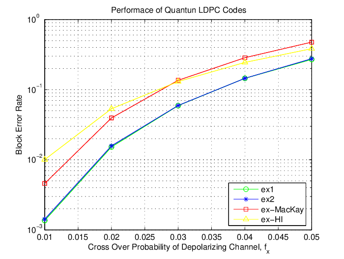
We compare the performance of our examples in section 7.2.1 with these two dual-containing quantum LDPC codes in figure 10. In the simulation, we assume the depolarizing channel and use of sum-product decoding algorithm. The performances of ex1 and ex2 do not differ much. This is not surprising, since these two codes have similar parameters. The reason that the performance of ex-MacKay is worse than our two examples is because there are so many 4-cycles in ex-MacKay. These cycles impair the decoding performance of sum-product algorithm. Our entanglement-assisted quantum QC-LDPC codes also outperform the quantum QC-LDPC code of ex-HI, since the classical QC-LDPC codes used to construct our examples have better distance properties than the classical QC-LDPC of ex-HI. This simulation result is also consistent with our result in [13]: better classical codes give better quantum codes. Even though the parameters are not exactly the same, our codes have higher rate than the code rate of ex-HI.

It is not difficult to verify that the girth of ex1 is 6, and the girth of ex2 is 8. We numerically investigated the performance of these two examples with various numbers of iterations. According to our simulation results, the performance of ex1 and ex2 is almost the same. The result agrees with the classical result in [26] showing that the increase of girth from 6 to 8 is not of great help. The result is quite interesting since it implies that we do not need to worry about constructing QLDPC with higher girth.

7.4 Conclusions

There are two advantages of Type-II QC-LDPCs over Type-I QC-LDPCs. First, according to [54] certain configurations of Type-II QC-LDPC codes have larger minimum distance than Type-I QC-LDPC. Therefore, we can construct better quantum QC-LDPCs from classical Type-II QC-LDPC codes. Second, it seems likely that Type-II QC-LDPCs will have more flexibility in constructing quantum QC-LDPC codes with small amount of pre-shared entanglement, because of the ability to insert zero submatrices. However, further investigation of this issue is required.

By using the entanglement-assisted error correction formalism, it is possible to construct EAQECCs from any classical linear code. We have shown how to do this for two classes of quasi-cyclic LDPC codes (Type-I and Type-II), and proven a number of theorems that make it possible to bound how much entanglement is required to send a code block for codes of these types. Using these results, we have been able to easily construct examples of quantum QC-LDPC codes that require only a relatively small amount of initial shared entanglement, and that perform better than previously constructed dual-containing QLDPCs. Since in general the performance of quantum codes follows directly from the performance of the classical codes used to construct them, and the evidence of our examples suggests that the iterative decoders can also be made to work effectively on the quantum versions of these codes, this should make possible the construction of large-scale efficient quantum codes.

References

[1] S.A. Aly, A. Klappenecker, and P. K. Sarvepalli. Subsystem codes, 2006. quant-ph/0610153.
[2] D. Bacon. Operator quantum error correcting subsystems for self-correcting quantum memories. Phys. Rev. A, 73:012340, 2006.
[3] Dave Bacon and Andrea Casaccino. Quantum error correcting subsystem codes from two classical linear codes, 2006. quant-ph/0610088.
[4] C. H. Bennett, G. Brassard, C. Crépeau, R. Jozsa, A. Peres, and W. K. Wootters. Teleporting an unknown quantum state via dual classical and Einstein-Podolsky-Rosen channels. Phys. Rev. Lett., 70:1895–1899, 1993.
[5] C. H. Bennett, D. P. DiVincenzo, J. A. Smolin, and W. K. Wooters. Mixed state entanglement and quantum error correction. Phys. Rev. A, 54:3824–3851, 1996.
[6] C. H. Bennett and S. J. Wiesner. Communication via one- and two-particle operators on Einstein-Podolsky-Rosen states. Phys. Rev. Lett., 69:2881–2884, 1992.
[7] E. R. Berlekamp, R. J. McEliece, and H. C. A. van Tilborg. On the intractability of certain coding problems. IEEE Trans. Inf. Theory, 24:384–386, 1978.
[8] R. Blume-Kohout, C.M. Caves, and I.H. Deutsch. Climbing mount scalable: Physical resource requirements for a scalable quantum computer. Found. Phys., 32:1641–1670, 2002.
[9] W. Bosma, J.J. Cannon, and C. Playoust. The magma algebra system i: The user language. J. Symb. Comp., 24:235 – 266, 1997.
[10] G. Bowen. Entanglement required in achieving entanglement-assisted channel capacities. Phys. Rev. A, 66:052313, 2002.
[11] S. Bravyi, D. Fattal, and D. Gottesman. GHZ extraction yield for multipartite stabilizer states. J. Math. Phys., 47:062106, 2006.
[12] T. Brun, I. Devetak, and M. H. Hsieh. Catalytic quantum error correction, 2006. quant-ph/0608027.
[13] T. Brun, I. Devetak, and M. H. Hsieh. Correcting quantum errors with entanglement. Science, 314(5798):436–439, 2006.
[14] A. R. Calderbank, E. M. Rains, P. W. Shor, and N. J. A. Sloane. Quantum error correction and orthogonal geometry. Phys. Rev. Lett., 78:405–408, 1997.
[15] A. R. Calderbank, E. M. Rains, P. W. Shor, and N. J. A. Sloane. Quantum error correction via codes over GF(4). IEEE Trans. Inf. Theory, 44:1369–1387, 1998.
[16] A. R. Calderbank and P. W. Shor. Good quantum error-correcting codes exist. Phys. Rev. A, 54:1098–1105, 1996.
[17] T. Camara, H. Ollivier, and J.-P. Tillich. Constructions and performance of classes of quantum ldpc codes, 2005. quant-ph/0502086.
[18] A. C. da Silva. Lectures on symplectic geometry. Springer-Verlag, Berlin, 2001.
[19] M. C. Davey and D. J. C. MacKay. Low density parity check codes over GF(q). IEEE Communications Letters, 2:165–167, 1998.
[20] Yeojin Chung David Poulin. On the iterative decoding of sparse quantum codes, 2008. arXiv:0801.1241.
[21] I. Devetak, A. W. Harrow, and A. Winter. A resource framework for quantum shannon theory, 2005. quant-ph/0512015.
[22] I. Devetak, A. W. Harrow, and A. J. Winter. A family of quantum protocols. Phys. Rev. Lett., 93:239503, 2004.
[23] I. Devetak and A. Winter. Distilling common randomness from bipartite quantum states. IEEE Trans. Inf. Theory, 50:3138–3151, 2003.
[24] D. Fattal, T. S. Cubitt, Y. Yamamoto, S. Bravyi, and I. L. Chuang. Entanglement in the stabilizer formalism, 2004. quant-ph/0406168.
[25] G. David Forney, Markus Grassl, and Saikat Guha. Convolutional and tail-biting quantum error-correcting codes. IEEE Trans. Inf. Theory, 53(3):865–880, 2007.
[26] M. Fossorier. Quasi-cyclic low-density parity-check codes from circulant permutation matrices. IEEE Trans. Inf. Theory, 50(8):1788–1793, 2004.
[27] R. G. Gallager. Low-Density Parity-Check Codes. PhD thesis, Massachusetts Institute of Technology, 1963.
[28] D. Gottesman. Class of quantum error-correcting codes saturating the quantum Hamming bound. Phys. Rev. A, 54:1862–1868, 1996.
[29] D. Gottesman. Stabilizer codes and quantum error correction. PhD thesis, California Institute of Technology, 1997.
[30] Manabu Hagiwara and Hideki Imai. Quantum quasi-cyclic ldpc codes, 2007. quant-ph:0701020.
[31] R. Josza and N. Linden. On the role of entanglement in quantum-computational speed-up. Proc. Roy. Soc. London Ser. A, 459:2011, 2003.
[32] J. Kempe, D. Bacon, D. A. Lidar, and K. B. Whaley. Theory of decoherence-free fault-tolerant quantum computation. Phys. Rev. A, 63:042307, 2001.
[33] A. Klappenecker and P. K. Sarvepalli. Clifford code constructions of operator quantum error correcting codes, 2006. quant-ph/0604161.
[34] E. Knill and R. Laflamme. A theory of quantum error correcting codes. Phys. Rev. A, 55:900–911, 1997.
[35] E. Knill, R. Laflamme, and L. Viola. Theory of quantum error correction for general noise. Phys. Rev. Lett., 84:2525–2528, 2000.
[36] Y. Kou, S. Lin, and M. Fossorier. Low-density parity-check codes based on finite geometries: A rediscovery and new results. IEEE Trans. Inf. Theory, 47:2711–2736, 2001.
[37] D. Kribs, R. Laflamme, and D. Poulin. A unified and generalized approach to quantum error correction. Phys. Rev. Lett., 94:180501, 2005.
[38] David W. Kribs and Robert W. Spekkens. Quantum error correcting subsystems as unitarily recoverable subsystems, 2006. quant-ph/0608045.
[39] R. Laflamme, C. Miquel, J.-P. Paz, and W. H. Zurek. Perfect quantum error-correction code. Phys. Rev. Lett., 77:198–201, 1996.
[40] D. A. Lidar, I. L. Chuang, and K. B. Whaley. Decoherence free subspaces for quantum computation. Phys. Rev. Lett., 81:2594–2597, 1998.
[41] Z. Luo and I. Devetak. Efficiently implementable codes for quantum key expansion. Phys. Rev. A, 75:010303, 2007.
[42] D. J. C. MacKay. Gallager codes that are better than turbo codes. Proc. 36th Allerton Conf. Communication, Control, and Computing, 1998. Monticello, IL.
[43] D. J. C. MacKay. Good error-correcting codes based on very sparse matrices. IEEE Trans. Inf. Theory, 45:399–432, 1999.
[44] D. J. C. MacKay, G. Mitchison, and P. L. McFadden. Sparse-graph codes for quantum error correction. IEEE Trans. Inf. Theory, 50:2315–2330, 2004.
[45] D. J. C. MacKay and R. M. Neal. Near shannon limit performance of low density parity check codes. Electronic Letters, 32(18):1645–1646, 1996.
[46] F.J. MacWilliams and N.J.A. Sloane. The Theory of Error-Correcting Codes. Elsevier, Amsterdam, 1977.
[47] M. A. Nielsen and I. L. Chuang. Quantum Computation and Quantum Information. Cambridge University Press, New York, 2000.
[48] M. A. Nielsen and D. Poulin. Algebraic and information-theoretic conditions for operator quantum error correction. Phys. Rev. A, 75:064304, 2007.
[49] J. Pearl. Propabilistic Reasoning in Intelligent Systems: Networks of Plasusible Inference. Morgan Kaufmann, San Mateo, CA, 1988.
[50] D. Poulin. Stabilizer formalism for operator quantum error correction. Phys. Rev. Lett., 95:230504, 2005.
[51] J. Preskill. Lecture notes for physics 229: Quantum information and computation, 1998. http://www.theory.caltech.edu/people/preskill/ph229.
[52] P. W. Shor. Scheme for reducing decoherence in quantum computer memory. Phys. Rev. A, 52:2493–2496, 1995.
[53] Peter W. Shor. Polynomial-time algorithms for prime factorization and discrete logarithms on a quantum computer. SIAM Journal on Computing, 26(5):1484–1509, 1997.
[54] R. Smarandache and P. O. Vontobel. On regular quasi-cyclic ldpc codes from binomials. in Proc. 2004 IEEE International Symposium on. Information Theory, 2004.
[55] A. M. Steane. Error-correcting codes in quantum theory. Phys. Rev. Lett., 77:793–797, 1996.
[56] W. F. Stinespring. Positive functions on $\mathbb{C}^{*}$ -algebras. Proc. Amer. Math. Soc., 6:211–216, 1955.
[57] R. M. Tanner. A recursive approach to low complexity codes. IEEE Trans. Inf. Theory, pages 533–547, 1981.
[58] W. K. Wootters and W. H. Zurek. A single quantum cannot be cloned. Nature, 299:802–803, 1982.
[59] P. Zanardi. Stabilizing quantum information. Phys. Rev. A, 63:012301, 2000.
[60] P. Zanardi and S. Lloyd. Topological protection and quantum noiseless subsystems. Phys. Rev. Lett., 90:067902, 2003.
[61] P. Zanardi and M. Rasetti. Error avoiding quantum codes. Mod. Phys. Lett. B, 11(25):1085–1093, 1997.

ENTANGLEMENT-ASSISTED CODING THEORY.

Chapter 1: Overview

Chapter 2: Background knowledge

2.1 Single qubit Pauli group

2.2 Multi-qubit Pauli group

2.3 Properties of the symplectic form

Theorem 1.

Proof.

Theorem 2.

Proof.

2.4 Symplectic codes

2.5 Classical quaternary codes

Proposition 1.

Proof.

2.6 Encoding classical information into quantum states

2.6.1 Elementary coding

2.6.2 Superdense coding

2.7 Useful lemmas

Lemma 1.

Proof.

Lemma 2.

Lemma 3.

Proof.

Lemma 4.

Proof.

Chapter 3: Standard quantum error-correcting codes

3.1 Discretization of errors

Theorem 3.

Proof.

3.2 Canonical codes

Proposition 2.

Proof.

Proposition 3.

Proof.

3.3 The general case

Theorem 4.

Proof.

3.4 Relation to symplectic codes

Proposition 4.

Proof.

3.4.1 The CSS construction

Proposition 5.

Proof.

3.5 Examples

3.5.1 The [[9,1,3]][[9,1,3]] Shor code

3.5.2 The [[7,1,3]][[7,1,3]] Steane code

3.6 Discussion

Chapter 4: Entanglement-assisted quantum error-correcting codes

4.1 The channel model: discretization of errors

4.2 The entanglement-assisted canonical code

Proposition 6.

Proof.

Proposition 7.

Proof.

4.3 The general case

Theorem 5.

Proof.

4.4 Generalized construction from quaternary codes

Proposition 8.

Proof.

4.5 Bounds on performance

4.6 Table of codes

Theorem 6.

Proof.

4.7 Discussion

Chapter 5: Operator quantum error-correcting codes

5.1 The canonical code

Proposition 9.

Proof.

Proposition 10.

Proof.

5.2 The general case

Theorem 7.

Proof.

5.3 Discussion

Chapter 6: Entanglement-assisted operator quantum error-correcting codes

6.1 The canonical code

Proposition 11.

Proof.

Proposition 12.

3.5.1 The $[[9,1,3]]$ Shor code

3.5.2 The $[[7,1,3]]$ Steane code