SU-ITP-08-12
OIQP-08-06
UCB-PTH-08-60
Future Foam
Raphael Bousso 1, Ben Freivogel 1, Yasuhiro Sekino 2,3, Stephen Shenker 3,
Leonard Susskind 3, I-Sheng Yang 1, and Chen-Pin Yeh 3
Department of Physics and Center for Theoretical Physics, University of California, Berkeley,
and Lawrence Berkeley National Laboratory, Berkeley, CA 94720, U.S.A.
Okayama Institute for Quantum Physics, Okayama 700-0015, Japan
Physics Department, Stanford University, Stanford, CA 94305, U.S.A.
We study pocket universes which have zero cosmological constant and non-trivial boundary topology. These arise from bubble collisions in eternal inflation. Using a simplified dust model of collisions we find that boundaries of any genus can occur. Using a radiation shell model we perform analytic studies in the thin wall limit to show the existence of geometries with a single toroidal boundary. We give plausibility arguments that higher genus boundaries can also occur. In geometries with one boundary of any genus a timelike observer can see the entire boundary. Geometries with multiple disconnected boundaries can also occur. In the spherical case with two boundaries the boundaries are separated by a horizon. Our results suggest that the holographic dual description for eternal inflation, proposed by Freivogel, Sekino, Susskind and Yeh, should include summation over the genus of the base space of the dual conformal field theory. We point out peculiarities of this genus expansion compared to the string perturbation series.
1 Introduction
The nonperturbative definition of string theory in asymptotically flat or anti-de Sitter (AdS) spacetimes is now basically understood. Matrix theory [1] and AdS/CFT correspondence [2] provide concrete non-perturbative (holographic) formulations of quantum gravity in terms of non-gravitational gauge theories. These theories taught us many things. For instance, the fact that formation and evaporation of a black hole is mapped to a manifestly unitary process in gauge theory makes us strongly believe that information is not lost in black holes.
On the other hand, it is not yet clear how to define an exact quantum theory for a cosmological, or inflating, spacetime. The main source of difficulty seems to be the fact that there is no obvious asymptotic region where interactions are turned off.
Finding a non-perturbative framework for cosmology is especially important because of the existence of the string landscape [3]: string theory contains a large number of vacua including metastable de Sitter vacua. Metastability is an approximate concept. Even though there is strong evidence for the existence of the landscape, which is obtained from the low-energy effective theory analysis, the meaning of these metastable vacua is not totally clear until we have an exact theory.
In the landscape, bubbles (universes in different vacua, or “pocket universes”) are created by tunneling. Eternal inflation generically occurs. Here the false vacuum inflates so fast that bubbles of true vacuum cannot percolate and the physical volume of the space remains dominated by the false vacuum forever. Infinitely many bubbles are produced, and the volume inside each bubble is also infinite. It is not known how to regulate these infinities. This is related to the measure problem. If we can find a non-perturbative framework, it may give some clues about this problem.
In [4], a holographic dual description for eternal inflation was proposed. The authors consider an FRW universe with zero cosmological constant (c.c.) created by tunneling from de Sitter space. The tunneling is described by the Coleman-De Luccia (CDL) instanton [6], which tells us that the FRW universe is an open universe whose constant time slices are 3-dimensional hyperboloids. The dual theory is a conformal field theory (CFT) defined on at the boundary (spatial infinity) of the 3-hyperboloid (Figure 1).

In this “FRW/CFT duality,” the dual theory contains 2-dimensional gravity (the Liouville field). One may wonder why gravity is not decoupled on the boundary, as in AdS space where it is fixed with a boundary condition. The reason for non-decoupling is that the FRW universe is embedded in de Sitter space. Our boundary is alternately regarded as the bubble wall at future infinity of de Sitter space (see Figure 1). In de Sitter space, fluctuations produced at early time are stretched by inflation and cannot be smoothed out by late-time fluctuations, so the fluctuations at two points remain correlated after those points go out of causal contact (see e.g. [7]). The gravity fluctuations on the boundary of the FRW universe is of the same origin. Indeed, the graviton correlator computed in [4] using the Euclidean prescription remains finite as the points approach the boundary of the FRW universe. A boundary such as this one where gravity is not decoupled is called a “warm” boundary [5], as opposed to the “cold” boundary of (global) AdS space. In most proposals for a holographic duality for inflation, such as the dS/CFT correspondence [9] and the dS/dS correspondence [10], gravity is not decoupled.
In addition to the above perturbative argument, bubble collisions which are inevitable in eternal inflation indicate that the boundary geometry is fluctuating. Consider a collision of two bubbles of the same vacuum, for which no domain wall remains after the collision. The bulk space will approach a smooth geometry. If the c.c. of the vacuum is zero, a timelike observer can see the whole space inside the bubbles eventually; the geometry contains only one “hat” (future asymptotics of flat space). However, the boundary geometry will be deformed from a perfect sphere. It is conjectured that a bubble collision corresponds to an instanton in the dual theory [4].
In this paper, we point out that the boundary is not only “metrically warm,” but is also “topologically warm.” A universe with a non-trivial boundary topology can arise from bubble collisions. We can easily imagine a “ring” that appears as a result of collisions of three or more bubbles (Figure 2). The region “in the middle” does not close up if its size is larger than the horizon scale. Even though the wall of the true vacuum moves outwards, the inflation of de Sitter space surpasses it. A timelike observer in the true vacuum (the “bulk” of the torus) can eventually see the whole boundary, as we discuss in section 2. Boundaries with general higher topologies will also be present.

Non-trivial topologies are suppressed by powers of the nucleation rate , compared to the spherical topology, and may not be important observationally. However to define the holographic theory we should include everything that a single observer can see. This means that we should sum over topologies of the 2-dimensional space on which the CFT is defined.
Summation over topologies is reminiscent of string perturbation theory, which is an asymptotic expansion. The string perturbation series does not converge, and important objects, such as D-branes, cannot be seen in a perturbative expansion. We might wonder whether a similar thing happens in the genus expansion in our dual theory. We will estimate the growth of terms in the series by taking the sum over bubbles, and argue that here the series converges.
We also note that bubble collisions can produce spacetimes with multiple boundaries. This happens when the bubbles form a “shell,” for example. If two boundaries are accessible to a single timelike observer, it would be confusing in terms of the dual theory. For the case of two spherical boundaries, we can show that the two boundaries are causally disconnected. It would be very interesting to know whether this generalizes to cases with more complicated topology, so that a given observer can only see a single connected boundary.
This paper is organized as follows: In section 2, we explain that universe with non-trivial topology can be produced by bubble collisions. We first give a general argument based on the assumption that bubble walls turn into a wall of dust after colliding. We then perform analytic study in the thin-wall approximation, for the two limiting cases with torus topology. We first consider bubbles aligned on a straight line with equal spacing, and obtain asymptotic geometry after collisions. We then consider a “coarse grained” version, in which we approximate the domain wall between the true and the false vacuum regions by a smooth torus. In section 3, we show that there can be a universe with multiple boundaries. We study the case where the true vacuum is inside a shell-like region, and see that a singularity develops inside the shell, leaving two boundaries causally disconnected. In section 4, we discuss implications of the non-trivial boundary topology for the dual theory. We study large order behavior of the genus expansion, and discuss possible interpretation in the dual CFT.
2 Boundary with non-trivial topology
We shall consider the simplest setting in this paper: Gravity is coupled with a scalar field whose potential has two minima, a false vacuum with positive c.c. and a true vacuum with zero c.c. We consider four spacetime dimensions.
If the space is filled with false vacuum, bubbles of true vacuum will be nucleated with a rate which is calculated from the CDL instanton [6]. We are interested in diagnosing the topology of the boundary between the true vacuum and the false vacuum at conformal infinity. Before taking true vacuum bubbles into account, conformal infinity of de Sitter space is a 3-sphere. When a bubble of true vacuum nucleates, it eats up a ball out of the conformal infinity of de Sitter space. The size of the ball depends on the time of nucleation. The boundary of the true vacuum region is the boundary of the ball, a 2-sphere. When two bubbles of true vacuum collide in de Sitter space the region of de Sitter conformal infinity which is removed is simply given by superposing the two balls from each nucleation. The geometry inside the balls may be complicated, and depends on the physics of what happens when the walls collide. However, the boundary between de Sitter space and the true vacuum is simply given by superposing balls of different sizes, one for each true vacuum bubble, and then looking at the boundary of this region. It is possible that the nucleated bubbles collide and form a ring (or “chain of pearls”; see Figure 2) where the true vacuum is inside a torus, or in a similar fashion anything with higher genus.
An important question is whether a single observer inside the true vacuum can see the entire boundary. To answer this question, it is necessary to construct the geometry inside the true vacuum regions. As we mentioned above, the geometry depends on the physics of what happens when the domain walls collide. We first demonstrate the existence of a boundary of arbitrary genus, all of which is visible to a single observer in the true vacuum region, using a simplified “dust” model in section 2.1. Then using a somewhat more realistic “radiation shell” model we construct the smooth solution in the simplest case, a torus, in Section 2.2 and 2.3. Finally in Section 2.4, we make a conjecture about the smooth geometry inside a boundary of any genus based on our torus solution.
2.1 Chain of pearls with dust walls
For the moment, we assume that when two bubbles collide, their domain walls annihilate into a (2+1) dimensional wall of dust. In other words, we assume that there is a type of “domain wall” with equation of state separating the two regions of true vacuum after the bubbles collide. The resulting geometry for a single collision was constructed in [11]. The entire true vacuum region is within the backward lightcone of a single observer. With more collisions, as long as the resulting dust walls do not cross each other, we can iterate the same solution and show that the entire interior region is causally connected. The non-trivial question is, can the dust walls stay away from each other for the collisions necessary to make true vacuum regions of various topologies? We will find that connected boundaries of arbitrary topology can be constructed using this simple procedure, but disconnected boundaries cannot be constructed in this way.
Consider a given true vacuum bubble which collides with several other true vacuum bubbles. We need to know whether the dust walls from these various collisions intersect each other. In the thin wall approximation, the interior of each bubble is the Milne universe out to the dust walls, with metric
| (2.1) |
where is the metric on 3-dimensional hyperbolic space. The conformal boundary of is a 2-sphere. This is the boundary between de Sitter space and Minkowski space for a single bubble.
Now consider collisions. A given collision destroys part of the original boundary. At conformal infinity, when two true vacuum balls overlap, the part of each which is inside the other ball is destroyed. Focusing on a given bubble, collisions punch holes in the boundary . These holes are the interiors of circles, because the overlapping ’s intersect in a circle. The destroyed pieces of domain wall have been converted to dust walls. Our concern is whether these dust walls intersect.
Studying the dynamics of the dust walls gives the result that at late time in the coordinates (2.1) the dust wall asymptotes to the minimal surface inside whose boundary is the intersection circle [11] . This minimal surface is simply an with unit radius. (At earlier times, the dust wall is not yet a minimal surface, but we are interested in late time because the dust wall extends maximally far into the space at .) Now if a given bubble collides with several other bubbles, then there are several dust walls emanating from the intersection circles. The minimal surfaces (dust walls) intersect if and only if the different intersection circles intersect each other.
So we have a simple rule for building a large class of solutions in which the entire true vacuum region is causally connected. Start with de Sitter conformal infinity, which is an , and put down balls of true vacuum of any size in any location. The boundaries of the balls are ’s, which when they intersect generically intersect in circles. The only rule is that the intersection circles cannot intersect each other.
(It is not obvious from our analysis here, but the dust walls intersect if and only if the collision ’s intersect. When this happens black holes generically form [12], so the analysis becomes difficult no matter what assumption we make for the physics of the collision.)
Now what kinds of interesting boundary topologies can be constructed in this way? It is possible to connect geometries with arbitrary connected boundary using this construction. For example, we can construct a true vacuum region of torus topology, as shown in Figure 2. Since the true vacuum regions overlap only pairwise, the intersection circles are all well separated from each other, and our construction works.
On the other hand, it is not possible to construct geometries with disconnected boundaries using this technique. The boundary of the true vacuum region is constructed out of a number of ’s which are glued together along circles. The interiors of the circles are holes in the ’s. Since the circles do not intersect in this construction, it is possible to get from one point along a given holey to any other point. Also, it is possible to move from one holey to one connected to it by moving across the gluing circle. Therefore, the boundary of the true vacuum region is connected.
2.2 Sequence of collisions
We now turn to a more detailed analysis of bubble collisions where we make the somewhat more realistic assumption that all energy is liberated in a shell of radiation.
For simplicity, we would like to start with as many symmetries as possible. A de Sitter space with one bubble has SO(3,1) symmetry; this is inherited from the spherical symmetry SO(4) of the Euclidean CDL instanton [6]. When there are two bubbles, the direction connecting the centers of the bubbles singles out a preferred direction, but there is SO(2,1) residual symmetry. When there are four or more bubbles, there is generically no residual symmetry. However, if nucleation sites are on the same spacelike geodesic ( the great circle of the minimal ), SO(2,1) symmetry is preserved. In addition, the circle of nucleation points gives us a discrete subgroup of , so we have which contains a torus.
We will use coordinates with manifest SO(2,1) symmetry [13, 12]. De Sitter space can be written as
| (2.2) |
with
| (2.3) |
where is the de Sitter radius (the horizon size)11 1 The de Sitter metric (2.3) is obtained by parameterizing the embedding coordinates in R4,1 (which satisfy ) as follows: (where , and ), , . The configuration considered here is invariant under SO(2,1) acting on the space. The metric (2.3) does not cover the whole de Sitter. To study the trajectory in the directions other than , it is more convenient to use global coordinates (2.15)., and . The bubbles are nucleated at time , along the circle in the direction. For simplicity, we assume that the nucleation sites are evenly spaced with distance . (We are assuming is an integer.) The initial size of a bubble is determined by the parameters of the scalar potential.

The profile of bubble walls in the () plane will be as depicted in Figure 3. In the thin-wall limit, geometry in each bubble is flat. We parametrize flat space in such a way that factor is manifest, which is of the form (2.2) with . We patch it to de Sitter space on the domain wall. Since the metric component along the wall should be continuous across the wall, the coordinate (which sets the scale for the metric) should have the same value when we approach the domain wall from either side. The coordinate for the flat and the de Sitter side will be different. The trajectory of the domain wall is determined by the Israel junction condition once the equation of state for the domain wall is given.
Bubble collisions occur along an . To find the metric after collision, we make an assumption following [13, 12]: When two bubbles collide, the bubble walls disappear instantaneously and turn into radiation. Radiation follows a light-like trajectory in the space. The geometry in the region behind the radiation differs from flat space in general, since the radiation carries away some energy. The metric will be of the form (2.2) with
| (2.4) |
This is the most general zero-c.c. geometry with symmetry; it is the hyperbolic version of the Schwarzschild geometry. The causal structure of this metric is given in Figure 4. There is a time-like singularity at , but as we will see, only the () region is relevant for us.
The parameter is determined by the following condition [12]. To make the formula simple, let us ignore the initial size of each bubble so that the bubble walls are moving at the speed of light. When two light-like domain walls collide and emit two light-like domain walls (i.e. walls of radiation), spacetime is divided into four regions. We will label them I, II, III, IV in the way depicted in Figure 4, and denote the function in those regions by and so on. At the time of the collision (which is common in all the regions), they satisfy
| (2.5) |
This is essentially the energy conservation condition [15]. Substituting de Sitter metric (2.3) for and flat metric for and , we find
| (2.6) |
The region IV is the part of the metric (2.4), and the above equation implies . Thus, there is no singularity in region IV.

The collision time is determined by the initial condition. In terms of the conformal coordinate , defined by , bubbles separated by a distance collide in a time . If the separation at the nucleation time is small, , we can approximate , and get . In this limit, the condition (2.6) becomes
| (2.7) |
Geometry of the region IV is maximally curved at the earliest time, , where the deviation of from 1 is
| (2.8) |
This can be made arbitrarily small by making small.
As we see from Figure 3, a wall of radiation collides with another one which comes from the neighboring collision. Again, walls of radiation are emitted at the collision, and the metric behind the radiation is changed. This process will be repeated infinite times.
The geometry after such collisions is obtained by using the junction condition iteratively. Let us call the function after -th collision (which means this and ) and write it
| (2.9) |
Also we define to be the time of -th collision (the above is ). The condition (2.5) gives us
| (2.10) |
There is another condition which says that the coordinate distance traveled by the light between -th and -th collisions is equal to the one between -th and -th collisions:
| (2.11) |
These recursion relations simplify when the metric is close to flat. If , , are all much smaller than 1, the leading part of (2.10) and (2.11) becomes
| (2.12) | |||||
| (2.13) |
Together with our initial conditions, , , and , these give us
| (2.14) |
When , the deviation from the flat metric is always small, , so our approximation is consistent.
We can compute corrections by substituting this leading order solution into (2.10), (2.11) and solving them perturbatively in . The function decreases at subleading order22 2 This expression is valid when is sufficiently small. At some point the error accumulates and this lowest order approximation breaks down. as . The geometry asymptotically approaches flat space locally, although the logarithmic rate of approach is slower than the rate for the ordinary collision of two bubbles. Numerical solutions obtained by iteration (without assuming ) indeed shows that the function decreases logarithmically for large (See Figure 5). We can also see that the maximum value of decrease as we make small, so our perturbative analysis can always work by making this control parameter small.
There is an useful physical picture for the above analysis. If there is no incoming radiation, Eq. (2.9) will approach flat space locally. The leading order analysis shows that for an observer, the radiation walls keep arriving at equal time intervals, therefore they serve as a constant reminder of non-flatness. The perturbative correction and the simulation suggest that radiation walls actually arrive at increasing time intervals, which guarantees flatness at future infinity.


Taking the smooth () limit, we have exact symmetry, the boundary of the flat region has two non-contractible circles. In the global coordinates for de Sitter,
| (2.15) |
the above solution looks like the future lightcone of the axis circle at . In general we can also consider a circle at . At future infinity, the bubble wall (radial light ray from ) reaches . One of the circles of the torus has radius . This is the circle ( direction) contained in one bubble. The other circle of the torus is in the -direction which traverses many bubbles, and has radius , Asymptotic ratio of the two radii is
| (2.16) |
We established the asymptotic local flatness for the case, in which even though becomes infinite but remains finite and equals to the horizon size . For , also grows to infinity. Each source of radiation (the collision ) is moving away from each other. This should make the approach to flat space faster. We should be able to patch flat space to de Sitter across a toroidal domain wall. We will study this in the next subsection.
2.3 Coarse grained smooth torus
We will construct the smooth torus solution suggested in the previous subsection, which is more general since it has only symmetry.
To make the symmetry manifest, we express the global de Sitter space as
| (2.17) |
where , and . 33 3 This metric is obtained by parameterizing the embedding coordinates in as , , , , . The relation of these coordinates to the usual global time, defined by , is: .
For the interior flat space, we start from the Minkowski space with a manifest ,
| (2.18) |
By identifying the space under , and redefining the coordinates, , , we get
| (2.19) |
The conical singularity at is not a problem for us; we do not extend the solution to infinite past, and this singularity is in the unphysical region, as we will see shortly.
The torus boundary between the de Sitter space and the flat space is a surface parametrized by . The induced metric,
| (2.20) |
should have the same form, when we approach the domain wall from either side, (2.17) or (2.19).
We take the plus sign in (2.21), and consider the part to be physical. At , we have , and takes the minimum value . (We loosely call the nucleation time of the torus bubble.) The parameter corresponds to the tension of the domain wall, and is the limit of zero tension domain wall, as we will see below.
Another parameter controls the global time at the nucleation. The limit corresponds to late nucleation, and the limit corresponds to nucleation at the minimal , which should correspond to the case studied in the last subsection. The asymptotic aspect ratio of the two circles of the torus is given by . In the limit, the ratio is infinite. is constant , while grows to infinite size; this is the situation we mentioned at the end of the last subsection.
The junction condition (see Appendix B) tells us that we need the following (2+1) dimensional stress tensor on the domain wall:
| (2.22) | |||||
| (2.23) |
Ordinary domain wall, which is made from a kink of scalar field, has , where is the tension determined by the shape of the scalar potential. Here we have extra term proportional to , but since it decreases as the torus grows, we should probably set
| (2.24) |
The fact that we need non-standard stress energy on the domain wall is not surprising. We expect this solution to be an effective description for a large number of spherical bubbles collided with each other. In the exact description (as the one in the last subsection), there is no translational symmetry in one () direction. The translational symmetry appears after smearing over the direction, but before smearing, there would be defects which lie along the direction (and are symmetric along ). The form of the extra terms, , , is what we expect for such a string-like object wrapped along .
2.4 Boundary with higher topologies
The above analysis shows the existence of bubbles (true vacuum region) with torus boundary. We believe boundaries of any genus can appear in the radiation shell case as well as in the dust case discussed at the beginning of this section.
A configuration with genus 2 or larger typically involves “Y-shape” collisions where three bubbles collide with another bubble in the middle. To understand the qualitative behavior of this type of collision, we will use intuition from the analysis of SO(2,1) symmetric chain of collisions for the torus case. Local geometry that results from each collision will be roughly the one studied in Section 2.2. Even though we do not have the symmetry now, if the geometry is close to flat, we will be able to use Newtonian approximation, and add the effect of each collision. In the middle bubble of the Y-shape collision, radiation shells will arrive more often than in the torus case (since radiations come from three directions rather than two). This may effectively shorten the interval between successive radiation. (which corresponds to in Section 2.2). However, this does not change the fact that further radiation shells arrive at an increasing interval, which is enough to guarantee that locally the metric approaches Minkowski space.
The candidate for the asymptotic geometry of the flat region would be the following:
| (2.25) |
where is the metric of a 3-dimensional space obtained by modding out by elements of a suitable discrete subgroup (the Schottky group). See e.g., [16]. Negatively curved space with one boundary with any genus and arbitrary value of moduli parameters can be realized this way. For example, the torus geometry (2.18) in the last subsection is equivalently represented44 4 Poincaré coordinates in (2.26) are related to the coordinates in (2.18) by , , . Translation corresponds to a dilatation by . as a quotient of ,
| (2.26) |
under a scale transformation with a given (). This transformation has two fixed points, at origin and at infinity. By further modding out the space by transformations which have different sets of fixed points and parameters corresponding to , we get a higher genus boundary. The number of transformations applied corresponds to the genus . Any value of the moduli can be realized by choosing the parameters of the scale transformations [16]. We expect the initial condition produced by bubble collisions to evolve into this geometry embedded in de Sitter space.
The flat region constructed above is causally connected (i.e. a time like observer in the flat region can eventually see the whole region). This is clear from the fact that the whole space of an open universe with zero c.c. is causally connected, and that taking a quotient only makes causal contact easier.
This suggests that we should sum over the topology of the boundary on which the holographic dual theory is defined. We will discuss implication of the higher genus boundaries in Section 4. Before that, in the next section we mention an example of geometry which has disconnected boundaries, which is a little confusing in terms of holographic duality.
3 Multiple boundaries
Bubble collisions can also produce configurations which have multiple boundaries. In this case, the dust wall model in Section 2.1 does not guarantee the existence of a smooth geometry, since dust walls must cross each other to form multiple boundaries. Actually, in Section 3.1 we will show that two spherically symmetric boundaries must be causally disconnected. Cases with higher genus are less clear and will be discussed in Section 3.2.
3.1 Two spherical boundaries
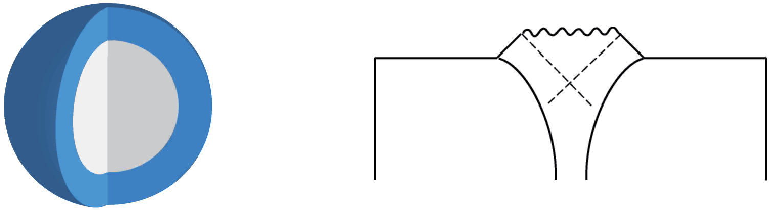
It could happen that bubbles form a “shell” rather than a ring (see Figure 6). Let us assume that a large number of bubbles are nucleated on a sphere, and approximate the geometry with a spherically symmetric one. The space is divided into three regions. The flat region is in a thin shell, and it has two disconnected spherical boundaries. Let us assume both de Sitter regions are larger than their horizon size.
This initial condition will evolve into a geometry whose Penrose diagram is shown in Figure 6 [17]. From Birkhoff’s theorem, in our spherical symmetric situation, the geometry of the flat region should be the Schwarzschild geometry. The size of the two spheres (boundaries) should increase, since they are larger than de Sitter horizon. The junction condition tells us that the zero c.c. space is always “inside” de Sitter space, i.e., the former is on the side that the area of decreases. Domain wall with such properties has to be in the “white hole” region of the Schwarzschild geometry. Patching de Sitter and Schwarzschild geometries, we get Figure 6.
The Schwarzschild mass is determined so that the initial condition satisfies the junction condition. In the simplest case where bubbles with negligible size are nucleated along which has radius (we assume the is at the “center” of of global de Sitter), the mass will be [17]
| (3.1) |
We can get this by studying the junction condition at the “nucleation time” (when the domain walls have zero radial velocity), in the limit of small tension (in this limit the radii of the two ’s are almost equal to )55 5 The junction condition is given e.g. in [22]. In the “static” coordinates used in [22], the coordinate (which gives the size of ) is timelike in the region of interest where is larger than the horizon size. The at rest at the center of the global corresponds to . Substituting this into their junction condition, and setting the domain wall tension zero, we get (3.1)..
The two asymptotic regions are separated by horizons. A timelike observer who reaches timelike infinity can see only one boundary. That observer will feel like there is a black hole in the interior. This black hole will eventually evaporate, leaving two disconnected geometries. Each geometry has one spherical boundary. They will relax to flat space.
The holographic dual theory is expected to describe the region that a single observer can see. The above geometry (at least at late time) will correspond to a perturbation in the dual theory, similar to the one corresponding to a black hole in FRW universe.
3.2 More general cases
Bubble collisions can also produce configurations which have multiple boundaries with higher topologies.
For example, consider two toroidal boundaries: assume there is a torus inside a torus, and true vacuum fills the region between the two tori. If this torus is long and thin, it can be approximated by infinite straight tubes; de Sitter space fills inside the inner tube and outside the outer tube. We assume the radii of the inner and outer tubes are both larger than the de Sitter horizon radius.
It is not obvious how this geometry evolves. The geometry of the true vacuum region will not simply be a flat space with conical deficit, as in the case of cosmic string (or the dimensionally reduced 2+1 D gravity). If we imagine a cosmic string with tension given by the energy of the de Sitter region (in the tube of radius ), its tension would be , when the de Sitter region is larger than the horizon size . Cosmic string with such a large tension cannot exist, since it corresponds to a deficit angle larger than . In fact, the problem is not purely (2+1) dimensional, since we have an extra degree of freedom (the metric component along the tube). So the geometry will not be just flat in general. Possibly, a singularity forms in the true vacuum region, or instability occurs and inner de Sitter meet with outer de Sitter.
A flat region with multiple disconnected boundaries would be confusing in terms of the holographic duality. This would mean that CFT’s defined on each boundary are not independent and somehow coupled. It is not clear how to couple two CFT’s without introducing explicit coupling. This is the issue raised in [18] for asymptotically Euclidean AdS spaces with multiple boundaries.
We have seen that, at least for the case of spherical boundary, a timelike observer can see only one boundary. So far we do not have a clear conclusion for higher genus cases66 6 We have not ruled out the possibility that the true vacuum region with two genus boundary asymptotes to a constant curvature geometry, modded out by “(quasi-)Fuchsian group,” studied in [18].. This point clearly deserves further study.
4 Summing over boundary topologies
The authors of [4] proposed a holographic dual description for a bubble with spherical boundary. The proposal is that the dual theory is a CFT defined on the boundary, and that the boundary metric (the Liouville field) should be integrated. Results in the above sections, which show the existence of boundaries with non-trivial topology, imply that we have to sum over the topology of the base space on which the dual CFT is defined. This suggests that eternal inflation is described by a kind of “string theory.” The CFT has and is coupled to Liouville, and so it is a “supercritical” string theory.
How should each topology be weighted? i.e., what is the string coupling ? Adding a handle requires a minimal number of extra bubbles, (which might be two or three). It seems appropriate to identify the coupling constant as .
From the string theory point of view there are a number of peculiarities in the sum over topologies. First, to nucleate a torus with a modulus corresponding to a large aspect ratio () requires many bubbles to be nucleated. This means that this region of moduli space is strongly suppressed by a factor that looks roughly like . This is surprising. “Pseudotachyons” typically appear in supercritical strings [19, 20]. They will cause an IR divergence at . Also there is no extra dependence in the genus one amplitude.
From the bubble nucleation point of view it seems that the sum over higher topologies is convergent. All configurations of connected bubbles can be thought of as a branched polymer with nodes. There are order such configurations (where is a constant of order one). So the sum over them appears to be convergent. The higher genus contributions are a systematically small part of the sum.
This is surprising from the string theory point of view. There the integral over moduli space of genus typically goes like indicating a divergent series and characteristic nonperturbative effects of size [21].
We do not have a full understanding of these differences. We can point to one novel aspect of the “string theory” of [4] which might be relevant. The central charge is argued to be where is the ancestor de Sitter entropy [4, 5]. Nucleation rate is . So, roughly speaking, . The world-sheet parameters of the string theory are linked to the string coupling.
Acknowledgements
We thank Tom Banks, Simeon Hellerman and Eva Silverstein for helpful discussions. The work of YS is supported in part by MEXT Grant-in-Aid for Young Scientists (B) No.19740173. SS, LS, and CY are supported in part by NSF Grant 0244728. RB, BF, and IY are supported by the Berkeley Center for Theoretical Physics, by a CAREER grant of the National Science Foundation, and by DOE grant DE-AC0376SF00098.
Appendix A Domain wall trajectory
In this appendix, we solve the Israel junction conditions to find a solution which consists of a toroidal domain wall separating de Sitter space from Minkowski space.
The trajectory of the domain wall satisfies the following two equations:
| (A.1) | |||||
| (A.2) |
where the dot denotes the derivative w.r.t. the proper time .
We can combine them and use to get a first order differential equation
| (A.3) |
Solving it as a quadratic equation first, we have
| (A.4) |
Changing the variable to , we get a simple differential equation,
| (A.5) |
with the solution
| (A.6) |
where is an integral constant. We will take the plus sign, since this corresponds to the case of interest where both and are growing.
Appendix B Junction conditions
In this appendix we review the Israel junction conditions and compute the extrinsic curvature for the case of interest, a toroidal domain wall.
The D stress tensor of the domain wall is related to the jump in extrinsic curvature (see e.g., [22]),
| (B.1) |
| (B.2) |
To calculate the extrinsic curvature, it is convenient to write down the Gaussian normal coordinate in the vicinity of the domain wall. Suppressing the symmetric directions , we need a coordinate transformation . 77 7 Here (and only here) we use the printed to denote as the coordinates (independent variables), as opposed to , which is a given function of the coordinate . In the following, we will abbreviate the latter as , since we believe its meaning is clear from the context.
| (B.3) |
where is the domain wall and is the unit vector orthogonal to it.
On the flat space side, we have
| (B.4) |
and the Gaussian normal coordinate is
| (B.5) |
We ignore the higher order terms in Eq. (B.3), which will not be needed for the calculation of the extrinsic curvature,
| (B.6) |
| (B.7) |
References
- [1] T. Banks, W. Fischler, S.H. Shenker and L. Susskind, Phys.Rev.D55:5112-5128,1997, hep-th/9610043.
- [2] J. M. Maldacena, Adv.Theor.Math.Phys.2:231-252,1998, Int.J.Theor.Phys.38:1113-1133,1999, hep-th/9711200.
- [3] R. Bousso and J. Polchinski, JHEP 0006:006,2000, hep-th/0004134; L. Susskind, in Carr, Bernard, (ed.), Universe or multiverse? 247, hep-th/0302219; M. R. Douglas and S. Kachru, Rev.Mod.Phys.79:733, 2007, hep-th/0610102.
- [4] B. Freivogel, Y. Sekino, L. Susskind and C.-P. Yeh, Phys.Rev.D74:086003,2006, hep-th/0606204.
- [5] L. Susskind, arXiv:0710.1129 [hep-th].
- [6] S. R. Coleman and F. De Luccia, Phys.Rev.D21:3305,1980.
- [7] A. .D. Linde, Particle physics and inflationary cosmology, Harwood Academic, 1990.
- [8] A. H. Guth and E. J. Weinberg, Nucl.Phys.B212:321,1983.
- [9] A. Strominger, JHEP 0110:034,2001, hep-th/0106113; J. M. Maldacena, JHEP 0305:013,2003, astro-ph/0210603.
- [10] M. Alishahiha, A. Karch, E. Silverstein and D. Tong, AIP Conf.Proc.743:393-409,2005, hep-th/0407125; M. Alishahiha, A. Karch and E. Silverstein, JHEP 0506:028,2005, hep-th/0504056.
- [11] R. Bousso, B. Freivogel and I.-S. Yang, Phys.Rev.D74, 103516, 2006, hep-th/0606114.
- [12] I. G. Moss, Phys.Rev.D50: 676, 1994.
- [13] S. W. Hawking, I. G. Moss and J. M. Stewart, Phys.Rev.D26:2681,1982.
- [14] B. Freivogel, G. T. Horowitz and S. Shenker, JHEP 0705:090,2007, hep-th/0703146
- [15] D. Langlois, K.-i. Maeda and D. Wands, Phys.Rev.Lett.88:181301, 2002, gr-qc/0111013.
- [16] K. Krasnov, Adv.Theor.Math.Phys.4:929, 2000, hep-th/0005106.
- [17] K. Sato, H. Kodama, M. Sasaki and K. Maeda, Prog.Theor.Phys.65:1443,1981; Prog.Theor.Phys.66:2052,1981; Phys.Lett.B108:98,1982; Phys.Lett.B108:103,1982.
- [18] J. M. Maldacena and L. Maoz, JHEP 0402:053,2004, hep-th/0401024.
- [19] O. Aharony and E. Silverstein, Phys.Rev.D75:046003, 2007, hep-th/0612031.
- [20] S. Hellerman and I. Swanson, Phys.Rev.D77:126011,2008, hep-th/0611317.
- [21] S. H. Shenker, in Cargese 1990, Proceedings, Random surfaces and quantum gravity 191-200.
- [22] S. K. Blau, E. I. Guendelman, A. H. Guth, Phys.Rev.D35:1747,1987.