Mmmmm DD, YYYY
Dynamical vertex approximation
Abstract
We give an elementary introduction to a recent diagrammatic extension of dynamical mean field theory (DMFT) coined dynamical vertex approximation (DA). This approach contains the important local correlations of DMFT, giving, among others, rise to quasiparticle renormalizations, Mott-Hubbard transitions and magnetism, but also non-local correlations beyond. The latter are at the very essence of many physical phenomena in strongly correlated elecectron systems. As correlations are treated equally on all length scales, DA allows us to describe physical phenomena such as magnons, quantum criticality, and the interplay between antiferromagnetism and superconductivity. We review results hitherto obtained for the Hubbard model in dimensions , 2, and 1.
1 Introduction
Dynamical mean field theory (DMFT) [1, 2, 3, 4] has been a success story for the theoretical modeling of strongly correlated electrons systems since it contains the major contribution of electronic correlations: the local ones. Diagrammatically, DMFT corresponds to all topologically distinct Feynman diagrams, albeit only for their local part. Hence, it is a non-perturbative approach which, from another point of view, can be envisaged as a mean-field theory where the local Coulomb interaction on all sites but one is replaced by a dynamical (frequency-dependent) mean field given in terms of the self energy . First, DMFT was applied to model Hamiltonians for studying, among others, the Mott-Hubbard transition [2, 3, 5], magnetism [6, 7, 8, 9, 10], and the strong quasiparticle renormalization of correlated electrons, including the only recently observed kink in the quasiparticle’s dispersion relation [11, 12, 13]. In the last years, the focus shifted towards the realistic calculation of material properties [14, 15, 16, 17, 18] and the inclusion of non-local correlations, which are the topic of our paper.
While usually smaller in absolute terms than the local correlations, the non-local correlations nonetheless become essential at low temperatures where they lead to pertinent correlation effects such as spin fluctuations, magnons, quantum criticality, and (possibly) superconductivity. Actually, many of the most fascinating phenomena of strongly correlated electron systems are driven by non-local correlations.
Two different paths have been followed to extend DMFT by non-local correlations, see Fig. 1.

cluster extensions of DMFT diagrammatic extensions of DMFT


Cluster extensions consider instead of the single DMFT site (the local problem or Anderson impurity model) a couple of sites and take correlations between these sites into account, see Ref. \citenreview for a review. There are two main variants: cellular (or cluster) DMFT [20, 21, 22] where the self energy is directly related to a supercell in real space, and the dynamical cluster approximation (DCA) [23, 24, 25, 21] where it is patched in space. A generalization in form of a self energy functional approach has been formulated more recently by Potthoff [27, 28]. Also the expansion of DMFT [29, 30] can be subsumed here since it connects a single-site cluster and a two-site cluster. These approaches have been applied successfully for studying the one-dimensional [31, 32] and two-dimensional [33, 21, 34, 35, 19] Hubbard model, as well as for the investigation of spin-Peierls physics in Ti2O3[36], NaV2O5 [37], and VO2 [38]. The biggest drawback of the cluster extensions is their restriction to short-range correlations because the numerical effort is exponentially growing with the number of cluster sites, similar to the direct quantum Monte Carlo simulation[39] of the lattice problem. For the one-band Hubbard model, approximately 30-60 sites are possible which means a correlation length of about 3 sites in two dimensions and 1 site in three dimensions. In realistic multi-orbital calculations, the effort increases further with the number of orbitals. Hence, hitherto only two sites have been considered.
Obviously, we need another route to tackle long-range correlations. This is possible through diagrammatic extensions of DMFT which were addressed recently by serveral groups. Kuchinskii et al. [40, 41] combined the local DMFT self energy of the Hubbard model with the non-local self energy of the spin-Fermion model and included long-range correlations this way. Rubtsov et al. [42] proposed a dual Fermion approach to this end. Tokar and Monnier [43] developed a perturbative extension which however only includes short-range correlations. We think that a natural extension of DMFT coined dynamical vertex approximation (DA) [44], which also includes the spin-Fermion diagrams in a systematic way [45], is particularly promising. Instead of assuming the one-particle fully irreducible vertex, i.e., the self energy, to be purely local as in DMFT, DA assumes the same for the -particle fully irreducible vertex [44], see Fig. 2. These local building blocks are then connected by non-local Green functions, yielding a non-local reducible vertex and self-energy; see diagrams in the right panel of Fig. 1. Most natural (and feasible) is the case , i.e., the two-particle vertex. But, in principle, implementations with higher are possible and the exact solution is recovered in the limit . The DA has been proposed by Toschi et al. [44] and independently (with minor differences) by Slezak et al. [46], who employ a DCA cluster as a starting point and a perturbative calculation of the one-frequency vertex. Very similar ideas including less diagrams have also been put forward independently by Kusonose [47].
Dynamical vertex approximation (DA): -particle fully irreducible vertex assumed to be local -particle fully irreducible vertex (self energy); yields DMFT DA as discussed in this paper: from 2-particle irreducible vertex construct (local and non-local diagrams) exact solution
The paper is organized as follows: Section 2 focuses on the DA approach and algorithm, introducing the full version of the approach in Section 2.1, a restriction to the most important diagrams for magnetic fluctuations in Section 2.2, and a Moriyaesque correction in Section 2.3. Physical results for the Hubbard model in , 2, and 1 are presented in Sections 3.1, 3.2, and 3.3, respectively. Finally, Section 4 gives a summary and outlook.
2 DA algorithm
2.1 Full (self-consistent) DA
Taking the locality of the fully irreducible11 1 That is, cutting two Green function lines of the Feynman diagram for the vertex does not divide the vertex into two parts. vertex as a starting point, we can formulate the DA approach as following, see Fig. 3 for the algorithm: Starting with an arbitrary local Green function, we first have to calculate the fully irreducible vertex. This is well defined diagrammatically, but in practice one will solve the Anderson impurity model numerically using, for example, the exact diagonalization (ED) [44] or quantum Monte Carlo simulation (QMC) in its Hirsch-Fye [48], projective [49], continuous time [50, 51] or hybrid [52] variant. In these numerical approaches, one actually does not compute the irreducible vertex directly, but instead the local three-frequency (generalized) spin and charge susceptibility and from this –through the local parquet equations [53, 54, 55]– the fully irreducible vertex; see Ref. \citenDGA for details.
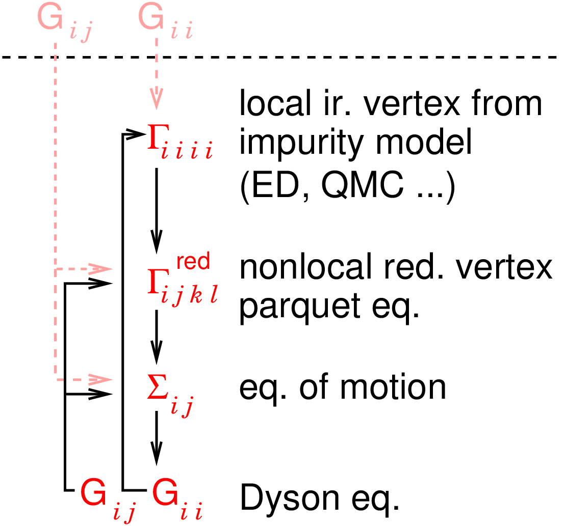
In a second step, the (non-local) reducible vertex is calculated from this (local) fully irreducible vertex. Fig. 1 shows as an example one reducible diagram constructed from the irreducible vertex. But of course, we have to sum over all reducible Feynman diagrams 22 2 That is, all Feynman diagrams, which have the local irreducble vertex and the non-local Green function as building blocks, and which do not separate into two parts when cutting two Green function lines.. This can be achieved more elegantly through the parquet equations [53, 54, 55], which is still a challenge for an actual implementation of this full DA approach.
Having the non-local reducible vertex, one can easily obtain the non-local DA self energy (third step in Fig. 3) through an exact equation which follows from the Heisenberg equation of motion [54, 55]:
| (1) |
see Fig. 4 for the diagrammatic representation. Here, , , and denote the three involved wave vectors; , , and the corresponding Matsubara frequency; the number of electrons per site, the interaction and the temperature; is the afore calculated reducible four-point vertex and the Fourier-transform of the non-local Green function taken as a starting point in the first line of Figures 3.
From the self energy Eq. (1), the dispersion relation of the lattice and the chemical potential , we can now calculate a new local and non-local Green function via the Dyson equation
| (2) |
After this fourth step of the algorithm, we can go back to step 1 and iterate the DA algorithm Fig. 3 until convergence is reached.


2.2 Restriction to the two-particle-hole channels
Instead of this full (self-consistent) DA approach, we have, in a first step, implemented a simplified scheme [44]: Neglecting the particle-particle channel of the Parquet diagrams, we restricted ourselves to the two particle-hole channels which are longitudinal and transversal, respectively, in the spin indices; see Fig. 5 b) and c). This restriction is reasonable for spin fluctuations where these channels are dominating and actually diverging close to the antiferromagnetic phase transition in two dimensions. For other physical phenomena such as superconductivity the particle-particle channel is, as a matter of course, essential.
The algorithm is shown in Fig. 6: We first calculate the irreducible vertex in the spin and charge channel from the numerically obtained susceptibility of the Anderson impurity model (step one in Fig. 6), see Eqs. (9)-(11) of Ref. \citenDGA. From this we calculate the reducible vertex (step two in Fig. 6) through the ladder summation which yields
| (3) |
where is the bubble contribution to the susceptibility.
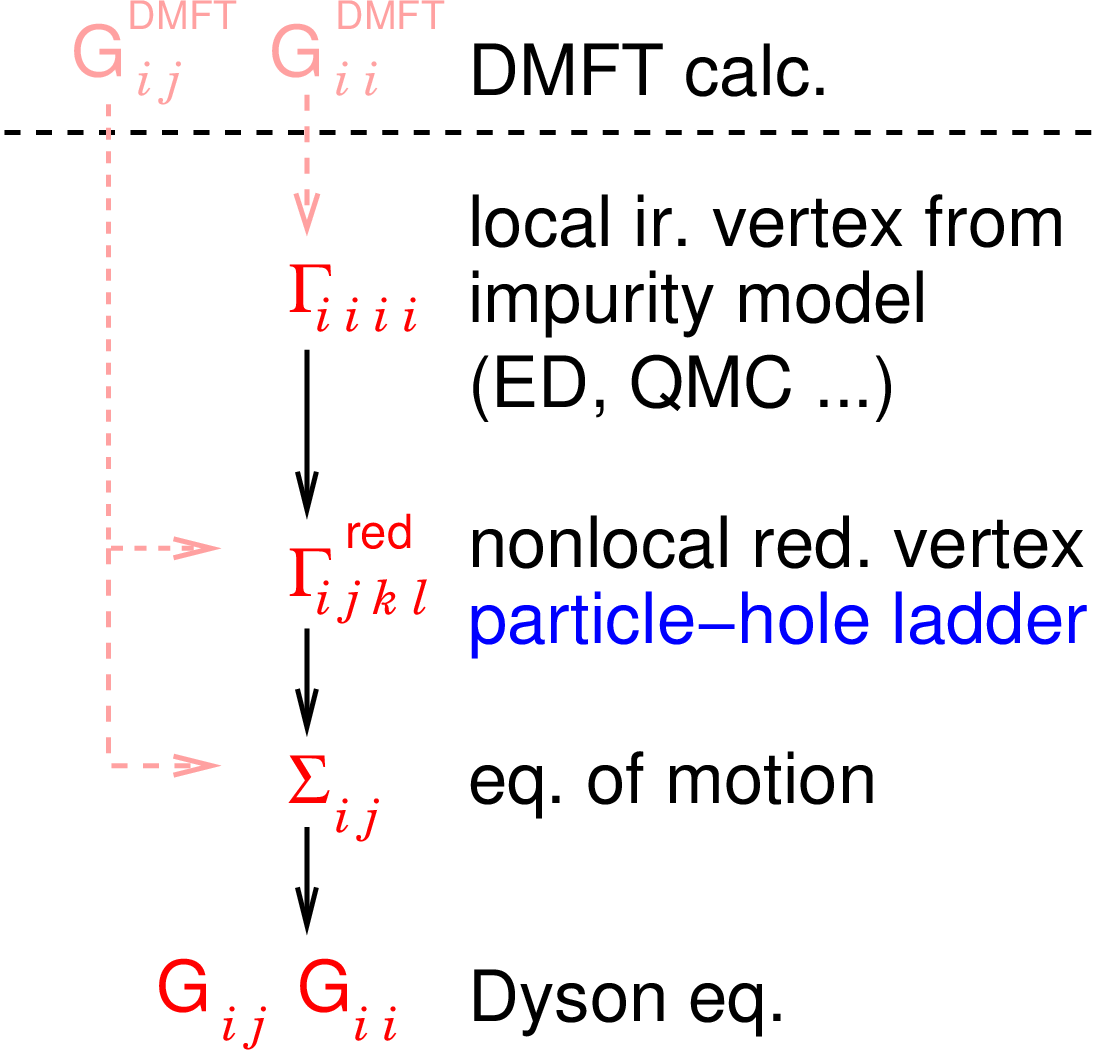
In the third step of Fig. 6, the self energy is obtained from these vertices through Eq. (1) which yields
| (4) | |||||
for the restriction to the ladder diagrams in the two particle-hole channels of Fig. 5 b) and c), respectively. Here, is the local (-summed) counterpart of . With the restriction to the two particle-hole channels, actually a non-self consistent calculation is preferable so that the algorithm ends with a calculation of the DA Green function from the self energy of Eq. (4), using the Dyson Eq. (2).
2.3 Moriyaesque correction
As a numerically inexpensive alternative to the fully self-consistent DA algorithm, we recently introduced a Moriyaeque correction [45] to the algorithm of Section 2.2. In the Moriya theory of weak itinerant magnets [56], the perturbatively obtained susceptibility is corrected as follows
| (5) |
where is the susceptibility. We do the same but for strongly correlated electron systems in the -corrected DA. In our approach, the value of is fixed by the sumrule
| (6) |
Eq. (5) translates to a correction of the vertex via
| (7) |
see Ref. \citenDGA2 for details. Hence in the DA algorithm, the correction is one additional step, the third step of Fig. 7. Otherwise the algorithm remains unchanged.
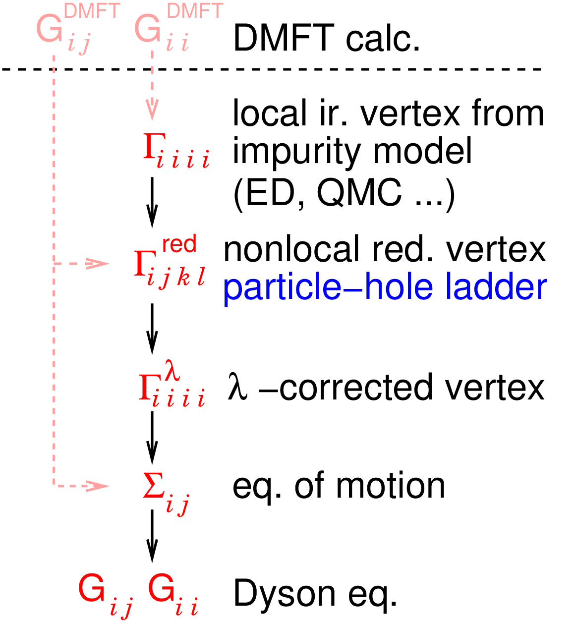
Through the correction, we include important effects of the self-consistent full DA. In particular, the reduction of the magnetic transition temperature. In two dimensions, even the Mermin-Wagner theorem is fulfilled [45].
3 Results for the Hubbard model
3.1 Three-dimensional Hubbard model
Let us turn to the results, starting with the three-dimensional Hubbard model on a cubic lattice
| (8) |
Here, denotes the hopping amplitude between nearest-neighbors, the Coulomb interaction, () creates (annihilates) an electron with spin on site , . In the following, we restrict ourselves to the paramagnetic phase with electron per site at a finite temperature . One of the cornerstones of strongly correlated electron systems for this paramagnetic phase is the Mott-Hubbard transition [57, 58], which was analyzed in DMFT in great detail [2, 3, 5] with some -by now settled- controversy for the multi-orbital case [59, 60, 61, 62, 63, 64, 65, 66, 67, 68, 69, 70, 71, 72, 73, 74, 75, 76]. What is less clear however is how far antiferromagnetic fluctuations above the ordering temperature affect the Mott-Hubbard transition. For an orientation, see the phase diagram of the Hubbard model in the left inset of Fig. 8. In DMFT, there is no feedback whatsoever of the nearby antiferromagnetic phase onto the spectrum and the self energy in the paramagnetic phase. If we, for example, completely suppress the antiferromagnetic phase through ‘‘frustrating’’ the lattice with longer-range hopping, the DMFT spectrum is the very same33 3 except for changes possibly induced by a change of the density of states due the additional hopping. DA heals this shortcoming of DMFT.

In our calculations [44], we considered three points in the paramagnetic phase of the phase diagram, marked as symbols in left inset of Fig. 8. These points are on the metallic side of the Mott-Hubbard transition and in the crossover regime where the metal continuously transforms into an insulator. In DMFT, the metallic side corresponds to a well defined quasiparticle peak (first point considered at , , where is the effective bandwidth/standard deviation of the density of states). When increasing to the crossover regime, this quasiparticle peak is first strongly damped, i.e, smeared out (second point considered at , ; for the DMFT spectrum see Fig. 9). Note, this change from a metal to a strongly damped quasi-metal was confirmed recentely by photoemssion experiments for V2O3 by Baldassarre et al. [78]. Upon a further increase of the spectrum develops a pseudogap (third point considered at , ). Or, if we take vice versa the insulating gap as a starting point, this insulating gap is filled, see Ref. \citenMo04a for an experimental validation by hands of V2O3. Increasing further, eventually a truly insulating gap is obtained.
In its main panel, Fig. 8 shows the four-point vertex irreducible in the spin channel, which was calculated numerically using exact diagonalization as an impurity solver for the Anderson impurity model [44]. As we see, the vertex strongly depends on all three frequencies (main panel and right inset). It becomes unexpectedly strong if an increasing enhances the electronic correlations. Strong local correlations result in a large vetrex which, in the vicinity of an antiferromagnetic phase transition, entail strong non-local correlations.
As discussed in Section 2.2, we can calculate the DA self energy and -resolved spectral function from the vertex of Fig. 8. The results for a wave vector on

weak damping of QP peak

QP damping strongly enhanced

more insulating
the Fermi surface are presented in Fig. 9. On the metallic side at , the non-local antiferromagnetic fluctuations lead to a relatively weak damping of the quasiparticle peak (QP). Here, the length scales, from which the main contributions of the antiferromagnetic fluctuations stem, are relatively long range. Physically, we can understand the damping simply from the fact that the quasiparticles live in a bath of bosonic spin fluctuations. The quasiparticle can scatter at these fluctuations, resulting in a reduced life time, i.e., a larger imaginary part of the self energy.
Entering the crossover regime from the metallic side, the local correlations are strongly enhanced and entail strong non-local correlations in the vicinity of the antiferromagnetic phase transition. This can be seen for in Fig. 9, where we find a strongly damped quasiparticle peak and a splitting of the Hubbard bands, which can be considered to be a precursor of the spin polaron side peaks which develop in the antiferromagnetic phase [79].
Finally, in the more insulating-like part of the crossover regime, at the antiferromagnetic correlations become even stronger, albeit they are now more short range in nature. The paramagnetic phase becomes hence considerably more insulating, indicating a shift of the Mott-Hubbard transition towards lower values of . It also shows that the Mott-Hubbard transition is strongly affected by antiferromagnetic fluctuations.
The results shown here are close to the antiferromagnetic phase transition, where the antiferromagnetic fluctuations are particularly strong. If we increase temperature, i.e., if we are deep inside the paramagnetic phase, the difference between DA and DMFT becomes very small. Already for , i.e., twice the Néel temperature, the differences are minor.
All results shown were obtained without correction; and in three dimensions the correction has only a minor (quantitative) effect. It reduces the antiferromagnetic transition temperature since is somewhat overestimated in DMFT. But the same quantitative effects as in Fig. 9 occur also with correction albeit at this lower , see Ref. \citenDGA2.
3.2 Two-dimensional Hubbard model
Let us turn now to the two-dimensional Hubbard model on a square lattice where antiferromagnetic fluctuations are expected to be much more pronounced since the particle-hole ladder diagrams diverges logarithmically in two dimensions. Our insight into these antiferromagnetic fluctuations has been recently improved not only by the cluster extensions of DMFT dealing with short-range correlations, but also by the functional renormalization group method [80, 81, 82]. The latter is very complementary to the cluster extensions since fRG deals with correlations on all length-scales, but as a (renormalized) perturbative approach it does not include the effects of strong correlations such as the Mott-Hubbard transition and strong renormalizations of the quasiparticle bands. In DA, we cover both of these aspects, strong correlations and multiple length scales, in a single approach.

Let us emphasize that in two-dimensions the Moriyaesque correction of Section 2.3 is certainly important to obtain accurate results since otherwise the antiferromagnetic fluctuations will be overestimated. Among others, the antiferromagnetic transition temperature would be, without correction, much too high, i.e., at its DMFT mean field value – instead of zero as required by the Mermin-Wagner theorem. Nonetheless, we will present here results without this correction which can be compared with the reliable -corrected results of Ref. \citenDGA2.
Figure 10 shows the same real and imaginary part of the self energy and spectral function as in the first line of Figure 9 for , but now for two-dimensions (where the effective bandwidth is ). The difference to three dimensions is dramatic since in two-dimensions the antiferromagnetic fluctuations lead to a complete redistribution of the spectrum. The quasiparticle peak of DMFT is swallowed up in a pseudogap. Even at a relatively weak interaction strength , the effects of antiferromagnetic fluctuations are much more pronounced than for a much stronger interaction strength in three dimensions. Also the -dependence is dramatic, in contrast to three dimensions, where we only showed results for one -point because of the weak -dependence. Instead, in two dimensions, the comparison of nodal [] and anti-nodal direction [] shows a strongly anisotropic pseudogap. If we would increase temperatures away from the antiferromagnetic phase transition, the pseudogap would hence first turn metallic in the nodal direction.
Fig. 11 presents results off half-filling for the asymmetric Hubbard model with in a notation where and have opposite prefactors. At weak coupling, , we clearly see a quasiparticle peak which is already somewhat damped by antiferromagnetic fluctuations; Hubbard side bands are hardly visible. Note, however the strong anisotropy of the damping which is much stronger in the anti-nodal direction.

Increasing to , the damping becomes stronger, but also more isotropic. Spectral weight is transferred to the Hubbard side bands. Upon further increasing to , these tendencies continue. The quasiparticle weight is very small; and the corresponding quasiparticle peak is strongly damped in an almost identical way for the nodal and anti-nodal direction. As we noted already for the three-dimensional Hubbard model, the antiferromagnetic fluctuations for weak coupling are very long-ranged explaining the pronounced difference between nodal and anti-nodal direction. The strong non–local correlations at larger are somewhat more short-range in nature. Consequently, the anisotropy is not so pronounced.
For comparison with angular resolved photoemission experiments, we also provide a scan through the Brillouin zone along lines of high symmetry (in the nodal and anti-nodal direction), see upper panel of Fig. 12. Note, that so that the line is connected to the (shown) line by particle-hole symmetry. When approaching the Fermi surface, the (low-energy) quasiparticle peak moves towards the Fermi energy. However, this movement stops at some point inducing a pseudogap. Let us note that with the -correction the antiferromagnetic fluctuations are weaker than without correction [46] but nonetheless still very strong. As a consequence, the pseudogap survives only in the anti-nodal direction.
Most recently, Li et al. [83] calculated also the DA lattice susceptibility. The results were obtained without -correction and are similar to those from the dual Fermion approach at higher temperatures (and much better than DMFT). However, at lower temperatures there are deviations since without correction DA overestimates antiferromagnetic fluctuations.


3.3 One-dimensional Hubbard model
One of the fascinating effects of electronic correlation is the separation of spin and charge in one dimension. Slezak et al. [46] addressed this issue in their one-dimensional DAesque calculation. As a starting point the authors considered an 8-site DCA cluster and supplemented it with additional longer range correlation as in the DA, albeit with a restriction of the vertex to the second order diagrams shown in Fig. 13.

This way, the authors where able to go to a much larger number of lattice sites than in DCA, see Fig. 14. This allowed Slezak et al. to conclude that for , spin and charge velocity are different so that an electron-like spin-charge excitation separates into its spin and charge components with time. This indicates taht the inclusion of non-local correlations results in a non-Fermi-liquid phase, suggestively a Luttinger liquid.

4 Summary and Outlook
In summary, we have presented the DA approach in an algorithmic form, including the restriction to the two particle-hole channels and the Moriyaesque -correction. Let us also emphasize here that DA is a complementary approach to the extended DMFT (EDMFT) [84, 85]. EDMFT deals with the local correlations induced by non-local interactions, whereas DA deals with the non-local correlations stemming from a local interaction. The results for the Hubbard model in , 2, and 1 dimension show effects of antiferromagnetic fluctuations such as the damping of the quasiparticle peak and the shift of the Mott-Hubbard transition to lower values of in three dimensions, the opening of a pseudo-gap and strong anisotropy of the spectrum in two-dimensions, and the spin-charge separation in one dimension.
Since short- and long-range range antiferromagnetic fluctuations are treated on the same footing with a numerical effort much more manageable than for cluster extensions of DMFT, we see excellent prospects for this approach in the future.
On a model level, a variety of fascinating phenomena can be addressed such as magnons, quantum criticality and the interplay of antiferromagnetic fluctuations and superconductivity. But also realistic multi-orbital calculations are possible for which the cluster extensions are too severely restricted because of the numerical effort. Such local density approximation (LDA) + DA calculations would, among others, allow us to study the effect of antiferromagnetic fluctuations on the Mott-Hubbard transition in V2O3 where the model scenario of Section 3.1 is realized in an actual material and which was previously studied successfully in LDA+DMFT [86, 87, 88, 89, 90]. We hope that this review, along the lines of a talk given at the Yukawa Institute in November 2007, will stimulate more groups to apply the DA approach to challenging problems of strongly correlated electron systems.
Acknowledgements
We thank the Yukawa Institute in Kyoto, Japan, for its generous hospitality and W. Metzner, M. Capone, C. Castellani, G. Sangiovanni, and R. Arita for stimulating discussions; we are indebted to M. Capone also for providing the DMFT(ED) code which has served as a starting point. This work was supported by the Russian Basic Research Foundation through Grant No. 747.2003.2 (AK).
References
- [1] W. Metzner and D. Vollhardt, Phys. Rev. Lett. 62 (1989), 324.
- [2] A. Georges and G. Kotliar, Phys. Rev. B 45 (1992), 6479.
- [3] A. Georges, G. Kotliar, W. Krauth, and M. Rozenberg, Rev. Mod. Phys. 68 13 (1996).
- [4] G. Kotliar and D. Vollhardt, Physics Today March 53 (2004).
- [5] R. Bulla, Phys. Rev. Lett. 83 (1999), 136.
- [6] M. Jarrell, Phys. Rev. Lett. 69 (1992), 168.
- [7] K. Held, M. Ulmke, N. Blümer and D. Vollhardt, Phys. Rev. B 56 (1997), 14469.
- [8] M. Ulmke, Eur. Phys. J. B 1, (1998) 301;
- [9] N. Furukawa, J. Phys. Soc. Jap. 63 (1994), 3214.
- [10] K. Held and D. Vollhardt, Euro. Phys. J. B 5 (1998).
- [11] I. A. Nekrasov, K. Held, G. Keller, D. E. Kondakov, T. Pruschke, M. Kollar, O. K. Andersen, V. I. Anisimov and D. Vollhardt, Phys. Rev. B 73, 155112 (2006).
- [12] K. Byczuk, M. Kollar, K. Held, Y.-F. Yang, I. A. Nekrasov, T. Pruschke and D. Vollhardt, Nature Physics 3 168 (2007).
- [13] A. Toschi, M. Capone, C. Castellani, and K. Held, arXiv:0712.3723.
- [14] V. I. Anisimov, A. I. Poteryaev, M. A. Korotin, A. O. Anokhin and G. Kotliar, J. Phys. Cond. Matter 9 (1997), 7359.
- [15] A. I. Lichtenstein and M. I. Katsnelson, Phys. Rev. B 57 198, 6884 (1998).
- [16] K. Held, I. A. Nekrasov, G. Keller, V. Eyert, N. Blümer, A. McMahan, R. Scalettar, T. Pruschke, V. I. Anisimov and D. Vollhardt, phys. stat. sol. (B) 243 2599 (2006).
- [17] G. Kotliar, S. Y. Savrasov, K. Haule, V. S. Oudovenko, O. Parcollet and C. A. Marianetti, Rev. Mod. Phys. 78, 865 (2006).
- [18] K. Held, Adv. Phys. 56, 829 (2007).
- [19] T. A. Maier, M. Jarrell, T. Pruschke, M. H. Hettler, Rev. Mod. Phys. 77, 1027 (2005).
- [20] G. Kotliar, S. Y. Savrasov1, G. Pálsson, and G. Biroli, Phys. Rev. Lett. 87, 186401 (2001).
- [21] A. I. Lichtenstein and M. I. Katsnelson, Phys. Rev. B 62, R9283 (2000).
- [22] M. Capone and G. Kotliar Phys. Rev. B 74, 054513 (2006).
- [23] M. H. Hettler, A. N. Tahvildar-Zadeh, M. Jarrell, T. Pruschke, and H. R. Krishnamurthy, Phys. Rev. B 58, (1998) 7475.
- [24] C. Huscroft, M. Jarrell, Th. Maier, S. Moukouri, and A. N. Tahvildarzadeh, Phys. Rev. Lett. 86, 139 (2001).
- [25] Cluster sizes can be extended by using the fluctuation exchange approximation [26] see K. Aryanpour, M. H. Hettler, and M. Jarrell, Phys. Rev. B 67, 085101 (2003).
- [26] N. E. Bickers, D. J. Scalapino, and S. R. White, Phys. Rev. Lett. 62, 961 (1989).
- [27] M. Potthoff, Eur. Phys. J. B 32 429 (2003).
- [28] M. Potthoff and M. Balzer Phys. Rev. B 75, 125112 (2007).
- [29] A. Schiller and K. Ingersent, Phys. Rev. Lett. 75 113 (1995).
- [30] G. Zaránd, D. L. Cox and A. Schiller, Phys. Rev. B 62 16227 (R) (2000).
- [31] M. Capone, M. Civelli, S. S. Kancharla, C. Castellani and G. Kotliar, Phys. Rev. B 69 195105 (2004).
- [32] E. Koch, G. Sangiovanni, and O. Gunnarsson, arXiv:0710.1247.
- [33] T. Maier, M. Jarrell, T. Pruschke and J. Keller, Phys. Rev. Lett. 85 1524 (2000).
- [34] T. A. Maier, M. Jarrell, T. C. Schulthess, P. R. C. Kent and J. B. White, Phys. Rev. Lett. 95 237001 (2005).
- [35] R. Arita and K. Held, Phys. Rev. B 73 064515 (2006).
- [36] A. I. Poteryaev, A. I. Lichtenstein and G. Kotliar, Phys. Rev. Lett. 93 086401 (2004).
- [37] V. V. Mazurenko, A. I. Lichtenstein, M. I. Katsnelson, I. Dasgupta, T. Saha-Dasgupta and V. I. Anisimov, Phys. Rev. B 66 081104 (R) (2002).
- [38] S. Biermann, A. Poteryaev, A. I. Lichtenstein and A. Georges, Phys. Rev. Lett. 94 026404 (2005).
- [39] R. Blankenbecler, D. J. Scalapino and R. L. Sugar, Phys. Rev. D 24 2278 (1981).
- [40] E. Z. Kuchinskii et al., Sov. Phys. JETP Lett. 82, 98 (2005).
- [41] M. V. Sadovskii et al., Phys. Rev. B 72, 155105 (2005).
- [42] A. N. Rubtsov, M. I. Katsnelson, and A. I. Lichtenstein, Phys. Rev. B 77, 033101 (2008)); S. Brener, H. Hafemann, A. N. Rubtsov, M. I. Katsnelson, and A. I. Lichtenstein, Phys. Rev. B 77, 195105 (2008).
- [43] V. I. Tokar and R. Monnier, cond-mat/0702011 (unpublished).
- [44] A. Toschi, A. A. Katanin, and K. Held, Phys. Rev. B 75, 045118 (2007).
- [45] A. A. Katanin, A. Toschi, and K. Held, (unpublished).
- [46] C. Slezak, M. Jarrell, Th. Maier, and J. Deisz, cond-mat/0603421 (unpublished).
- [47] H. Kusunose, J. Phys. Soc. JPN. 75, 054713 (2006).
- [48] J. E. Hirsch and R. M. Fye, Phys. Rev. Lett. 56 2521 (1986).
- [49] M. Feldbacher, K. Held and F. F. Assaad, Phys. Rev. Lett. 96 139702 (2006).
- [50] A. N. Rubtsov and A. I. Lichtenstein, JETP Lett. 80 61 (2004).
- [51] P. Werner and A. J. Millis, Phys. Rev. B 74 155107 (2006).
- [52] S. Sakai, R. Arita, K. Held and K. Aoki, Phys. Rev. B 74 155102 (2006).
- [53] Y. A. Bychkov, L. P. Gorkov, and I. E. Dzyaloshinskii, Zh. Exp. Teor. Fiz. 50, 738 (1966) [Sov. Phys. JETP 23, 489 (1966)].
- [54] N. E. Bickers and S. R. White, Phys. Rev. B 43, 8044 (1991).
- [55] V. Janiš, Phys. Rev. B 60 11345 (1999).
- [56] T. Moriya, “Spin fluctuations in Itinerant Electron Magnetism” (Springer, 1985).
- [57] N. F. Mott, Rev. Mod. Phys. 40, 677 (1968); Metal-Insulator Transitions (Taylor & Francis, London, 1990)
- [58] F. Gebhard, The Mott Metal-Insulator Transition (Springer, Berlin, 1997).
- [59] A. Liebsch, Europhys. Lett. 63 97 (2003).
- [60] A. Liebsch, Phys. Rev. Lett. 91 226401 (2003).
- [61] A. Koga, N. Kawakami, T. M. Rice and M. Sigrist, Phys. Rev. Lett. 92 216402 (2004).
- [62] A. Liebsch, Phys. Rev. B 70 165103 (2005).
- [63] A. Koga, K. Inaba and N. Kawakami, Prog. Theo. Phys. Suppl. 160 253 (2005).
- [64] A. Koga, N. Kawakami, T. M. Rice and M. Sigrist, Phys. Rev. B 72 045128 (2005).
- [65] K. Inaba, A. Koga, S. I. Suga and N. Kawakami, J. Phys. Soc. Jap. 74 2393 (2005).
- [66] K. Inaba, A. Koga, S. I. Suga and N. Kawakami, Phys. Rev. B 72 085112 (2005).
- [67] S. Biermann, L. de’ Medici and A. Georges, Phys. Rev. Lett. 95 206401 (2005).
- [68] L. de’ Medici, A. Georges and S. Biermann, Phys. Rev. B 72 205124 (2005).
- [69] R. Arita and K. Held, Phys. Rev. B 72 201102(R) (2005).
- [70] C. Knecht, N. Blümer and P. G. J. van Dongen, Phys. Rev. B 72 081103 (R) (2005).
- [71] A. Liebsch, Phys. Rev. Lett. 95 116402 (2005).
- [72] P. G. J. van Dongen, C. Knecht and N. Blümer, Phys. Stat. Sol. B 243 116 (2006).
- [73] M. Ferrero, F. Becca, M. Fabrizio and M. Capone, Phys. Rev. B 72 205126 (2005).
- [74] A. Liebsch and T. A. Costi, Euro. Phys. J. B 51, 523 (2006).
- [75] N. Blümer, C. Knecht, K. Pozgajcic and P. van Dongen (2006), cond-mat/0609758.
- [76] A. Liebsch (2006), cond-mat/0610482.
- [77] S.-K. Mo, H.-D. Kim, J. W. Allen, G.-H. Gweon, J. D. Denlinger, J.-H. Park, A. Sekiyama, A. Yamasaki, S. Suga, P. Metcalf, and K. Held, Phys. Rev. Lett. 93 076404 (2004).
- [78] L. Baldassarre, A. Perucchi, D. Nicoletti, A. Toschi, G. Sangiovanni, K. Held, M. Capone, M. Ortolani, L. Malavasi, M. Marsi, P. Metcalf, P. Postorino, and S. Lupi, Phys. Rev. B 77, 113107 (2008)
- [79] G. Sangiovanni, A. Toschi, E. Koch, K. Held, M. Capone, C. Castellani, O. Gunnarsson, S.-K. Mo, J. W. Allen, H.-D. Kim, A. Sekiyama, A. Yamasaki, S. Suga and P. Metcalf, Phys. Rev. B 73 205121 (2006).
- [80] D. Zanchi and H. J. Schulz, Phys. Rev. B 54, 9509 (1996).
- [81] C. J. Halboth and W. Metzner, Phys. Rev. Lett. 85, 5162 (2000); C. Honerkamp et al., Phys. Rev. B 63, 035109 (2001); Phys. Rev. Lett. 87, 187004 (2001).
- [82] A. A. Katanin and A. P. Kampf, Phys. Rev. B 68, 195101 (2003).
- [83] G. Li, H. Lee, and H. Monien, arXiv:0804.3043.
- [84] Q. Si and J.L. Smith, Phys. Rev. Lett. 77, 3391 (1996).
- [85] H. Kajueter, Ph.D. thesis, Rutgers University (1996).
- [86] K. Held, G. Keller, V. Eyert, V. I. Anisimov and D. Vollhardt, Phys. Rev. Lett. 86 5345 (2001).
- [87] G. Keller, K. Held, V. Eyert, D. Vollhardt and V. I. Anisimov, Phys. Rev. B 70 205116 (2004).
- [88] M. S. Laad, L. Craco and E. Müller-Hartmann, Phys. Rev. Lett. 91 156402 (2003).
- [89] M. S. Laad, L. Craco and E. Müller-Hartmann, Phys. Rev. B 73 045109 (2006).
- [90] A.I. Poteryaev, J.M. Tomczak, S. Biermann, A. Georges, A.I. Lichtenstein, A.N. Rubtsov, T. Saha-Dasgupta and O.K. Andersen, Phys. Rev. B 76, 085127 (2007).