Study of the Hubbard model on the triangular lattice using dynamical cluster approximation and dual fermion methods
Abstract
We investigate the Hubbard model on the triangular lattice at half-filling using the dynamical cluster approximation (DCA) and dual fermion (DF) methods in combination with continuous-time quantum Monte carlo (CT QMC) and semiclassical approximation (SCA) methods. We study the one-particle properties and nearest-neighbor spin correlations using the DCA method. We calculate the spectral functions using the CT QMC and SCA methods. The spectral function in the SCA and obtained by analytic continuation of the Pade approximation in CT QMC are in good agreement. We determine the metal-insulator transition (MIT) and the hysteresis associated with a first-order transition in the double occupancy and nearest-neighbor spin correlation functions as a function of temperature. As a further check, we employ the DF method and discuss the advantages and limitation of the dynamical mean field theory (DMFT), DCA and recently developed DF methods by comparing Green’s functions. We find an enhancement of antiferromagnetic (AF) correlations and provide evidence for magnetically ordered phases by calculating the spin susceptibility.
pacs
71.10.FdI Introduction
The physics of systems which exhibit strong electronic correlations and geometric frustration at the same time is still unclear and therefore interesting. Recent experiments, such as discovery of the pyrochlore compound [1] which show heavy fermion behavior and organic materials -(BEDT-TTF)2X [2] which exhibit various interesting phases, motivated us to study the frustrated systems in more detail. Theoretically they are described by a two-dimensional one-band Hubbard or t-J models on the triangular lattice. It is well known that on the square lattice at half-filling the ground state is a Mott insulator with AF order but on the triangular lattice the frustration suppresses AF order and we expect to find a Mott transition.
In this paper, we study the model which was presented in a recent paper of Imai and Kawakami [3]. They used the DCA method [17, 18] in combination with noncrossing approximation (NCA) and fluctuation exchange (FLEX) methods at high temperature regions in metallic states to demonstrate how geometrical frustration suppresses AF correlations by tuning aniotropic hopping t’ in Fig. 1(a). However, the methods used in the paper are limited to high temperatures. For this reason we investigate the low temperature MIT with a first-order transition and the evidence of magnetically ordered phases. In addition, we test the newly developed DF method [14, 15, 16] beyond the single-site DMFT method by comparing the Green’s function of single-site DMFT [4, 5], DF and DCA methods with =4 and =16.
The paper is organized as follows: In Sec. II, we introduce the model and discuss the advantages and limitations of the computational methods briefly. In Sec. III, we present the results. In the first part, we compare the spectral functions which exhibit the quasiparticle peak and gap structure obtained by the SCA [20, 21] and CT QMC [19] methods with Pade approximation. In the second part, we show that the MIT is a first-order transition by measuring the total density of state (DOS), double occupancy and nearest-neighbor spin correlations. In the third part, we calculate the single-particle Green’s function using the DMFT, DF and DCA methods with =4 and =16. Specifically, we show that the DF method which is based on the single-site DMFT method can describe non-local correlation effects very well. In the last part, we explore the spin susceptibility using the DF method. Sec IV, we give a summary work.
II Model and Methods
II.1 Model
We consider the two-dimensional Hubbard model on the triangular lattice.
| (1) |
where is the annihilation (creation) operator of an electron with spin at the -th site, t is the hopping matrix element and represents the Coulomb repulsion. In this paper we only consider the isotropic hopping of t’=t in Fig. 1(a)-(b).

Due to the geometrical frustration, this model has broken particle-hole symmetry even at half-filling unlike the case of the square lattice and the original Brillouin zone (BZ) has an hexagonal structure shown by the doted line in Fig. 1(c). For this model there are a lot of studies using a variety of methods such as the path integral renormalization group method [6], the quantum Monte carlo method [7], the DMFT [8, 9] and the cluster extension method of DMFT [10, 11, 12, 13]. Especially, DF [14, 15, 16] and DCA methods [17, 18] are noteworthy because both methods can capture non-local correlation effect which are lost in the single-site DMFT and they are computational cheaper and have less of a sign problem than the lattice QMC calculation. In short, DCA method can treat correlations up to a cluster size accurately and long range correlations are considered on the mean-field level. On the other hand, the DF method considers long range as well as short range correlations within pertubative diagram expansion, which is done by introducing an auxiliary field. Because each method has its limitations, it is useful to compare results of both. We use the CT QMC method [19], which can access the low temperature region easily without the Trotter error, as well as the SCA method [20, 21] as impurity solvers.
II.2 DCA method
The DCA method [17, 18] assumes that the self-energy in the first BZ is constant and the coarse-grained Green’s function (DCA equation) is given by Eq. (2).
| (2) |
where N is the number of lattice sites in each first BZ and the summation over is calculated in each of them. For delimitation we consider an example of =4 in order to explain the DCA method. The first BZ (dashed line in Fig. 1(c)) is created by partitioning the original BZ. Like the standard procedure of DMFT, the coarse-grained Green’s function is determined self-consistently after several iterations. The main advantages of the DCA method are that it considers short range correlations in the cluster size exactly and has smaller computational load and fermionic sign problem compared to the lattice calculation by QMC method. However, it is still expensive in terms of computational time and long range correlations are just treated on the mean-field level.
II.3 DF method
The DF method [14, 15, 16] is a relatively new method which can describe non-local correlations based on the single-site DMFT method. The basic idea of the DF method is to convert the hopping of different fermions into an effective coupling to an auxiliary field. Each lattice site can be viewed as an impurity which is easily described by the DMFT method. While these impurities are not totally isolated, they are perturbatively coupled by the auxiliary field. The starting point is the action of DMFT which is represented in the form
| (3) |
where is the hybridization function describing the interaction of an effective impurity with a bath and is the fermionic Matsubara frequency. Here we use the dispersion relation based on the correspondence of a triangular lattice to a square lattice with diagonal hopping (b) in Fig. 1. This “square lattice” has a simple BZ which makes the momentum summation to be easily performed by using the fast Fourier transformation (FFT). By the dual transfomation, the lattice problem is changed to an impurity problem which is coupled by the auxiliary field .
| (4) | |||||
The lattice Green’s function is derived from the exact relation between Eq. (3) and Eq. (4).
| (5) |
where is the dual Green’s function and is the local Green’s function calculated by single-site DMFT. The main point for this method is that in Eq. (4) the integration over and c can be performed separately for each site which yields an effective action of the auxiliary field and . The Taylor expansion in powers of and will introduce the two, three, ,-particle vertex functions. Using the skeleton-diagram expansion we calculate the dual self-energy and dual Green’s function by the Dyson equation. We obtain the lattice Green’s function via Eq. (5). Even though the DF method is an approximate method, it considers not only the short range but also the long range correlations. Moreover, the calculation of the two-particle properties does not introduce serious computational burden and fermionic sign problem.
II.4 SCA method
At high temperature the Monte carlo integration over the auxillary classical field can be approximated by assuming const. This approximation is useful because it allows to check the QMC results at temperature quickly. In this part we introduce the SCA method [20, 21] as impruity solver for DCA method. We consider a four-site cluster(=4) for triangular lattice like the structure of Fig. 1(a). In this case the partition function is defined as a functional integral over 24-component spin and site-dependent spinor fields and c as
| (6) |
where
| (7) |
Here is the Weiss field which is determined self-consistently by Eq. (2) and =1/T is the inverse temperature. In this model is given as
We can decouple the interaction term as
| (8) |
with . We employ the continuous Hubbard-Stratonovich(HS) transformation in order to decouple M terms related to auxiliary field . Here we assume that is independent and N term is neglected because charge fluctuations are small at half-filling. By a Grassmann integration we can rewrite the partition function which is represented as a four-dimensional integration in terms of and the fermionic Matsubara frequency.
| (9) |
where the effective action is defined by
| (10) |
where is defined as
| (11) |
Here j=1,2,3,4 and is the z-component Pauli matrix. The impurity Green’s function is calculated by
| (12) |
In real frequency space the spectral function is calculated by replacing to . The SCA method is not only cheap in computational time but also gives good results in the strong coupling regime. On the other hand, it underestimates the spectral function around and gives qualitatively wrong results at low temperature.
II.5 CT QMC method
Here we describe the CT QMC method [19]. The starting point is action can be split into an unperturbed action and an interaction part W. By Taylor expansion of partition function in powers of the interaction U, we can reexpress the partition function
| (13) |
with the correlation function.
| (14) |
where is the partition function for unperturbed system, integration over implies the integral over and sum over all lattices states and is the time-ordering operator. By Wick’s theorem the weight function is determined by
| (15) |
where is the bare Green’s function. The Green’s function is defined by
| (16) |
and by the fast-update formula [19, 22] and the Fourier transformation we can rewrite the Green’s function in the Matsubara frequencies space.
| (17) |
where and is the bare Green’s function. A two-particle Green’s function related to a vertex function for DF method can be calculated by Wick’s theorem. With this method it is possible to perform calculations in low temperature regions which cannot be accessed easily with determinant QMC method without Trotter error. For example, the matrix size of the CT QMC method is scaled by k which is comparable to determinant QMC [23] method scaled by k . Moreover, even if the recently developed strong-coupling CT QMC method, [24, 22] which is based on a diagrammatic expansion in the impurity-bath hybridization, has nice advantages such as removing the fermionic sign problem and calculating lower temperature regions, its computational effort in large cluster is increased exponentially by the number of sites . However, our CT QMC method can overcome the problem because the computational burden only increases linealy with the number of sites.
III RESULTS
III.1 Comparison of the spectral functions for the SCA and C-T QMC methods
First we compare the one-particle spectral functions obtained from the SCA and CT QMC methods with Pade approximation for analytical continuation. Since the process, in which calculated by the CT QMC method changes into with Pade approximation, introduces large error, it is useful check to compare QMC results to SCA results which are calculated in real frequency space. Moreover, because the systems with geometrical frustration have large , the SCA method is suitable for this model. The spectral function is given by
| (18) |
We compare the Green’s function on the Fermi surface K=. The results are shown in Fig. 2(a)-(b). At U=6 in Fig. 2(a) the difference of both results is that the peak of quasiparticle obtained from QMC method lies around the Fermi level(=0) due to the geometrical frustration. On the other hand, the peak obtained from SCA method deviates from the Fermi level because the SCA underestimates the =0 peak. At U=9 in Fig. 2(b) the agreement of both results is more reasonable and a (pseudo)gap structure is represented.

III.2 The metal-insulator transition with a first-order transition
Here we present our results on the MIT due to geometrical frustration effect obtained with the CT QMC method. In previous study of unfrustrated square lattice using DCA method, it was shown that short-range AF correlations destroy the Fermi liquid quasiparticle peak at finite temperature [25]. According to Ref. 25, the authors increased the system size gradually in the weak-coupling regime on unfrustrated square lattice and measured the total DOS. Eventually, even if the quasiparticle peak is clearly visible at =1 in DMFT method, there is a small gap at =16 which completely disappears at =64. In this system we did not find a band insulator transition. However, on the triangular lattice the frustration is enough to destroy the AF correlation. In Fig. 3(a)-(b), we can see the MIT by comparing the total DOS for U=6, U=10 and =4 using the DCA method with =4 and =16. Unlike the results for unfrustrated square lattice, the quasiparticle peak around the Fermi level is clearly seen with increasing at U=6 in Fig. 3(a). At U=10 in Fig. 3(b) we can see the Mott insulator in both =4 and =16. This is evidence of a MIT on the triangular lattice.

In the low temperature regime we are also interested in finding whether there is a first-order transition or a continuous transition and how the geometrical frustration effects the system. We expect our system to have a first-order transition because of the recent two cellular DMFT (CDMFT) results [26, 12] which show a first-order transition on the square lattice with =4 and on the triangular lattice with anisotropic hoping at low temperatures. In order to find evidence of a first-order transition we measure the double occupancy at several temperatures. Our result is shown in Fig 4. The system displays a crossover between metal and insulator at T=0.2. At T=0.1 we can see hysteresis associated with a first-order transition and at lower temperature hysteresis is more clear.

In order to understand the system more clearly we calculate the nearest-neighbor spin correlation function which is shown in Fig. 5. At jumps of the spin correlation function indicate the MIT arising from competetion between the quasiparticle formation and the frustrated spin correlation. Specifically, the spin correlation is enhanced weakly at =7.2 for T=0.2 while it is increased rapidly at in T 0.1. Here is =6.9 for T=0.1 and =6.7 for T=0.05. This means that the entropy at T=0.2 and in T 0.1 is released by geometrical frustration and spin correlation, respectively as temperature decreases and the entropy at insulator state in T 0.1 has small value which is triggered a first-order transition because of a formation of AF state.

Moreover, we find that the anomalous character in the metallic state is unlike the results of the nearest-neighbor spin correlation on the Kagome lattice[27]. In the metallic state the spin correlation is weak. This is the reason that geometrical frustration is more dominant than AF spin correlation at lower temperature in the metallic state because the frustration on the triangular lattice is stronger than that on the Kagome lattice. However, in the insulating state AF spin correlation is enhanced stronger than the frustration effect at lower temperature so the spin correlation is strong with decreasing temperature.
III.3 Comparison of Green’s functions among the DCA, DF and DMFT methods
In this part we using the DMFT, DF and DCA methods with =4 and =16 to study the non-local correlation effects and compare the on-site and nearest-neighbor Green’s functions in the Matsubara space.
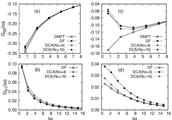
In Fig. 6(a)-(d), we present the Green’s functions obtained from DMFT, DF and DCA method with =4 and =16 for =4, U=6 and U=10. The on-site Green’s function of DMFT method in Fig. 6(a) is similiar to the results of DCA and DF method and all of these indicate the metallic states. A remarkable point is that in Fig. 6(a) and (b), both the on-site and nearest-neighbor Green’s functions obtained from DF method are closer to those of the DCA method with =16 than =4. In Fig. 6(c) at U=10 the on-site Green’s function calculated by the DMFT still shows the metallic state which overestimates the value of because of a lack of non-local correlation. However, the DCA and DF methods can capture the insulating state and the agreement of the on-site Green’s function calculated by the DF and DCA methods with =16 is quite reasonable. In Fig. 6(d), the nearest-neighbor Green’s functions obtained from DF method are still closer to those of =16 than =4. This suggests that despite the fact that the DF method is a perturbative method, it would describe physics quite well than the DCA method with small cluster size. We expect that considering high-order diagrams will improve the results of the DF method.
III.4 The spin susceptibility using the DF method
In order to explore a magnetic instability we measure the spin susceptibility using the DF method. The reason why we employ DF method for the spin susceptibility is that the cluster-extension method of the DMFT takes a large amount of time in order to obtain the two-particle properties. On the other hand, because the DF method includes the vertex renormalization through the Bethe-Salpeter equation, the computational burden is not serious and the results are relatively good compared to those of QMC method [16]. Fig. 7(a) shows for U/t=10.0 and where the system is in the insulating state. The has a maximum peak at . The spin susceptibility at and q=(0,0) as a function of temperature is exhibited in Fig. 7(b). As temperature decreases, at shows strong enhancement of the AF correlations.

IV CONCLUSIONS
In summary, we have investigated the Hubbard model on the triangular lattice using the DCA and DF method. Using the DCA method we compared the spectral functions obtained from SCA and CT QMC methods. We found a good agreement of both methods and the quasiparticle peak and gap structure are presented in the weak and the strong coupling regions, respectively. We found a MIT with a first-order transition at low temperatures because of the effect of geometrical frustration. Moreover, we employed the DF method which considers the long range as well as short range correlations and compared the Green’s functions of the DF method to those of the DMFT and DCA method with =4 and =16. We found that the DF method does not only overcome the overestimation of in DMFT method but also that its results are closer the case of =16 than =4. Finally, we calculated the spin susceptibility via DF method. We found that the at grows rapidly as temperature decreases.
We would like to thank A. Lichtenstein and E. Gorelov for their assistance in implementing the CT QMC code.
References
- [1] K. S. et al, Phys. Rev. Lett. 78, 3729 (1997).
- [2] R. Mckenzie, Science 278, 820 (1997).
- [3] Y. Imai and N. Kawakami, Phys. Rev. B 65, 233103 (2002).
- [4] A. Georges, G. Kotliar, W. Krauth, and M. Rozenberg, Rev. Mod. Phys. 68, 13 (1996).
- [5] W. Metzner and D. Vollhardt, Phys. Rev. Lett. 62, 324 (1989).
- [6] H. M. et al, J. Phys. Soc. Jpn 71, 2109 (2002).
- [7] N. Bulut, W. Koshibae, and S. Maekawa, Phys. Rev. Lett 95, 037001 (2005).
- [8] K. Aryanpour, W. Pickett, and R. Scalettar, Rev. Rev. B 74, 085117 (2006).
- [9] J. Merino, M. D. M. Dumm, N. Drichko, and R. H. Mckenzie, Phys. Rev. Lett. 100, 086404 (2008).
- [10] O. Parcollet, G. Biroli, and G. Kotliar, Rev. Rev. Lett 92, 226402 (2004).
- [11] B. Kyung, Phys. Rev. B 75, 033102 (2007).
- [12] T. Ohashi, T. Momoi, H. Tsunetsugu, and N. Kawakami, Phys. Rev. Lett. 100, 076402 (2008).
- [13] B. Kyung and A.-M. Tremblay, Phys. Rev. Lett. 97, 046402 (2006).
- [14] A. Rubtsov, M. Katsnelson, and A. Lichtenstein, Phys. Rev. B 77, 033101 (2008).
- [15] S. Brener, H. Hafermann, A. Rubtsov, M. Katsnelson, and A. Lichtenstein, Phys. Rev. B 77, 195105 (2008).
- [16] G. Li, H. Lee, and H. Monien, eprint cond-mat/08043043.
- [17] M. Hettler, A. Tahrildar-zadeh, M. Jarrell, T. Pruschken, and H. Krishnamurthy, Phys. Rev. B 58, R7475 (1998).
- [18] M. Hettler, M. Mukherjee, M. Jarrell, and H. Krishnamurthy, Phys. Rev. B 61, 12739 (2000).
- [19] A. Rubtsov, V. Savkin, and A. Lichtenstein, Phys. Rev. B 72, 035122 (2005).
- [20] S. Okamoto, A. Fuhrmann, A. Comanac, and A. Millis, Phys. Rev. B 71, 235113 (2005).
- [21] A. Fuhrmann, S. Okamoto, H. Monien, and A. J. Millis, Phys. Rev. B 75, 205118 (2007).
- [22] K. Haule and G. Kotliar, Phys. Rev. B 75, 155113 (2007).
- [23] J. Hirsch and R. Fye, Phys. Rev. Lett. 56, 2521 (1986).
- [24] P.Werner, A.Commanac, L. D. Medici, M. Troyer, and A. Millis, Phys. Rev. Lett. 97, 076405 (2006).
- [25] S. Moukouri and M. Jarrell, Phys. Rev. Lett. 87, 167010 (2001).
- [26] H. Park, K. Haule, and G. Kotliar, eprint cond-mat/08031324.
- [27] T. Ohashi, N. Kawakami, and H. Tsunetsugu, Phys. Rev. Lett. 97, 066401 (2006).