\runtitle2-column format camera-ready paper in LaTeX \runauthorK.G. Chetyrkin
SFB/CPP-08-47
TTP08-27
BNL-HET-08/16
New Results in Four and Five Loop
QED calculations
Thanks:
Talk presented at 9th DESY Workshop on Elementary Particle Theory:
Loops and Legs in Quantum Field Theory, Sondershausen, Germany, 20-25 April 2008.
Abstract
We report on two recent multiloop results in QED: (i) the four-loop corrections to the conversion relations between the QED charge renormalized in the on-shell and schemes; (ii) analytical evaluation of a class of asymptotic contributions to the muon anomaly at five-loops.
1 Introduction
The study of the anomalous magnetic moment of the muon is a long-standing challenge for both theory and experiment. It has been measured with impressive accuracy at the level of 0.5 parts per million [1]: . From theory side the anomalous magnetic moment has been studied in great detail through the computation of higher order corrections (see, e.g. reviews [2, 3, 4]). These higher order corrections to are basically classified into three classes: pure QED, electroweak and hadronic contribution.
A discussion of the electroweak and hadronic corrections can be found in Ref. [5] and references therein. Within this work we consider higher order corrections to the pure QED part. Starting from two-loop, diagrams with internal fermion-loops can arise, where the fermion-type of the internal loop can in general be different from the external muon. The one-loop [6] and two-loop [7, 8, 9, 10, 11, 12, 13] contributions have been computed more than 50 years ago. The three-loop order has been computed numerically and analytically [14, 15, 16, 17, 18, 19, 20]
The complete calculation of hundreds of diagrams contributing to the muon anomaly at four loop order is only possible by numerical integration, which was performed in a remarkable long-term effort by Kinoshita and his collaborators [21, 22]. Even some numerically important five-loop diagrams have been computed by now [23].
Accurate numerical calculation of highly divergent multiloop Feynman amplitudes is highly nontrivial task. The analytical calculation (of even a very particular class of diagrams) should be quite useful as an independent check in both directions! (see e.g. instructive examples in Refs. [24, 25, 26, 27, 21, 28, 29]).
In particular starting from two-loop there arise logarithmic contributions of the type , where is the mass of the muon and the mass of the electron, respectively. In view of the large mass ratio one can expect, that these logarithms play a dominant role. The logarithmically enhanced contributions arise from the insertion of the electron vacuum polarization (eVP) into the first order muon vertex diagram, but they can also appear through light-by-light (LBL) scattering diagrams. Examples for both diagram types are shown in Fig. 1.
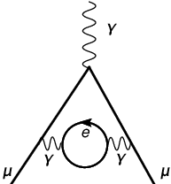
eVP
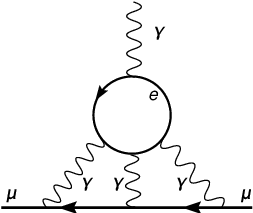
LBL
In what follows we will consider only eVP contributions to which are produced from diagrams like Fig 1 (eVP) but with the photon propagator receiving all possible QED perturbative corrections made of electron loops and photon exchanges only. The general structure of eVP was throughly studied long ago in the pioneering publications of B. Lautrup and E. De Rafael and R. Barbieri and E. Remiddi [30, 31].
There it was found, that the asymptotic part of the muon anomaly , which contains these logarithmic contributions originating form the electron vacuum polarization function insertions and the mass independent term, can be obtained with the help of the electron vacuum polarization function in the asymptotic limit . The corresponding master formula reads
| (1) |
Here
| (2) | |||
| (3) |
In the above formulas is the photon polarization operator (in QED incorporating exactly one fermion field), is the on-shell fermion mass, and the fine structure constant is defined in the classical OS-scheme by the condition:
| (4) |
Once is computed to some order in the master formula (1) immediately delivers the corresponding eVP contribution to .
At present this technique has been applied in order to find the complete eVP contributions to up to three-loop and four-loop order [30, 31, 25, 27].
In our talk we extend these results by one order. As a by-product we will also derive the four-loop corrections to the conversion relations between the QED charge renormalized in the on-shell and schemes.
2 Photon polarization operator in -scheme
Thus, the main problem is to compute the asymptotic photon polarization operator ()
with every being, in fact11 1 This is a consequence of the Weinberg theorem [32]., a polynomial of order not higher than in .
It is very useful to consider first the photon polarization operator in -scheme written as where and are the running coupling constant and the fermion mass in the -scheme, while stands for the renormalization point. Indeed, the polarization function has a smooth massless limit:
| (5) |
A use of the fundamental concept of the invariant charge [33, 34] directly leads to the connection between and
| (6) |
Eq. (6) allows one (see e.g. [30]) to relate and through the polarization operator at zero momentum transfer
| (7) |
Thus, to compute the at four loops we need to know the polarization function in the massless and momentum-less limits as well as the relation between on-shell and masses of a fermion in QED at three loops. The latter, fortunately, is available from [35, 36].
2.1 Massless limit of
2.2 Momentum-less limit of
The limit leads to the evaluation of massive tadpole diagrams. Their computation has been performed with FORM [37, 42, 43] based programs. All appearing tadpole diagrams have been reduced to master integrals with the help of Laporta’s algorithm [20, 44]. The arising polynomials in the space-time dimension have been simplified with the program FERMAT [45]. The remaining master integrals are known analytically to sufficient high order in and have been taken from Refs. [46, 47, 48, 49, 50, 51, 52, 53, 54]. The following result for at was found
| (9) | |||||
Here , is Riemann’s zeta function and .
3 Conversion formulas for
4 Asymptotic photon polarization operator in on-shell scheme
The combined use of eqs. (8,9,11) immediately leads us to the the following expression for the four-loop contribution to the asymptotic photon polarization22 2 All terms proportional to in (12) could be derived in easy way from renormalization group arguments as explained in [30]. In addition, the process of constructing one should invert the power series for , which also produces remarkably easy-to-compute factorizable fourth order contributions to like and so on (see e.g. [56] and references therein). However, to include power suppressed terms of order to is much less trivial even for the factorizable contributions [57, 58].
| (12) | |||||
Note that in the process of deriving (12) one needs also and for . We have not write the corresponding results explicitly to save space; the reader could find them e.g. in Ref. [27].
5 eVP contribution to the muon anomaly at fifth order
Combining eqs. (1,12) we arrive to our main result: the complete eVP contribution to the muon anomaly at order (below we write down only the new five-loop result; we have confirmed all previously known eVP contributions to at three and four loops)
| (13) |
| (14) | |||||
where . Finally, numerically, the result reads:
| (15) |
Eq. (15) also displays the decomposition of the full result into two pieces, corresponding to non-singlet and singlet contributions to the photon polarization operator (see, e.g. [59]).
6 Conclusion and Acknowledgment
We hope that our main result (15) for the complete fifth order eVP contribution to the muon anomaly could be of some use for testing the complicated numerical simulations like it happened a few times in the past.
We are grateful to J.H. Kühn for his interest in the work and careful reading the manuscript.
This work was supported by the Deutsche Forschungsgemeinschaft in the Sonderforschungsbereich/Transregio SFB/TR-9 “Computational Particle Physics”, by INTAS (grant 03-51-4007) and by RFBR (grant 08-02-01451). This work was also partially supported by U.S. Department of Energy under contract No.DE-AC02-98CH10886. The computer calculations were partially performed on the HP XC4000 super computer of the federal state Baden-Württemberg at the High Performance Computing Center Stuttgart (HLRS) under the grant “ParFORM”.
Note added. Very recently, two months after the conference, the result for the five-loop eVP contribution to the muon anomaly from singlet diagrams have been published by T. Aoyama, M. Hayakawa, T. Kinoshita, M. Nio and N. Watanabe [60]. Their result reads:
| (16) |
One observes a good agreement for the singlet case between the numerical result (16) and our prediction (15). The remaining 2.6 % difference presumably comes from power suppressed corrections to the asymptotic result.
References
- [1] Muon G-2, G.W. Bennett et al., Phys. Rev. D73 (2006) 072003, hep-ex/0602035.
- [2] K. Melnikov and A. Vainshtein, Theory of the muon anomalous magnetic moment, Berlin, Germany: Springer (2006) 176 p.
- [3] F. Jegerlehner, Acta Phys. Polon. B38 (2007) 3021, hep-ph/0703125.
- [4] J.P. Miller, E. de Rafael and B.L. Roberts, Rept. Prog. Phys. 70 (2007) 795, hep-ph/0703049.
- [5] W.M. Yao, J. Phys. G 33 (2007) 1, and 2007 partial update for the 2008 edition.
- [6] J.S. Schwinger, Phys. Rev. 82 (1951) 664.
- [7] R. Karplus and N.M. Kroll, Phys. Rev. 77 (1950) 536.
- [8] A. Petermann, Helv. Phys. Acta 30 (1957) 407.
- [9] C.M. Sommerfield, Phys. Rev. 107 (1957) 328.
- [10] H. Suura and E.H. Wichmann, Phys. Rev. 105 (1957) 1930.
- [11] A. Petermann, Phys. Rev. 105 (1957) 1931.
- [12] H.H. Elend, Phys. Lett. 20 (1966) 682.
- [13] W.G. Erickson and H.T. Liu, UCD-CNL-81 report (1968) .
- [14] T. Kinoshita, Phys. Rev. Lett. 75 (1995) 4728.
- [15] S. Laporta and E. Remiddi, Phys. Lett. B265 (1991) 182.
- [16] S. Laporta and E. Remiddi, Phys. Lett. B301 (1993) 440.
- [17] S. Laporta, Phys. Rev. D47 (1993) 4793.
- [18] S. Laporta, Phys. Lett. B343 (1995) 421, hep-ph/9410248.
- [19] S. Laporta and E. Remiddi, Phys. Lett. B356 (1995) 390.
- [20] S. Laporta and E. Remiddi, Phys. Lett. B379 (1996) 283, hep-ph/9602417.
- [21] T. Kinoshita and M. Nio, Phys. Rev. D70 (2004) 113001, hep-ph/0402206.
- [22] T. Kinoshita and M. Nio, Phys. Rev. D73 (2006) 053007, hep-ph/0512330.
- [23] M. Nio et al., Nucl. Phys. Proc. Suppl. 169 (2007) 238.
- [24] R.N. Faustov et al., Phys. Lett. B254 (1991) 241.
- [25] T. Kinoshita, H. Kawai and Y. Okamoto, Phys. Lett. B254 (1991) 235.
- [26] T. Kinoshita, B. Nizic and Y. Okamoto, Phys. Rev. D41 (1990) 593.
- [27] D.J. Broadhurst, A.L. Kataev and O.V. Tarasov, Phys. Lett. B298 (1993) 445, hep-ph/9210255.
- [28] P.A. Baikov and D.J. Broadhurst, (1995), hep-ph/9504398.
- [29] T. Kinoshita and M. Nio, Phys. Rev. D73 (2006) 013003, hep-ph/0507249.
- [30] B. Lautrup and E. De Rafael, Nucl. Phys. B70 (1974) 317.
- [31] R. Barbieri and E. Remiddi, Nucl. Phys. B90 (1975) 233.
- [32] S. Weinberg, Phys. Rev. 118 (1960) 838.
- [33] N.N. Bogolyubov and D.V. Shirkov, Nuovo Cim. 3 (1956) 845.
- [34] D.V. Shirkov, (1998), hep-th/9903073.
- [35] K.G. Chetyrkin and M. Steinhauser, Nucl. Phys. B573 (2000) 617, hep-ph/9911434.
- [36] K. Melnikov and T.v. Ritbergen, Phys. Lett. B482 (2000) 99, hep-ph/9912391.
- [37] J.A.M. Vermaseren, New features of FORM, math-ph/0010025 (2000) , math-ph/0010025.
- [38] D. Fliegner, A. Retey and J.A.M. Vermaseren, (1999), hep-ph/9906426.
- [39] D. Fliegner, A. Retey and J.A.M. Vermaseren, (2000), hep-ph/0007221.
- [40] P. Nogueira, J. Comput. Phys. 105 (1993) 279.
- [41] P.A. Baikov, Phys. Lett. B385 (1996) 404, hep-ph/9603267.
- [42] J.A.M. Vermaseren, Nucl. Phys. Proc. Suppl. 116 (2003) 343, hep-ph/0211297.
- [43] M. Tentyukov and J.A.M. Vermaseren, Comput. Phys. Commun. 176 (2007) 385, cs/0604052.
- [44] S. Laporta, Int. J. Mod. Phys. A15 (2000) 5087, hep-ph/0102033.
- [45] R.H. Lewis, Fermat’s User Guide, http://www.bway.net/˜lewis/ .
- [46] S. Laporta, Phys. Lett. B549 (2002) 115, hep-ph/0210336.
- [47] K.G. Chetyrkin et al., Eur. Phys. J. C40 (2005) 361, hep-ph/0412055.
- [48] B.A. Kniehl and A.V. Kotikov, Phys. Lett. B638 (2006) 531, hep-ph/0508238.
- [49] Y. Schröder and A. Vuorinen, JHEP 06 (2005) 051, hep-ph/0503209.
- [50] Y. Schröder and M. Steinhauser, Phys. Lett. B622 (2005) 124, hep-ph/0504055.
- [51] K.G. Chetyrkin et al., Nucl. Phys. B742 (2006) 208, hep-ph/0601165.
- [52] E. Bejdakic and Y. Schröder, Nucl. Phys. Proc. Suppl. 160 (2006) 155, hep-ph/0607006.
- [53] B.A. Kniehl and A.V. Kotikov, Phys. Lett. B642 (2006) 68, hep-ph/0607201.
- [54] B.A. Kniehl et al., Phys. Rev. Lett. 97 (2006) 042001, hep-ph/0607202.
- [55] D.J. Broadhurst, Z. Phys. C54 (1992) 599.
- [56] A.L. Kataev, hep-ph/0602098 (2006), hep-ph/0602098.
- [57] A. Czarnecki and M. Skrzypek, Phys. Lett. B449 (1999) 354, hep-ph/9812394.
- [58] J.P. Aguilar, D. Greynat and E. De Rafael, Phys. Rev. D77 (2008) 093010, 0802.2618.
- [59] K.G. Chetyrkin, J.H. Kühn and A. Kwiatkowski, Phys. Rep. 277 (1996) 189.
- [60] T. Aoyama et al., (2008), hep-ph/0806.3390.