First study of the three-gluon static potential in Lattice QCD
Abstract
We estimate the potential energy for a system of three static gluons in Lattice QCD. This is relevant for the different models of three-body glueballs have been proposed in the literature, either for gluons with a constituent mass, or for massless ones. A Wilson loop adequate to the static hybrid three-body system is developed. We study different spacial geometries, to compare the starfish model with the triangle model, for the three-gluon potential. We also study two different colour structures, symmetric and antisymmetric, and compare the respective static potentials. A first simulation is performed in a periodic Lattice, with and fm.
I Introduction
We explore, in Lattice QCD, the static potential of the three-body glueball system composed of three gluons, using Wilson loops. The interest in three-body gluon-gluon-gluon systems is increasing in anticipation to the future experiments BESIII at IHEP in Beijin, GLUEX at JLab and PANDA at GSI in Darmstadt, dedicated to study the mass range of charmonium, with a focus in its plausible hybrid excitations. Even before the glueballs are discovered, the study of two-gluon and three–gluon glueballs are respectively relevant to the pomeron [1, 2] and to the odderon [3]. Thus several models of three-gluon models have already started to be developed [3, 4, 5, 6, 8, 7].
The relevance of computing the static potentials in Lattice QCD for 3-gluon models is partly motivated by the plausible existence of a constituent mass for the gluon. Several evidences of a gluon effective mass of 600-1000 MeV, much larger than , exist from the Lattice QCD gluon propagator in Landau gauge, [9, 10], from Schwinger-Dyson and Bogoliubov-Valatin solutions for the gluon propagator in Landau gauge [11], from the analogy of confinement in QCD to supercondutivity [12], from the Lattice QCD breaking of the adjoint string [13], from the Lattice QCD gluonic excitations of the fundamental string [14] from constituent gluon models [4, 15, 16] compatible with the Lattice QCD glueball spectra [17, 18, 19, 20], and with the Pomeron trajectory for high energy scattering [1, 2]. Furthermore, even for modelling massless gluons, the knowledge of a static potential would at least provide one of the components of the dynamical potential. For instance, the static quark-antiquark potential is frequently applied to light quarks.
The Wilson loop method was devised to extract, from pure-gauge QCD, the static potential for constituent quarks and to provide a detailed information on the confinement in QCD. In what concerns gluon interactions, the first Lattice studies were performed by Michael [13, 21] and Bali extended them to other SU(3) representations [22]. Recently Okiharu and colleagues [23, 24] studied for the first time another class of exotic hadrons, extending the Wilson loop of three-quark baryons to tetraquarks and to pentaquarks. Very recently, Bicudo, Cardoso and Oliveira continued the Lattice QCD mapping of the static potentials for exotic hadrons, with the study of the hybrid quark-antiquark-gluon static potential, [25, 26].
In this paper we study the three-gluon potentials in Lattice QCD. We address two novel and important questions. Noticing that with three gluons two different colour singlets can be constructed, symmetric or antisymmetric, we study whether the respective interactions are identical or different. This will be further detailed in Section II. Moreover, noticing that a gluon may couple to one adjoint string, or to a pair of fundamental strings, we study whether the potential is amenable to a triangle-shaped triplet of fundamental strings or to a starfish-shaped triplet of adjoint strings, as depicted in Fig. 1. A similar discussion on the shape of the baryonic strings has been addressed in Lattice QCD [27, 28, 29, 30, 31, 32, 33, 34, 35, 36]
In particular, our study of the hybrid system already indicated [25, 26] that it would be interesting to study three-body glueballs, relevant for the odderon problem [3]. Notice that in Lattice QCD, using the adjoint representation of SU(3), Bali [22] found that the adjoint string is compatible with the Casimir scaling, where the Casimir invariant produces for the interaction a factor times larger than the interaction. With three gluons, a triangle formed by three fundamental strings might costs less energy than three adjoint strings with a starfish-like geometry, depicted in Fig. 1. The three-gluon potential may be similar to a sum of three mesonic-like quark-antiquark interactions, plus a repulsion acting only when there is superposition of the fundamental strings. This question is also related to the superconductor (Type-I versus Type-II) model for confinement, where flux tubes repel each other in Type-II superconductors, while in Type-I superconductors they attract each other and tend to fuse in excited vortices [37]. A first evidence of QCD string repulsion was indeed found in our very recent study of the hybrid potential [25, 26]. The understanding of the three-gluon potential in 3+1 dimension Lattice QCD will further clarify our understanding of confinement.
In Section II we derive a class of Wilson Loops adequate to study the static hybrid potential. This paper is mainly analytical, and in Section III we discuss theoretically the important questions of the best Wilson Loops to distinguish the triangle from the starfish string groundstates, and of the differences of the symmetric to antisymmetric potentials. In Section IV we present the first results of our numerical Monte-Carlo simulations, and conclude.
II Three Gluon Wilson Loop
We first construct a wavefunction with three gluons. This wavefunction will be the starting point of the Wilson Loop. Due to confinement, a hadron, system composed of quarks, antiquarks or gluons, must be a colour singlet.
Each gluon is a state of the adjoint, or octet , representation of . With the tensor product of two gluons, different representations of can be constructed,
| (1) |
including a singlet and two octets . When we couple three gluons, we get not just one colour singlet, but two colour singlets (plus many other representations), resulting from coupling this third octet to each of the two octets in the right hand side of eq. (1),
| (2) |
To arrive at the wavefunction for the two colour singlets, it is sufficient to study the product of two Gell-Mann matrices, since it already produces the relevant colour singlet and colour octets resulting from eq. (1),
| (3) |
and thus the product of three Gell-Mann matrices already produces the two possible colour singlets, that we single out in the trace of the product of the three Gell-Mann matrices,
| (4) |
and thus the two possible color singlet wavefunctions of three gluons are,
| (5) |
where the first combination is anti-symmetric and the second is symmetric with respect to the exchange of two gluons.
We build the three-gluon Wilson loop operator inspired in the three-quark case of the baryon. In the baryon we have a colour singlet wavefunction given by
| (6) |
and the corresponding Wilson loop is
| (7) |
Where , and are the elementary paths of the three quarks, each composed of the product of successive elementary links starting and ending in wavefunctions of the form (6).
In the three-gluon-glueball case we proceed similarly, developing adjoint paths , and starting either from the symmetric, or antisymmetric, colour singlet wavefunctions(5), as illustrated in Fig. 2. Each adjoint path is composed of the product of successive adjoint links, corresponding to gluons, composed of matrices of the adjoint or octet representation, given in terms of the fundamental representation ones by using the formula
| (8) |
Notice that these adjoint links are unitary matrices, as expected by a representation of ,
| (9) | |||||
where we used the Fierz relation,
| (10) |
illustrated in Fig. 3, to contract the matrices.
We now explicitly derive the operator for the three-gluon Wilson loop. In the limit of arbitrarily large gluon masses, a non-relativistic potential can be derived from the large time behaviour of euclidean time propagators. Typically, one has a meson operator and computes the Green function,
| (11) |
for large . Different types of operators allow the definition of different potentials.
We can construct the three-gluon Wilson loop starting from the gluonic operator,
| (12) |
where the second operator is constructed replacing by . In eq. (12) the three octets are situated in the same point . Using the Lattice links to comply with gauge invariance, the second operator in eq. (12) can be made non-local to separate the three octet operators,
| (13) | |||||
where we apply the Lattice QCD prescription of linking the fields with links, to maintain the gauge invariance of our operator. We also assume the sum over repeated indices. The non-relativistic potential requires the computation of the Green functions present in eq. (11). Assuming that the Gluons are static, and that moreover any permutation of gluons is left for the future application of the present static potential in constituent gluon models, the contraction of the gluon field operators provides adjoint temporal links, giving rise to the gluon operator,
| (14) | |||||
We now translate the adjoint links into quark links. This is convenient, both to explicitly show that our Wilson loop is gauge invariant, and to arrive at a more convenient expression for our computer simulations. So let us consider the product of two adjoint links, and apply again the Fierz relation to, say,
| (15) | |||||
Thus the product of two adjoint links is the adjoint of the product of two links. Iterating this result to the product of an arbitrary number of links, we get that all three paths present in eq. (14) verify,
| (16) | |||||
where is the quark path utilized in the Wilson loop for static baryon potentials, corresponding to the gluon path In particular, the Wilson loop in eq. (14) can be decomposed in quark paths , and , as in Fig. 2,
| (17) | |||||
| (18) |
extending the three-quark Wilson loop of eq. (7), replacing the quark fundamental path , by the gluon adjoint path . We also removed the overall factors since the potentials are independent of the norm of the Wilson loops.
We now proceed to completely translate the results of eqs. (17) and (18) into fundamental quark paths. We express the eqs. (17) and (18) in terms of correlations of the quark paths only. Noticing,
| (19) |
we replace in eqs. (17) and (18)the structure functions and by traces of Gell-Mann matrices. Then we repeatedly apply the Fierz relation (10), illustrated in Fig. 3 .
Subtracting and summing the results of the two different contractions of Fig. 4, we get the contribution of the respective symmetric and antisymmetric wavefunctions to the three-gluon Wilson loops.
| (20) | |||
where we assumed a sum over repeated indices. Following a similiar procedure we also get,
| (21) | |||
Using the results (20) and (21) we finally arrive at the expression for the Wilson loop for the antisymmetric colour arrangement
| (22) | |||||
depicted in Fig. 5. Using the same techniques for the operator for the symmetric colour wavefunction,
| (23) | |||
and finaly we get ,
| (24) | |||||
The results in terms of quark-like Wilson loops, composed of fundamental links only, are illustrated in Figs. 5 and 6.
III Analytical discussion
The class of Wilson loops and formally derived in Section II still contain degrees of freedom, that we may use to increase the signal to noise ratio. In particular, the paths linking the fixed positions and of the three gluons, remain to be determined.
Notice that smearing is a standard technique to increase the signal to noise ratio of the Wilson loop. The smearing [38, 39, 40, 41, 42, 43] of the spatial links is a technique consisting in repeatedly mixing a link to neighbour staple-like paths. The resulting mixing is unitarized back to a matrix. The smearing is expected to maximize the signal (of the groundstate) to noise ratio when the smearing is comparable to the actual width of the QCD confining flux tube. Thus we should try different smearings to arrive at the best signal of the groundstate, provided by the exponential decay in eq. (11).
Moreover, the Wilson loops and defined in Section II depend on the position of the point , initially defined in eq. (12). Notice however that the actual static potential should not depend on this point. Possibly, as long as we keep fixed the points and , the spatial paths connecting these points could also be arbitrarily changed, even if they don’t meet in a common point , however this remains to be verified. Importantly, we expect that the spatial paths closer to the actual position of the strings confining the three gluons will maximize the signal to noise ratio.
In Fig. 7 we show two possible different spatial paths linking the points and . In this paper, for simplicity, we use only paths parallel to the lattice grid. In Fig. 7 we place the three gluons at the vertices of an equilateral triangle, constructed with the egdes of a cube. Placing the vertex of the cube at, say , three points forming the triangle are, , and . In Fig 7, the point is located at the simplest possible position for a numerical simulation, at the vertex of the cube. In Fig 7, the paths are quite simple, we place the three gluons at the vertices of an isosceles rect triangle, and the point coincides with the , thus the spatial geometry is planar. The paths in Fig. 7 and are neither placed at the starfish-like string position, nor at the position of the triangle-like string position. More sophisticated choices of paths might lead to better signal to noise ratios, but the paths in Fig. 7 are the simplest for a first simulation.
On the other hand we may explore analytical similarities or differences between the Wilson loops and . The Casimir scaling, dominating the pertubative QCD, and, at least, the short distance potentials, can be algebraicly computed,
| (25) |
and the result is the same both for the symmetric and the antisymmetric potentials. Thus the short range part of the interactions should be identical.
Now we also check that in the limit where two gluons are superposed, we recover the normal two-gluon operator, where the result is proportional to (the proportionality factor is irrelevant here),
| (26) |
where, say, Tr is a complete one-quark Wilson Loop. to decay exponentially with large times. Thus when or equivalently when , we get, for the antisymmetric loop ,
| (27) |
and are also identical in the symmetric loop ,
| (28) |
Importantly, since the result only differs in a physically irrelevant constant factor, this shows that whenever two of the arms of the starfish are superposed, the two potentials, for the symmetric and for the antisymmetric cases are identical. Then, if any difference occurs, it only occurs when the arms are separated. Thus we should position the gluons at the vertices of an open triangle, say an equilateral triangle, or an isosceles rect triangle, to study this possible difference.
IV Numerical results
Since this is mainly an analytical paper, in Section IV we only numerically simulate the simplest paths to compute, with the spatial sub-paths depicted in Fig. 7 . We perform our simulations with 141 configurations generated by the Monte Carlo method in a periodic Lattice, with and fm.
*[t!]
First we check that the sum of all the different quark-like Wilson loops vanish in the limit of large euclidian time . This actually happens, and we also numerically check that the Wilson loops , as described in Figs. 5 and 6, in the limit of large tend to,
| (29) |
Then, we study the possible difference between the antisymmetric and symmetric static potentials, defined in Figs. 5 and 6 and in eqs. (22) and (24). Notice that we explore different smearings of the spatial paths, because our spatial paths neither coincide with the vortex positions of the starfish-like model, nor with the vortex positions of the starfish-like model. Nevertheless the resulting difference, although small, shows little dependence on the smearing. The results of our simulations for the difference between the antisymmetric and symmetric static potentials is show in Fig. 8, suggesting a difference
| (30) |
where is the perimeter of our equilateral triangle and the sum of the three inter-gluon distances, and is the string tension of the fundamental quark-antiquark potential. Both the small difference and its linear behaviour confirm our analytical study of Section III, where we showed that for short distances the difference is vanishing.
To verify that the static potentials do not depend on the arbitrary meeting point of the spatial paths, we compute the static potentials for two different geometries, depicted in Fig. 7. In case , the point is placed relatively far from the position of any of the three gluons. In case the point coincides with the position of one of the gluons. As anticipated in Section III, the potentials show little dependence on the point . This is illustrated in Fig. 9, where both geometries produce similar results.
We also study the absolute size of the antisymmetric and symmetric static potentials, defined in Figs. 5 and 6 and in eqs. (22) and (24). Again, we explore different smearings of the spatial paths. It occurs that the absolute value of the potentials are more smearing-dependent that the nearly smearing-independent difference of the potentials. In particular we cannot yet establish precisely the strength of the coulomb potential. Nevertheless the results of our simulations show in Fig. 9, suggest that both the antisymmetric and the symmetric static potentials are close to the triangle-like model,
| (31) |
where is the perimeter of the triangle. Our results are clearly not compatible with the starfish-like model. In the equilateral triangle spatial geometry, the starfish-like model corresponds to a linear component of the potential component 30 % larger than the one of the triangle-like model. The starfish-like a linear term is , where is the sum of the distances of the gluons to the Fermat -Torricelli point, minimizing the total distance of the adjoint strings in the starfish-like model.
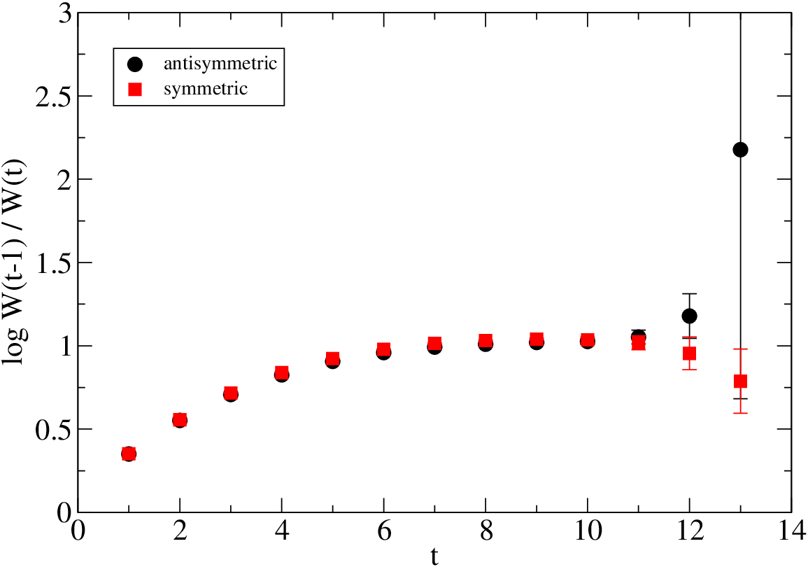
Finally, to check that the Lattice configurations are producing good results, we show the effective mass plot of a static potential in Fig. 10.
To conclude, we show that there are two, and only two, symmetric and antisymmetric, three-gluon static potential. We derive the two respective Wilson loops and study them analytically. We perform numerical tests, verifying that our Wilson loop is correct. Notice that the three-gluon Wilson loops include products of up to three fundamental Wilson loops, technically difficult to compute. We thus leave the systematic numerical exploration of the three-gluon Wilson loops for future works. Nevertheless, our numerical simulations already indicate that the symmetric potential is slightly larger than the antisymmetric one, and that both are compatible with the triangle-like model for the three-gluon static potential.
Acknowledgements.
Part of the present work was funded by the FCT grants PDCT/FP/63923/2005 and POCI/FP/81933/2007. We thank Orlando Oliveira for sharing with us his set of 141 configurations in a SU(3)QCD Lattice in part based on the MILC collaboration’s public Lattice gauge theory code [44, 45], and for scientific discussions.References
- [1] F. J. Llanes-Estrada, S. R. Cotanch, P. J. de A. Bicudo, J. E. F. Ribeiro and A. P. Szczepaniak, Nucl. Phys. A 710, 45 (2002) [arXiv:hep-ph/0008212].
- [2] H. B. Meyer and M. J. Teper, Phys. Lett. B 605, 344 (2005) [arXiv:hep-ph/0409183].
- [3] F. J. Llanes-Estrada, P. Bicudo and S. R. Cotanch, Phys. Rev. Lett. 96, 081601 (2006) [arXiv:hep-ph/0507205].
- [4] W. S. Hou and A. Soni, Phys. Rev. D 29, 101 (1984).
- [5] V. Mathieu, C. Semay and B. Silvestre-Brac, Phys. Rev. D 74, 054002 (2006) [arXiv:hep-ph/0605205].
- [6] F. Buisseret and C. Semay, Phys. Rev. D 76, 017501 (2007) [arXiv:0704.1753 [hep-ph]].
- [7] V. Mathieu, C. Semay and B. Silvestre-Brac, Phys. Rev. D 77, 094009 (2008) [arXiv:0803.0815 [hep-ph]].
- [8] N. Boulanger, F. Buisseret, V. Mathieu and C. Semay, arXiv:0806.3174 [hep-ph].
- [9] D. B. Leinweber, J. I. Skullerud, A. G. Williams and C. Parrinello [UKQCD Collaboration], Phys. Rev. D 60, 094507 (1999) [Erratum-ibid. D 61, 079901 (2000)] [arXiv:hep-lat/9811027].
- [10] P. J. Silva and O. Oliveira, Nucl. Phys. B 690, 177 (2004) [arXiv:hep-lat/0403026].
- [11] C. S. Fischer, R. Alkofer and H. Reinhardt, Phys. Rev. D 65, 094008 (2002) [arXiv:hep-ph/0202195].
- [12] H. B. Nielsen and P. Olesen, Nucl. Phys. B 61 (1973) 45.
- [13] C. Michael, Nucl. Phys. B 259, 58 (1985).
- [14] L. A. Griffiths, C. Michael and P. E. L. Rakow, Phys. Lett. B 129, 351 (1983).
- [15] A. Szczepaniak, E. S. Swanson, C. R. Ji and S. R. Cotanch, Phys. Rev. Lett. 76, 2011 (1996) [arXiv:hep-ph/9511422].
- [16] E. Abreu and P. Bicudo, J. Phys. G 34, 195207 (2007) [arXiv:hep-ph/0508281].
- [17] C. J. Morningstar and M. Peardon, Phys. Rev. D 60, 034509 (1999).
- [18] UKQCD Collaboration, G. S. Bali et al., Phys. Lett. B309, 378 (1993).
- [19] H. Chen, J. Sexton, A. Vaccarino, and D. Weingarten, Nucl. Phys. B34, 357 (1994).
- [20] M. Teper, hep-th/9812187 (1998).
- [21] N. A. Campbell, I. H. Jorysz and C. Michael, Phys. Lett. B 167, 91 (1986).
- [22] G. S. Bali, Phys. Rev. D 62, 114503 (2000) [arXiv:hep-lat/0006022].
- [23] F. Okiharu, H. Suganuma and T. T. Takahashi, Phys. Rev. D 72, 014505 (2005) [arXiv:hep-lat/0412012].
- [24] F. Okiharu, H. Suganuma and T. T. Takahashi, Phys. Rev. Lett. 94, 192001 (2005) [arXiv:hep-lat/0407001].
- [25] P. Bicudo, M. Cardoso and O. Oliveira, Phys. Rev. D 77, 091504 (2008) [arXiv:0704.2156 [hep-lat]].
- [26] M. Cardoso, P. Bicudo and O. Oliveira, PoS Lattice2007, 293 (2007) [arXiv:0710.1762 [hep-lat]].
- [27] O. Jahn and P. de Forcrand, Nucl. Phys. Proc. Suppl. 129, 700 (2004) [arXiv:hep-lat/0309115].
- [28] Ph. de Forcrand and O. Jahn, Nucl. Phys. A 755, 475 (2005) [arXiv:hep-ph/0502039].
- [29] T. T. Takahashi and H. Suganuma, Phys. Rev. Lett. 90, 182001 (2003) [arXiv:hep-lat/0210024].
- [30] H. Suganuma, T. T. Takahashi and H. Ichie, arXiv:hep-lat/0312031.
- [31] H. Suganuma, H. Ichie and T. T. Takahashi, arXiv:hep-lat/0407011.
- [32] T. T. Takahashi and H. Suganuma, Phys. Rev. D 70, 074506 (2004) [arXiv:hep-lat/0409105].
- [33] A. Yamamoto and H. Suganuma, Phys. Rev. D 77, 014036 (2008) [arXiv:0709.0171 [hep-ph]].
- [34] H. Suganuma, A. Yamamoto, N. Sakumichi, T. T. Takahashi, H. Iida and F. Okiharu, arXiv:0802.3500 [hep-ph].
- [35] A. Yamamoto, H. Suganuma and H. Iida, arXiv:0805.4735 [hep-ph].
- [36] B. Silvestre-Brac, C. Semay, I. M. Narodetskii and A. I. Veselov, Eur. Phys. J. C 32, 385 (2003) [arXiv:hep-ph/0309247].
- [37] P.G. de Gennes, Superconductivity of Metals and Alloys (Addison-Wesley, Reading, MA, 1989).
- [38] G. S. Bali, Schlichter and K. Schiling, Phys. Rev. D 51, 5165 ( 1995 )
- [39] G. Parisi, R. Petronzio, and F. Rapuano, Phys. Lett.. B 128, 418 ( 1983 )
- [40] APE Collaboration ( M. Albanese et al ), Phys. Lett. B 192, 163 ( 1987 )
- [41] F. Okiharu and R. M. Woloshyn, Eur, Phys. J. C35, 537 (2004)
- [42] T. T. Takahashi, H. Suganuma, Y. Nemoto and H. Matsufuru, Phys. Rev. D 65, 114509 (2002)
- [43] G. S. Bali, H. Neff, T. D�ssel, T. Lippert and K. Schilling, Phys. Rev. D 71, 114513 (2005)
- [44] This work was in part based on the MILC collaboration’s public Lattice gauge theory code. See http://physics.indiana.edu/sg/milc.html.
- [45] T. Blum, C. DeTar, S. Gottlieb, K. Rummukainen, Urs M. Heller, J. E. Hetrick, D. Toussaint, R. L. Sugar, M. Wingate, Phys. Rev. D55, R1133 (1997).