Experimental observables near a nematic quantum critical point
in the pnictide and cuprate superconductors

Rapid and important progress has been made in studies of Iron-oxypnictides superconductors. Various samples with similar FeAs plane and rare earths have been synthesized and several different compounds have shown superconductivity over 50K [1, 2, 3, 4, 5, 17], when the parent compound is doped by either fluorine or oxygen deficiency. Although many experimental facts, including the pairing symmetry, are still under debate, all these different samples share common features: a tetragonal-monoclinic (orthorhombic) lattice distortion and $(\pi,0)$ spin density wave (SDW) which commonly exist in the undoped samples, and “compete” with superconductivity at finite doping. The SDW and lattice distortion were first observed in $\mathrm{LaFeAs(O_{1-x}F_{x})}$ by elastic neutron scattering and X-ray spectroscopy [6]. Later on this phenomenon was confirmed in many other samples with La replaced by Ce [7], Sm [17, 18] and Nd [19, 20], and also in oxygen free materials $\mathrm{BaFe_{2}As_{2}}$ [8, 9], $\mathrm{SrFe_{2}As_{2}}$ [12, 13], and $\mathrm{CaFe_{2}As_{2}}$ [15, 16]. In all the samples, at the lattice distortion temperature $T_{c1}$, the resistivity shows a $\lambda$ shaped anomaly; therefore the $\lambda$ anomaly of resistivity can be taken as a measure of the lattice distortion in experiments.

Both lattice distortion and SDW are suppressed under doping, but, in general, the lattice distortion occurs at higher temperature than the SDW. In $\mathrm{SmFeAsO_{1-x}F_{x}}$, the lattice distortion and superconductivity coexist in a finite range of doping; the lattice distortion temperature seems to vanish within the superconducting phase [17, 18], while the coexistence between SDW and superconductor was never observed. In Ref. [21, 22], the lattice distortion is attributed to anisotropic antiferromagnetic correlation between electrons along $x$ and $y$ directions, without developing long range SDW. Since this order deforms the electron Fermi surface, equivalently, it can also be interpreted as electronic nematic order. This nematic order has Ising symmetry, therefore the transition temperature is controlled by the intralayer spin interaction, while the long range SDW is controlled by the interlayer spin interaction which is much weaker. Therefore the nematic transition (lattice distortion) occurs at a higher temperature than the SDW in general, and unless very close to the critical point, the nematic transition at finite temperature should belong to the 2d Ising universality class. The distance between the lattice distortion temperature and the SDW temperature depends on the anisotropy between $ab$ plane and $c$ axis, which can be checked by comparing the anisotropy of different samples.

The intimate relation between the structure distortion and SDW phase proposed by Ref. [21, 22] has gained support from recent experiments. It is suggested by detailed X-ray, neutron and Mössbauer spectroscopy studies that both the lattice distortion transition and the SDW transition of $\mathrm{LaFeAs(O_{1-x}F_{x})}$ are second order [23], where the two transitions occur separately. However, in $\mathrm{AFe_{2}As_{2}}$ with $\mathrm{A=Sr,\ Eu,\ Ba,\ Ca}$, the structure distortion and SDW occur at the same temperature, and the structure distortion becomes a first order transition [10, 12, 13, 14, 16] (or a very steep second order transition [24]). These results suggest that the SDW and structure distortion are indeed strongly interacting with each other, and the structure distortion is probably induced by magnetism.

We also note that the importance of nematic ordering has also been discussed recently in the context of the cuprate superconductors [25, 26]. Our results below are presented in the context of the pnictides, but all of the scaling properties of the experimental observables apply equally to the cuprates.

We focus on the zero temperature nematic phase transition at finite doping, motivated by the experimental suggestion of the existence of structure distortion critical point within the superconducting phase of sample $\mathrm{SmFeAsO_{1-x}F_{x}}$ [17, 18]. By contrast, the SDW phase shows no overlap with the superconducting phase in all the samples studied so far, therefore we will generally ignore it except for noting that the transition from the SDW to the nematic order is likely an $z=1$ O(3) transition, based on the fact that the SDW order wave vector is independent of doping [7], so the low energy particle-hole excitations at the SDW wave vector vanishes rapidly with small doping and hence make no contribution to the damping of the SDW order parameter [21]. The universality class of the nematic transition strongly depends on the pairing symmetry of the superconducting phase. If it is an $s-$wave superconductor without nodes, the transition of nematic order will be an ordinary 3D Ising transition; while if the superconductor is $d-$wave, the gapless nodal particles may change the universality class of the nematic transition. The recent STM [27] and Andreev reflection measurement [28] suggest that $\mathrm{SmFeAsO_{1-x}F_{x}}$ has nodes in the cooper pair, and the spin susceptibility measured by Knight shift will tell us whether it is a $p-$wave or $d-$wave pairing. In our current work we assume a $d-$wave pairing. The universal behavior of the nematic transition in a $d-$wave superconductor was first studied in Ref. [25]. Recently the same theory was studied carefully, and it was shown that in the infrared limit there is a special fixed point with logarithmically diverging velocity anisotropy of the nodal particles [26]. In the current work we will calculate experimentally relevant quantities close to this nematic quantum critical point. The global phase diagram is shown in Fig. 1.

The low energy Lagrangian describing the nematic order and nodal particle reads [25]

The Nambu fermion $\Psi$ is defined in the standard convention: $\Psi_{1a}=(f_{1a},\ \epsilon_{ab}f^{\dagger}_{3b})$ and $\Psi_{2a}=(f_{2a},\ \epsilon_{ab}f^{\dagger}_{4b})$. $a$ and $b$ are spin indices, $f_{1}$, $f_{2}$, $f_{3}$ and $f_{4}$ are slow fermion modes at nodal points $(Q,Q)$, $(-Q,Q)$, $(-Q,-Q)$ and $(Q,-Q)$ respectively. If the system develops long range order of $\phi$, the four nodal points of the $d-$wave superconductor will be shifted and break the $C_{4v}$ symmetry down to $C_{2v}$ due to the coupling $L_{\Psi\phi}$ [25]. The lagrangian (9) is not Lorentz invariant because in the real system $v_{\Delta}/v_{f}$ is in general not unity. Also, the coupling $L_{\Psi\phi}$ breaks the Lorentz invariance, since $\Psi^{\dagger}\tau^{x}\Psi$ is only one component of the space-time current of the Dirac fermion. Therefore a realistic scaling procedure is to allow $v_{\Delta}$ and $v_{f}$ flow independently under renormalization group (RG).

The nematic transition fixed point in Ref. [26] was obtained by expansion of $v_{\Delta}/(v_{f}N_{f})$, assuming a small initial value $v_{\Delta 0}/v_{f0}$, and in the current situation $N_{f}=2$. The RG flow of velocities is obtained by calculating the one-loop self-energy in Fig. 2$a$, with dressed $\phi$ propagator at order $1/N_{f}$ in Fig . 2$b$. The renormalization condition is chosen to be keeping the coupling constant $\lambda_{0}$ in $L_{\Psi\phi}$ invariant under RG flow. After the one-loop correction, the flow of the self-energy and velocities reads

$\Lambda$ is the momentum cut-off. $C_{1}$, $C_{2}$ and $C_{3}$ are functions of $v_{\Delta}/v_{f}$ and $N_{f}$, their detailed forms are given in the appendix. Using these RG equations, we are ready to calculate the scaling of the local density of states (LDOS) accessible by scanning tunneling microscope (STM):

$G_{1}$ and $G_{2}$ are retarded single particle propagator for $\Psi_{1}$ and $\Psi_{2}$. The RG equations in Eq. 16 are calculated by rescaling momentum cut-off. Since $v_{\Delta}/v_{f}$ is much smaller than 1 and flows to zero under RG, for frequency $\omega$, the corresponding momentum scale is $\tilde{p}=\omega/v_{f}$. Therefore $d\ln\omega/d\ln\tilde{p}=1+d\ln v_{f}/d\ln\tilde{p}$. Now the scaling equation for $\rho(\omega)$ reads:

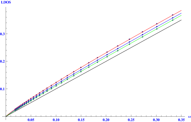
The ultraviolet cut-off of the theory is taken to be the transition temperature $T_{c}$ at the critical doping of nematic transition. Although $v_{\Delta}$ will be renormalized to be zero in the infrared limit, the expansion of $C_{2}$ and $C_{3}$ with small $v_{\Delta}/v_{f}$ given in Ref. [26] shows that $v_{\Delta}$ approaches zero slowly with energy scale, therefore for the experimentally relevant energy scale, one cannot naively take the fixed point value of $v_{\Delta}$. Instead, we have to integrate Eq. 30 numerically from the ultraviolet cut-off, and the result at certain frequency $\omega$ depends on the initial value of $v_{\Delta 0}/v_{F0}$. The results of $\rho(\omega)$ with initial value $v_{\Delta 0}/v_{F0}=1/5,1/10,1/20$ are plotted in Fig. 3, for frequency between $e^{-4}<\omega/T_{c}<e^{-1}$. unlike ordinary $d-$wave superconductor with LDOS $\rho(\omega)\sim\omega$, in all three plots the LDOS scales with frequency as

This simple power law relation fits well for the frequency range $e^{-4}<\omega/T_{c}<e^{-1}$, and it can be checked by STM technique on samples in the quantum critical regime.

The fluctuation of nematic order parameter certainly affects the thermal dynamical quantities. The free energy $\mathcal{F}=T\ln\mathcal{Z}/V$ has scaling dimension $d+z$, the singular part of the free energy can be written as

Now temperature is taken to be the infrared cut-off: $\xi_{\tau}\sim 1/T$, and the spatial correlation length can be estimated to be $\xi_{x}\sim v_{x}\xi_{\tau}$, $\xi_{y}\sim v_{y}\xi_{\tau}$. The anisotropic velocity of $\Psi_{i}$ leads to the following contribution to the free energy:

The $\phi$ contribution to the free energy and specific heat can be estimated in the same manner, although there is no velocity anisotropy for the $\phi$ field. The velocity of $\phi$ in the large $N_{f}$ limit can be evaluated by calculating the one loop correction to the self-energy of $\phi$. In the case of small $v_{\Delta}/v_{f}$, the velocity of $\phi$ can be taken to be $v_{f}$ isotropically:

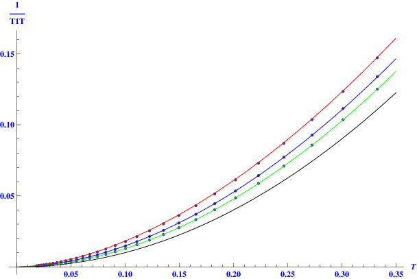
The solutions of Eq. 38 with different $v_{\Delta 0}/v_{F0}$ are plotted in Fig. 4. The equations are solved for the experimentally relevant temperature range $e^{-4}<T/T_{c}<e^{-1}$. In general, the nodal fermions contribute more to the specific heat compared with $\phi$ field, because $v_{\Delta}$ scales stronger with temperature compared with $v_{f}$. For $e^{-4}<T/T_{c}<e^{-1}$, the scaling of specific heat is

which distinguishes the current situation from the ordinary $d-$wave superconductor with nodes.

Another way to probe the density of states is the NMR relaxation rate $1/T_{1}$, which is related to the following Green function:

in the limit of $\omega\rightarrow 0$. The scaling of $1/(T_{1}T)$ with temperature is the same as the scaling of $F(\omega)$ with $\omega$, as $T$ and $\omega$ can both serve as infrared cut-off of the theory. The momentum integrated susceptibility should involve spin density at various “slow” momenta. At the low energy theory of the nodal particles, following fermion bilinears are low energy spin density modes that have universal scalings:

$\sigma^{a}$ are three spin Pauli matrices. To evaluate $F(\omega)$ we need to calculate the correlation of all the fermion bilinears above. The susceptibility $\chi$ gains fermion self-energy correction as in Fig. 2$a$ as well as vertex corrections Fig 2$c$ and Fig. 2$d$ for vertices $\Psi^{\dagger}_{i}T_{A}\Psi_{j}$ and $\Psi^{t}_{i}T_{A}\Psi_{j}$ respectively. For a general fermion bilinear with flavor matrix $T_{A}$, the vertex correction RG equation is conventionally written as

$C_{A}$ is a function of $v_{\Delta}/v_{f}$. The details of calculations are given in the appendix, the results are

$C_{0}$ is the vertex correction for fermion bilinear $\Psi^{\dagger}_{i}\Psi_{i}$ and $\Psi_{i}^{\dagger}\sigma^{a}\Psi_{i}$, because spin is a good quantum number spin Pauli matrices do not change the vertex correction. $C_{12A}$ and $C_{12B}$ are vertex corrections to $\Psi^{\dagger}_{1}\sigma^{a}\Psi_{2}$ and $\Psi^{t}_{1}\tau^{y}\sigma^{y}\sigma^{a}\Psi_{2}$, $C_{11}$ and $C_{22}$ are vertex corrections to $\Psi^{t}_{1}\tau^{y}\sigma^{y}\sigma^{a}\Psi_{1}$ and $\Psi^{t}_{2}\tau^{y}\sigma^{y}\sigma^{a}\Psi_{2}$ respectively.

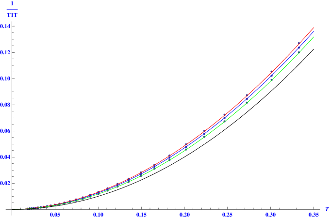
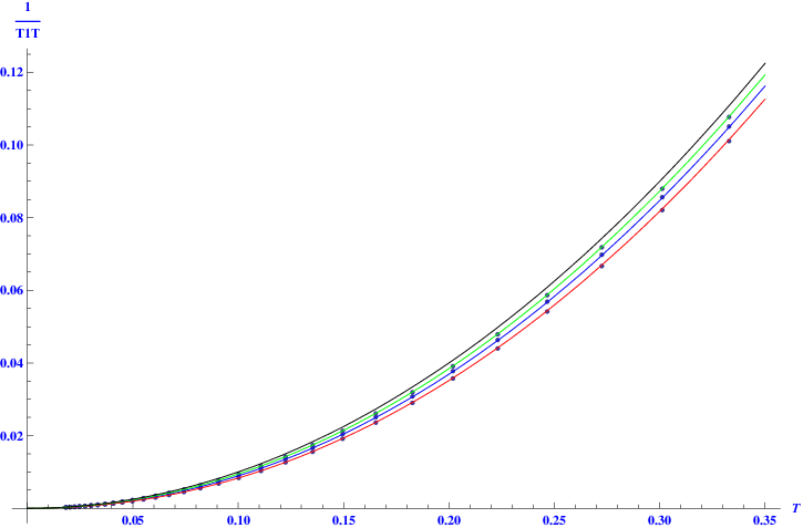
After taking into account of both self-energy and vertex corrections, the scaling equation of the relaxation rate reads:

Equation (72) leads to the following scaling equation for $1/(T_{1}T)$ with temperature:

The contribution from different fermion bilinear components listed in Eq. 60 should be solved individually, and the solutions of each component are plotted in Fig. 5, 6 and 7. One can see that at small frequency the spin density at $(0,0)$ makes the most substantial contribution, which makes the scaling of $1/(T_{1}T)$ differ from the ordinary $d-$wave superconductor:

The superconductivity can be fully suppressed by strong enough magnetic field. Since the nematic quantum critical point is most likely in the underdoped regime with low $T_{c}$, it is possible to apply strong enough inplane magnetic field $H>H_{c2}$ in experiments. With superconductivity fully suppressed by inplane magnetic field, the universality class of the nematic transition becomes the $z=3$ theory described in Ref. [21]. The $z=3$ quantum critical point leads to a large number of low energy excitations, which will contribute to thermal dynamics and transport. The standard mean field theory leads to following results at low temperature [21]:

These results will finally crossover to $d=3$ scalings close enough to the critical point:

Similar $z=3$ nematic quantum critical point was discussed in Ref. [29].

In a summary, in this work we computed the scaling of physical quantities close to a nematic quantum critical point in a $d-$wave superconducting phase of the newly discovered material $\mathrm{SmFeAsO_{1-x}F_{x}}$, motivated by recent experiments on the polycrystal sample. For the experimentally relevant energy range, the scaling of LDOS, specific heat, NMR relaxation rate all deviates from an ordinary $d-$wave superconductor. These results also apply, essentially unchanged, to the cuprate superconductors [25, 26]. This research is supported by the NSF under grant DMR-0537077.

References

- [1] Linjun Li, Yuke Li, Zhi Ren, Xiao Lin, Yongkang Luo, Zengwei Zhu, Mi He, Xiangfan Xu, Guanghan Cao, Zhu’an Xu, arXiv:0806.1675 (2008).
- [2] Zhi-An Ren, Jie Yang, Wei Lu, Wei Yi, Guang-Can Che, Xiao-Li Dong, Li-Ling Sun, Zhong-Xian Zhao, arXiv:0803.4283 (2008).
- [3] Zhi-An Ren, Guang-Can Che, Xiao-Li Dong, Jie Yang, Wei Lu, Wei Yi, Xiao-Li Shen, Zheng-Cai Li, Li-Ling Sun, Fang Zhou, Zhong-Xian Zhao, EuroPhys. Lett. 83, 17002 (2008).
- [4] X. H. Chen, T. Wu, G. Wu, R. H. Liu, H. Chen, D. F. Fang, Nature 453, 761 (2008).
- [5] Linjun Li, Yuke Li, Zhi Ren, Xiao Lin, Yongkang Luo, Zengwei Zhu, Mi He, Xiangfan Xu, Guanghan Cao, Zhu’an Xu, arXiv:0806.1675 (2008).
- [6] Clarina de la Cruz, Q. Huang, J. W. Lynn, Jiying Li, W. Ratcliff II, J. L. Zarestky, H. A. Mook, G. F. Chen, J. L. Luo, N. L. Wang, Pengcheng Dai, Nature 453, 899 (2008).
- [7] Jun Zhao, Q. Huang, Clarina de la Cruz, Shiliang Li, J. W. Lynn, Y. Chen, M. A. Green, G. F. Chen, G. Li, Z. Li, J. L. Luo, N. L. Wang, Pengcheng Dai, arXiv:0806.2585 (2008).
- [8] Marianne Rotter, Marcus Tegel, Dirk Johrendt, arXiv:0805.4630 (2008).
- [9] N. Ni, S. L. Bud’ko, A. Kreyssig, S. Nandi, G. E. Rustan, A. I. Goldman, S. Gupta, J. D. Corbett, A. Kracher, P. C. Canfield, arXiv:0806.1874 (2008).
- [10] Q. Huang, Y. Qiu, Wei Bao, J.W. Lynn, M.A. Green, Y. Chen, T. Wu, G. Wu, X.H. Chen, arXiv:0806.2776 (2008).
- [11] Marianne Rotter, Marcus Tegel, Inga Schellenberg, Wilfried Hermes, Rainer P02ttgen, Dirk Johrendt, arXiv:0805.4021 (2008).
- [12] C. Krellner, N. Caroca-Canales, A. Jesche, H. Rosner, A. Ormeci, C. Geibel, arXiv:0806.1043 (2008).
- [13] J.-Q. Yan, A. Kreyssig, S. Nandi, N. Ni, S. L. Bud’ko, A. Kracher, R. J. McQueeney, R. W. McCallum, T. A. Lograsso, A. I. Goldman, P. C. Canfield, arXiv:0806.2711 (2008).
- [14] Jun Zhao, W. Ratcliff II, J. W. Lynn, G. F. Chen, J. L. Luo, N. L. Wang, Jiangping Hu, Pengcheng Dai, arXiv:0807.1077 (2008).
- [15] Milton S. Torikachvili, Sergey L. Bud’ko, Ni Ni, and Paul C. Canfield, arXiv:0807.0616 (2008).
- [16] A.I. Goldman, D.N. Argyriou, B. Ouladdiaf, T. Chatterji, A. Kreyssig, S. Nandi, N. Ni, S. L. Bud’ko, P.C. Canfield, R. J. McQueeney, arXiv:0807.1525 (2008).
- [17] R. H. Liu, G. Wu, T. Wu, D. F. Fang, H. Chen, S. Y. Li, K. Liu, Y. L. Xie, X. F. Wang, R. L. Yang, L. Ding, C. He, D. L. Feng, X. H. Chen, arXiv:0804.2105 (2008).
- [18] Serena Margadonna, Yasuhiro Takabayashi, Martin T. McDonald, Michela Brunelli, G. Wu, R. H. Liu, X. H. Chen, Kosmas Prassides, arXiv:0806.3962 (2008).
- [19] Y. Qiu, Wei Bao, Q. Huang, J.W. Lynn, T. Yildirim, J. Simmons, Y.C. Gasparovic, J. Li, M. Green, T. Wu, G. Wu, X.H. Chen, arXiv:0806.2195 (2008).
- [20] Ying Chen, J. W. Lynn, J. Li, G. Li, G. F. Chen, J. L. Luo, N. L. Wang, Pengcheng Dai, C. dela Cruz, H. A. Mook, arXiv:0807.0662 (2008).
- [21] Cenke Xu, Markus Mueller, Subir Sachdev, Phys. Rev. B 78, 020501(R) (2008).
- [22] Chen Fang, Hong Yao, Wei-Feng Tsai, JiangPing Hu, Steven A. Kivelson, Phys. Rev. B 77 224509 (2008).
- [23] M. A. McGuire, A. D. Christianson, A. S. Sefat, B. C. Sales, M. D. Lumsden, R. Jin, E. A. Payzant, D. Mandrus, Y. Luan, V. Keppens, V. Varadarajan, J. W. Brill, R. P. Hermann, M. T. Sougrati, F. Grandjean, G. J. Long, arXiv:0806.3878 (2008).
- [24] Marcus Tegel, Marianne Rotter, Veronika Weiss, Falko M. Schappacher, Rainer Poettgen, Dirk Johrendt, arXiv:0806.4782 (2008).
- [25] Eun-Ah Kim, Michael J. Lawler, Paul Oreto, Subir Sachdev, Eduardo Fradkin, Steven A. Kivelson, Phys. Rev. B 77, 184514 (2008).
- [26] Yejin Huh, Subir Sachdev, arXiv:0806.0002 (2008).
- [27] Oded Millo, Itay Asulin, Ofer Yuli, Israel Felner, Zhi-An Ren, Xiao-Li Shen, Guang-Can Che, Zhong-Xian Zhao, arXiv:0807.0359 (2008).
- [28] Yonglei Wang, Lei Shan, Lei Fang, Peng Cheng, Cong Ren, Hai-Hu Wen, arXiv:0806.1986 (2008).
- [29] Vadim Oganesyan, Steven Kivelson, Eduardo Fradkin, Phys. Rev. B 64, 195109 (2001).