![[Uncaptioned image]](0807.1501v1/frontesp.png)
![[Uncaptioned image]](0807.1501v1/title.png)
Part I On the QCD coupling at low energy scales
Chapter 1 The QCD coupling in Perturbation Theory
The Renormalization Group method is an inherent part of the theoretical
description of strong interaction processes. As known, the values of the
QCD coupling extracted from high-energy data are in good agreement with
the theoretical running coupling as derived by the RG
equations and properly normalized at the boson mass, thus providing
a powerful test of asymptotic freedom 11
1
For a summary of the high energy
mesurements of see [1, 2]..
On the other hand, in the low-energy domain, the running coupling
develops, at any loop level, unphysical (so-called Landau) singularities that
contradict
the general principles of the local Quantum Field Theory and severely
complicate the theoretical analysis of hadron dynamics.
A reasonable prescription to get rid of the Landau singularities in the
QCD coupling is given by the Analytic Perturbation
Theory (APT) approach. In this framework, the analycity properties are
recovered by imposing
to satisfy a dispersion relation with only the unitary
cut on the time-like
axis, while preserving the asymptotic freedom constraint.
This prescription has been exploited in the framework of a second order
Bethe-Salpeter-like (BS) formalism adjusted for QCD in recent
works [24], for the calculation of the meson spectrum in the light and
heavy quark sectors. It has been there enphasized the relevance of the
infrared evolution of the APT coupling in the few hundreds MeV
region for a reasonable reproduction of ground state mesons involving light
and strange quarks,
at variance with a naive truncation prescription.
This feature strongly supports the APT approach within the BS framework.
On the other hand, in the present work [3, 4],
the calculations of the meson
spectrum
within the BS formalism have been exploited in order to obtain an experimental
determination
of the strong coupling below 1 GeV, by comparison with
the data.
The results turn out to be in satisfying agreeement with
the APT coupling and its evolution in the 200-500 MeV region. Furthermore, below this
scale, some hints on the deep IR behavior are further provided, albeit affected
by large theoretical errors.
In Sec. 1 the Renormalization Group method in QCD is briefly reviewed, and the
state-of-the-art on the infrared behavior of the QCD-invariant coupling sketched,
whereas in Sec. 2 the basis of the Analytic Perturbation Theory approach are
outlined.
Sec. 3 is devoted to the determination of the experimental values of the QCD coupling
from the meson spectrum, the analysis method and the discussion of the results.
Finally, some technical material is exposed in the Appendices. A short description
of the derivation of the second order BS formalism is given in App. A, whereas
numerical tables in App. B display all the results in detail.
1.1 The Renormalization Group method in QCD
In the framework of Quantum Field Theory,
an arbitrary change in the renormalization prescription basically
results in a reparametrization of the theory by a suitable
redefinition of couplings and masses, so as to leave physical
quantities unaffected. The behavior of relevant
Green functions under a change in the extra mass scale introduced
by renormalization is specified by a set of
continuous transformations, properly expressed by the differential
equations of the renormalization group (RG) 22
2
For an
overview on history and applications see for
instance [5] and references therein.. This leads to the notion
of effective couplings and masses.
Choosing a renormalization scheme (RS) which performs all
subtractions off shell, mass parameters can be treated on the same
foot as couplings.
In the “minimal subtraction scheme” (MS)
the renormalization factors exhibit no mass-dependence and are of the
general form
| (1.1) |
where is the strong coupling and is the
deviation from
the physical space-time dimension, .
The so-called “modified minimal substraction scheme” ()
amounts to subtracting the whole -term together with
the poles, and it has become a common standard in QCD.
In MS-like schemes the arbitrary mass scale arises to keep the
coupling dimensionless in dimensions, and the
renormalized objects turn out to be scale dependent.
In transition from one parametrization
to a different one
Green functions are connected by finite renormalization transformations,
and, in order to have a unique theory
under an infinitesimal shift of the scale, they
must satisfy the (inhomogeneous) RG equation
| (1.2) |
where are relevant momenta and the shorthand stands for (similarly for ). The RG operator is the total derivative over the scale parameter, namely
| (1.3) |
where the sum over quark flavors in the mass-term is understood, and the universal functions
| (1.4) |
have been defined. The RG coefficients and are computed in perturbation theory (PT) with the aid of the relative counterterms. Generally speaking, they are gauge-dependent finite functions of couplings and masses, once the physical limit is performed; actually, in any mass-independent RS (such as minimal subtraction prescriptions or trivially in massless theories), the RG coefficients are mass-independent and function of alone.
As far as the QCD coupling is concerned, the beta function in the first of Eqs. (1.4) has the usual PT power expansion
| (1.5) |
where are the l-loop coefficients. At 1-loop level (i.e. keeping only the first term in (1.5)) solution to the first of Eqs. (1.4) reads
| (1.6) |
namely, while the theory does not predict the actual size of ,
its scale evolution is completely known. Indeed,
is not an observable by itself, but plays the role of the effective
expansion parameter for physical quantities, and any determination of the
strong coupling is
then extracted from the measurements of observables for which PT
predictions exist. Conventionally the mass of the boson,
GeV,
is used as a reference scale to the world average
of all (high energy) determinations, which is currently
[2, 1].
Defining the overall scale parameter
| (1.7) |
Eq. (1.6) becomes
| (1.8) |
Since is a positive number for all presently known flavours, decreases to zero as (asymptotic freedom), this property being not spoiled by higher loop corrections.
Given the arbitrariness of the renormalization scale , the best choice is a matter of expediency. The commonly adopted prescription is to fix at the physical scale of the process at hand. This can be motivated by a glance to the homogeneous RG equation satisfied by any (dimensionless) observable , namely 33 3 Actually quark masses have been neglected, assuming that both the physical and the renormalization scales and are larger than any other relevant mass scale. If non negligible, quark masses give rise to an additional term in Eq. (1.9), similarly to Eqs. (1.2) and (1.3).
| (1.9) |
where is typically function of the ratio 44 4 Actually, according to the process, more than one scale can be involved, and this can be spacelike ( and ) or timelike ( and ). and of the renormalized coupling , and is given in PT by a power series in
| (1.10) |
Eq. (1.9) clearly states the scale invariance of
any physical observable, that is fulfilled only in infinite order.
In any truncated order, however, the cancellation of the scale
among the coupling and the coefficients is not complete, that is,
a residual scale and scheme dependence still persists, and the
degree of cancellation improves with the inclusion of higher orders.
The solution of Eq. (1.9) for the PT coefficients exhibits a
logarithmic dependence on (starting from the order ),
that can be controlled by setting . Then Eq. (1.10) takes
the form
| (1.11) |
and the energy dependence of translates into the energy dependence of the effective parameter . A change in the value of clearly amounts to a reorganization of the PT expansion.
The RG improved perturbative QCD yields a consistent picture of high energy
strong interaction processes 55
5
Some care is required
for timelike observables since the PT coefficients, in this case, are modified
by non negligible corrections, proportional to powers of , due
to the analytic continuation fron the space-like to the time-like domain (see
Sec. 1.6). from a few GeV
up to a few hundred GeV. On the other hand, the
existence of infrared singularities
in the RG-invariant coupling spoils the theoretical
analysis of low energy hadron dynamics.
Indeed, at 1-loop level , as given by Eq. (1.8), has
a pole-type
singularity at , and the effect of including higher order
contributions
does not overcome the problem and only amounts to modifying
the singularity structure.
On the contrary, physical observables are known to be analytic in the entire
complex plane aside from a cut on the real positive (time-like) axis, and
their exact expressions should be free of these singularities.
Many strategies have been suggested to get rid of unphysical singularities
within PT calculations, so as to handle the strong interaction processes at
low energies. Some of such methods, reviewed e.g. in Ref. [6],
originate in the general properties of the perturbative power series for the QCD
observables in the framework of the RG formalism, such as the arbitrariness of
the renormalization scheme and scale. One can
remind, for instance, the Brodsky-Lepage-Mackenzie criterion [7],
the “Optimal conformal mapping method” [8]
(see also Ref. [9]), and the so-called “Fastest Apparent Convergence”
technique [10]. The latter, e.g. amounts to setting the scale so
that all the higher (than LO) coefficients vanish. It is related to
the effective charges, [11]-[13],
i.e. alternative definitions of the QCD coupling, straightforwardly related
to a physical
observable, either of spacelike or time-like argument.
In this context it is also worth mentioning the “Optimized Perturbation Theory”
approach [14, 15], with the aim of improving the convergence of PT
expansions by a proper choice of the scale and of RS parameters (such as
and ), on the basis of a minimum sensitivity criterion.
However, all these definitions can be related to each other by referring back
to the conventional .
Most of these techniques yield theoretical predictions
on the low energy behavior of the RG-invariant coupling which are in qualitative
agreement, suggesting in all cases an IR finite limit.
Furthermore, recent results of lattice simulations testify to the absence of spurious
IR singularities in the QCD coupling [16, 17].
The ghost-pole issue gives rise to severe complications, in particular,
as far as the bound states problem is concerned, since the characteristic
scale involved (i.e., the momentum transfer in the quark-antiquark
interaction for mesons) is typically below 1 GeV, according to the
state and the mass of quarks involved.
Among the many potential inspired attempts to modify the expression of
in the low energy domain, there exist either trivial tricks
as the trucation prescription 66
6
This simply amounts to assuming
frozen at a maximum finite value in the IR region., as well as
more sophisticated models. For instance, one can remind the 1-loop definition
of the QCD coupling
in connection with the momentum
representation of the Cornell-like potential [18]
| (1.12) |
as , the usual 1-loop coupling (1.8) is recovered from the first of Eqs. (1.12), whereas as the latter diverges as , incorporating non-perturbative effects 77 7 This can be seen by comparing the second of (1.12) with the usual Cornell potential in the momentum space representation (1.13) and identifying the quantity with the string tension that controls the confining part of the potential.. Estimation of higher order corrections and further developments along this line can be found in [19]. On the other hand, a number of analyses seems rather consistent with an IR finite coupling and a suitable modification of the quark-antiquark potential to encode confinement (see e.g. [20, 21, 22, 27]).
A reliable algorithm to get rid of Landau singularities is provided by the Analytic Perturbation Theory (APT) approach [23], which represents a next step, after RG summation, in improving the perturbative results. The APT method, as discussed to some extent in Sec. 2, is based on the causality condition which imposes the analyticity constraint on the RG-invariant coupling on the whole cut complex plane . PT is then used to evaluate the spectral function, i.e. the discontinuity of across the cut. At 1-loop, e.g., it reads
| (1.14) |
where Eq. (1.6) has been used. Indeed, within the causal approach, Landau singularities are suppressed at their very roots, and the IR-safe QCD coupling possesses a universal finite limit as .
In what follows the basis of the derivation of the QCD coupling from the Renormalization Group equations are reviewed, both in the space-like and time-like domains.
1.2 QCD function
The RG equation for the effective coupling is actually solved in PT with the aid of the relation
| (1.15) |
where the limit is understood. Thus one needs to compute the renormalization factor for the coupling and this can be accomplished in several ways. One can start from the quark-gluon vertex together with renormalization factors of quark and gluon propagators and to obtain , but other choices, as ghost-ghost-gluon vertex or trilinear and quartic gluon interactions, equally work. In a minimal subtraction prescription the four-dimensional -function is entirely specified by the residuum of the simple pole in the -expansion of (1.1)
| (1.16) |
Then the MS-coefficients in Eq. (1.5) reads [29]
| (1.17) |
where is the Riemann zeta-function, .
The coefficients generally depend on the RS,
whereas the first two are universal within massless schemes.
Moreover, in the -scheme the -function is
gauge-independent in any order [30], and in an
arbitrary mass-dependent scheme this feature is preserved only
in the first order.
As already noted, the universal 1-loop coefficient [31]
has a positive sign provided there is a small enough number of quark
fields ; thus the theory is asymptotically free, that
is, the -function has a stable UV fixed point as its argument
decreases to zero. Indeed this coefficient is the sum of two
contributions, the relevant one with respect to asymptotic freedom
property being the first, which arises from pure gauge field
effects i.e. from the nonlinear Yang-Mills interaction terms. The
2-loop coefficient has been computed for the first time
in [32] and is positive up to .
Higher order approximations are scheme-sensitive, and it is common
practice to perform computation within minimal subtraction prescriptions,
in which the -function is unchanged. The first
calculation of 3-loop coefficient is due to [33],
where the ghost-ghost-gluon vertex in the Feynman gauge was used, and
it turns out to be negative for .
In a more recent work [34] the quark-gluon vertex
was used instead, providing an independent check in an arbitrary
covariant gauge of the previous result and its gauge-independence.
Finally, the original 4-loop calculation [29]
has been performed using the ghost-ghost-gluon vertex in a arbitrary
covariant gauge, and for a generic semi-simple compact Lie symmetry
group. The result turns out to be gauge-independent, and involves
higher order group invariants
such as quartic Casimir operators; specialized to the standard
SU(3) symmetry, the 4-loop coefficient is a positive number
for every positive (see also [35]).
Finally note that (except for ) all four coefficients
are positive up to .
1.3 RG-invariant coupling
The formal solution of the first of Eq. (1.4) is easily worked out
| (1.18) |
and yields the evolution of the effective coupling as a function of two dimensionless arguments and , where can be viewed as a fixed reference scale and as a sliding one. It is worth noting that by differentiating Eq. (1.18) with respect to one has
| (1.19) |
namely the homogeneous RG equation satisfied by the effective coupling
(or invariant charge).
The exact 1-loop solution (1.6) or (1.8) is
obtained by retaining only the first
term in (1.5). In Eq. (1.8), in particular,
the dimensional scale keeps track of the
initial parametrization , and it
is scale-invariant; its value is not predicted by the theory
but must be extracted from a measurement of at a
given reference scale.
Emergence of a scale parameter, sometimes referred to as dimensional
transmutation, breaks naive scale invariance of the massless theory,
and it is commonly believed to be associated with the typical hadron
size i.e. to the energy scale where confinement effects set in.
Roughly speaking, is the scale at which the (1-loop) coupling
diverges (Landau pole), and perturbation
theory becomes meaningless. Further, is scheme-dependent and receives
further corrections at each loop level (but for simplicity the
same notation is used throughout).
At the 2-loop level the integration of (1.18) leads to a transcendental equation, that is, starting from the 2-loop approximation to the -function in (1.5), one has
| (1.20) |
where and the constant term from the lower end points can be again reabsorbed into the -parametrization, with the commonly adopted prescription (see e.g.[36, 37])
| (1.21) |
which fixes a specific choice for . Thus one gets the 2-loop implicit solution
| (1.22) |
from which the 2-loop scaling parameter is immediately read. To achieve an explicit expression for the running coupling at this level one should resort to the many-valued Lambert function implicitly defined by the equation
| (1.23) |
The function has an infinite number of branches such that (for more details see [38]). The exact solution to Eq. (1.22) for reads 88 8 Note that if the principal branch is involved, but here and throughout the discussion is focused on . (see e.g. [39])
| (1.24) |
where , and is the “physical” branch of the Lambert function, since it defines a real values function for which fulfills the asymptotic freedom constraint. As the asymptotic relations
| (1.25) |
| (1.26) |
hold. Outside this region of the real axis
takes on complex values.
Though not easy for practical aims, Eq. (1.24) yields
the most accurate expression for investigating the IR behavior of
the running coupling, since it has not been derived by means of deep
perturbative approximations (aside from the truncation of the 2-loop
function).
Actually, a frequently used 2-loop approximate solution, known as the
iterative solution [23], is obtained
starting from Eq. (1.20) together with a single iteration
of the 1-loop formula (1.8), that is
| (1.27) |
where , and now defined in (1.20) by
| (1.28) |
This definition is related to the standard one (1.21) by the factor
| (1.29) |
However, the commonly used 2-loop solution is an asymptotic formula which strictly relies on the smallness of for fairly large , since it amounts to solving Eq. (1.20) (with the choice (1.21)) where the last term in the r.h.s. has been neglected. Again, after one iteration of the 1-loop formula, the result is then re-expanded in powers of , where and as before
| (1.30) |
Eq.(1.30) is known as the standard 2-loop running coupling and works only in the deep UV regime, i.e. for . In Fig. 1(a) the fractional differences of the two approximate formulas Eqs. (1.27) and (1.30) with respect to the exact 2-loop coupling Eq. (1.24) are displayed.
Under the same assumptions of Eq. (1.30) one can easily derive the 3 and 4-loop asymptotic formulas. Starting with the approximate implicit solution at the 4-loop level, namely
| (1.31) |
the 4-loop coupling in the standard form of an expansion in inverse powers of the logarithm for (see e.g. [40]) reads
| (1.32) |
The 4-loop solution (1.32) turns out to be nearly indistinguishable
from the 3-loop curve (see Fig. 1(b)).
In Eq. (1.32) the 1-loop solution (1.8) has been
emphasized, and being the leading UV term in (1.32), it
defines the asymptotic behavior of the RG-invariant coupling.
On the other hand, the 2 and 3-loop asymptotic expressions are
easily read from Eq. (1.32) by
keeping only the first two and three terms respectively.
Exact integration of the truncated 4 or 3-loop -function leads to a more involved structure than Eq. (1.31). Nevertheless, in [39] a useful solution has been still worked out at 3-loop level via the real branch of the Lambert function together with the Pade’ Approximant of the related -function. Moreover, in [41] a reliable approximation to the higher-loop coupling has been suggested, via a power expansion in the 2-loop exact coupling (1.24), of the form
| (1.33) |
with the loop order, and proper functions of the coefficients . Comparison [42] of these multi-loop approximants with the relative asymptotic formulas, Eq.(1.32) and the 3-loop analogue, reveals the better agreement of the former ones with the higher-loop exact coupling numerically estimated (i.e. starting from the exact implicit solution), even at rather low energy scales (see also [43]).
Finally, as far as the definition of the scaling constant
is concerned, few comments are in order. As already
pointed out, starting from the 2-loop level an arbitrary
constant has to be fixed for to be uniquely defined;
beside the commonly accepted convention (1.21)
(or (1.28)), other prescriptions
have been proposed [44] in order to optimize the
-expansion, while (1.21)
does remain the preferred one as no further terms of order
appear in the 2-loop asymptotic formula (1.30).
Thus, at higher-loop levels the scaling parameter is analogously
related to the initial parameterization, and the 4-loop (and 3-loop)
value reproducing the world average is
MeV [1].
Furthermore, with regard to the scheme-dependence of the coupling and
the scale parameter, restricting the discussion to mass-independent
RS (as MS-like schemes or trivially any prescription in the
massless theory), the renormalized couplings in two such different schemes can be related
perturbatively at any fixed scale
| (1.34) |
Then, it can be verified that the first two coefficients of the relative -functions do not change as the renormalization prescription is changed, while, for instance, the 3-loop ones are related by . As a result, the runing coupling at each loop-level (e.g. Eq. (1.32)) depends on the RS, through the coefficients with and the initial parameterization. The latter obviously amounts to suitably adjusting the , and the relation is given by [45]
| (1.35) |
which works through all orders (e.g. ).
1.4 Threshold matching
Quark mass effects reveal themselves in
explicit corrections within higher order perturbation theory
(see e.g. [46]), and in the energy
dependence of the effective (running) quark masses as a
result of the RG improvement [47].
A direct effect of the quark masses
on the evolution of the coupling is through
the dependence of the coefficients on the number
of active quarks, i.e. satisfying ,
where is the renormalization scale and the
quark mass (the definition can be also
formulated in terms of the pole mass that can be
related to the former [48]).
Then, in order to have a continuous coupling on the whole
domain, the two functions and
must be matched at each heavy quark
mass scale . As a result the scaling
parameter depends also on (see
e.g. [49, 40]).
The most straightforward way is to impose continuity of
by means of the matching condition
,
which works up to next-to-leading order. At 1-loop,
it yields
| (1.36) |
that can be extended up to 2-loop, and exhibits explicit dependence on . Since trivial matching does not generally hold in higher orders within scheme, a more accurate formula is required in this case; specifically to obtain the global evolution of the 4-loop coupling the proper matching condition reads [40]
| (1.37) |
with
| (1.38) |
if is exactly assumed. With this convention,
Eq. (1.37) yields the relationship between
and in the
scheme.
One can equally fix , that amounts to a
proper adjustment of the coefficients in (1.37); for
instance [1] starting with (1.32) and
MeV, the values
MeV and MeV are
obtained, with thresholds fixed at the pole masses GeV
and GeV.
Note finally that Eq. (1.37) spoils
continuity of ; therefore,
one can resort to a more sophisticated
technique [50], which relies upon mass-dependent
RS and yields a smooth transition across thresholds.
1.5 Landau singularities
As already noted, the 1-loop coupling (1.8) is affected by a
spacelike pole at with residue .
Adding multi-loop corrections does not overcome the
hurdle; rather, the singularity structure
is more involved due to the log-of-log dependence,
so that a branch cut adds on to the 1-loop single pole in the IR
domain of the spacelike axis.
Moreover, at a given loop level, Landau singularities sensibly
depend on the approximation used. For instance, the 2-loop
iterative formula (1.27) has a pole at
(, see Eqs. (1.28) and (1.29))
with residue , and a cut for due
to the double logarithm. On the other hand, in the 2-loop
asymptotic expression Eq. (1.30), the singularity
in becomes stronger, namely
| (1.39) |
and the cut now runs from 0 to 1. Analogously, the 3- and 4-loop asymptotic solutions, as given by Eq. (1.32), behave as
| (1.40) |
and are equally affected by an unphysical cut. However, the cumbersome singularities structure of the leading Landau singularity, and of the unphysical cut as well, are an artifact of the UV approximations introduced. Therefore to deal with the IR behavior of the invariant coupling it is necessary to face with the exact solution, e.g. Eq. (1.24) at 2-loop; clearly it is singular when that is at (), corresponding to the branch point of the Lambert function. In the neighborhood of this point, due to the asymptotic behavior (1.26) of , one has
| (1.41) |
i.e., an integrable singularity (the factor
in front of in the singular point can be reabsorbed
into a proper redefinition of the integration constant, through
Eq. (1.29)).
A more detailed investigation about the IR singularity structure
of higher-order approximations of the QCD coupling has been performed
in Ref. [43], on the basis
of Eq. (1.33), where, in particular, the location of Landau
singularities as a function of are studied.
1.6 Time-like coupling
The evolution of the QCD coupling has been derived above
in the space-like region.
However, in order to parametrize observables of time-like arguments,
one needs an effective coupling defined on the whole real axis.
While this poses no special problems in high energy processes,
at any finite energy the issue of which should be the most
suitable parameter in the s-channel must be carefully considered.
The standard practice is to
merely take over to the time-like domain the space-like coupling
at any loop level, regardless of the crossing between two
disconnected regions, thus exporting the IR singular
structure in the s-channel.
Nevertheless, from many early works based upon analysis of
-annihilation into hadrons (see [51] and
references therein),
it is known that this should not be the
case except far in the asymptotic regime. This is because of the
appearance of not negligible corrections (-terms) in the
higher order coefficients of the -expansions,
due to analytic continuation from space-like to time-like axis.
The problem is related to the IR non analyticity of the invariant
coupling, and it receives a satisfactory answer
in the framework of Analytic Perturbation Theory, in which
the space-like and time-like channels are treated in a unified description
(see Sec. 2).
Referring for definiteness to the -annihilation ratio into
hadrons
| (1.42) |
where , one can start with the hadronic contribution to the photon polarization tensor in (space-like) momentum space
| (1.43) |
being the quark electromagnetic current operator. As is known, exploiting the analytical properties of the two-point correlation function (1.43) in the cut complex plane , can be straightforwardly related to the discontinuity of across the cut
| (1.44) |
In order to compute on the space-like axis () one formally works with its first logarithmic derivative (thus avoiding subtraction constants), the Adler -function [52]
| (1.45) |
The RG improved PT expansion of the -function reads
| (1.46) |
where , are the quark charges, and the coeffcients in the scheme read [53]
| (1.47) |
Then, by integration, is readily obtained 99 9 In the massless case the cut spreads over the whole positive axis, while taking into account quark masses the cut starts at the two-pion threshold .. The result for is then usually recasted as a series in the effective parameter , naively obtained by specular reflection, that is by replacing the space-like argument with the time-like one . Starting from the series displays corrections proportional to powers, as a drawback of the analytic continuation of the hadronic tensor. Then the ordinary perturbative expansion for (e.g. [54]) reads
| (1.48) |
| (1.49) |
with and the same as in (1.46), and . The correction gives to the coefficient a strongly negative contribution for each (roughly for ). Higher order -terms were analyzed in [55] and show a remarkable growth; for instance, the fourth order correction is
| (1.50) |
with for .
A similar treatment also holds for other
s-channel observables [54], such as the normalized rate
for -decay into hadrons. The effects of analytic
continuation then make the perturbative expansions in the time-like region
different from Euclidean ones.
Since the -terms play a dominant role in higher order
coefficients, expansion (1.48) works only asymptotically at
large , that is when the smallness of scales
down these large contributions. Actually, as already noted in pioneer
works [56, 57],
the expression of , resulting from Eq. (1.44)
exhibits no natural
expansion parameter (since both real and imaginary parts of
enter into the expression of ), and its choice
is essentially a matter of expediency.
Alongside less meaningful attempts, one can remind e.g. the
analysis performed in Ref. [56] of the quantity
| (1.51) |
as expansion parameter for . Among the main features, Eq. (1.51) turns out to be IR finite, thus avoiding the hurdle of Landau singularities on the time-like domain, whereas asymptotically, i.e. for , it reads
| (1.52) |
resembling the UV behavior of the related space-like coupling (1.8). However, Eq. (1.51) cannot entirely sum up the -terms.
In order to deal with these corrections, a somewhat different approach, known as RKP (Radyushkin-Krasnikov-Pivovarov) procedure, has been suggested [44, 58] (see also [59]), which is based upon the analytical properties of the polarization tensor and of the related -function (1.45), that can be summarized by the dispersion relations, respectively
| (1.53) |
| (1.54) |
with given by (1.44), and lying in . The key point here is the inverse of Eq. (1.54), given by the contour integral
| (1.55) |
to be computed along a path in the analyticity region for the -function. Eq. (1.55) can be then generalized to an integral transformation, mapping a space-like argument function into a time-like one
| (1.56) |
This can be straightforwardly applied to the perturbative expansion (1.46), provided that the integration contour is always kept far enough from IR space-like singularities. This yields as an expansion into the images of and of its powers, through the map [44]
| (1.57) |
where the coefficients are the same as in Eq. (1.46). Eq. (1.57) is to be compared with the standard perturbative expansion (1.48); here the -terms are entirely summed up, with the drawback that, within this framework, there is no uniquely defined expansion parameter. However, it is useful to work out its behavior to for , namely
| (1.58) |
easily obtained by applying the integral transformation (1.55) to the 1-loop space-like coupling (1.8). The related time-like coupling (1.58) is free of unphysical singularities at low (as Eq. (1.51)), and for can be expanded into powers of
| (1.59) |
Then Eq. (1.59) can be recasted as a power series in the 1-loop space-like coupling
| (1.60) |
emphasizing that the space-like and time-like couplings differ at 3-loop level. The comparison between Eq. (1.60) and Eqs. (1.48) and (1.49) makes it clear the RKP resummation of the -terms into the time-like coupling (1.58). The main shortcoming of this recipe is that by applying to Eq. (1.58) the inverse transformation , i.e. relation (1.54), the original input (1.8) is not recovered. Obviously, this is because integral transformations (1.55) and its inverse are well-behaved as long as the integrand possesses the correct analytical properties in the cut complex plane; actually this is not the case for the space-like coupling (1.8) and its higher-loop approximations, and one is then forced to compute the integral along a path large enough to avoid the IR space-like singularities.
Chapter 2 The APT theoretical scheme
2.1 The “Euclidean” ghost-free coupling
The analytic approach constitutes the next step, after the RG-summation, in improving the perturbative results. Specifically, in addition to the property of renormalizability, this method retains a general feature of local QFT, the property of causality. The analytic approach has first been devised in the context of Quantum Electrodynamics [60], and then extended to the QCD case about ten years ago [23]. The basic merits of the analytic approach to QCD are the absence of unphysical singularities of the invariant charge and the enhanced stability of outcoming results with respect to both higher loop corrections and the choice of renormalization scheme [61]. Besides, this method enables one to process the spacelike and timelike data in a congruent way [62]. A fresh review of the analytic approach to QCD and its applications can be found in the paper [63].
Usually, in the framework of RG-improved perturbation theory a QCD observable of a single argument (spacelike momentum transfer squared) can be represented as a power series in the strong coupling (cf. Eq. (1.46)):
| (2.1) |
where are the relevant perturbative coefficients. However, in
the IR domain this expansion becomes inapplicable due to the spurious
singularities of the running coupling .
For example, the 1-loop expression (1.8)
possesses both the physical cut along the negative real semiaxis
and the unphysical pole at .
In the framework of the APT, the power series (2.1) for an
“Euclidean” observable is replaced [65] by the nonpower
expansion
| (2.2) |
over the set of functions
| (2.3) |
Here, the spectral function is defined as the discontinuity of the relevant power of the perturbative coupling across the physical cut, namely
| (2.4) |
The APT representation (2.2) for a QCD observable is free of spurious singularities. Besides, it displays a better stability, in comparison with the perturbative parameterization (2.1), with respect to both, the higher-loop corrections and the choice of the renormalization scheme (see Ref. [63] for details). The first-order function (2.3) plays the role of the effective Euclidean QCD coupling at a given loop level:
| (2.5) |
The argument now runs over the whole space-like axis, that is, is free of any space-like unphysical singularities by construction; moreover, due to the asymptotically free nature of the perturbative input the spectral integral (2.5) needs no subtractions.
In the 1-loop case this equation can be integrated explicitly [23]
| (2.6) |
The analytically generated non-perturbative contribution in Eq. (2.6) subtracts the pole in a minimal way, yielding a ghost-free behavior which avoids any adjustable parameter. Furthermore, for this non-perturbative term in Eq. (2.6) can be rewritten as
| (2.7) |
namely, as a series of power-suppressed corrections to the 1-loop
perturbative coupling (1.8). Since
the pure perturbative
contribution dominates in the deep UV region, the asymptotic
freedom constraint of the invariant coupling is preserved.
On the other hand, Eq. (2.6)
exhibits the infrared finite limit
(roughly 1.4,
if ).
This value turns out to be independent of the QCD scale , and
it is also universal with respect to higher-loop corrections,
warranting a remarkably stable IR behavior of (2.6).
Obviously the scaling parameter has now to be re-defined as
| (2.8) |
where the function is the formal inverse of (2.6), that is, it satisfies the equation
| (2.9) |
with and . In a similar way, the beta-function for the 1-loop coupling (2.6) reads [23]
| (2.10) |
with again given by Eq. (2.9). Despite the implicit form of (2.10), the symmetry property reveals the existence of a IR fixed point at , corresponding to the IR finite limit (see also [66]).
2.2 Two-loop and higher orders
Actually, as discussed in Sec. 1.3, the
RG equation for the invariant coupling has no simple
exact solution beyond the 1-loop level, and asymptotic expressions
are commonly used (Eq. (1.32)), with a
cumbersome IR nonanalytical structure. As a result, the
spectral functions (2.4) become rather involved.
At the 2-loop level, as already pointed out, to get the most accurate result
in the IR domain, one needs to start with the exact RG solution
as given by Eq. (1.24). In the framework of APT, this amounts to consider
the discontinuity of (1.24) across the time-like
cut [67, 66]
| (2.11) |
and the exact 2-loop analytic coupling then reads
| (2.12) |
where and . In spite of its accuracy, Eq. (2.12) cannot be easily handled, and a slightly simpler expression can be obtained starting from the 2-loop iterative solution (1.27) which turns out to be a better approximation to the exact solution than the usual Eq. (1.30), as far as the IR domain is concerned (see Sec. 1.3). The related spectral density is then given by [23]
| (2.13) | |||
that can be integrated numerically. Moreover, since the singularity structure of Eq. (1.27) is entirely removed by analytization, the iterative 2-loop analytic coupling can be straightforwardly obtained by merely adding to (1.27) two compensating terms, that cancel respectively the pole and the cut [61]
| (2.14) | |||
with . From Eqs. (2.14) one can readily verify
the IR limit ; for general arguments
concerning the universality of the freezing value through all orders see
for instance [61, 68] and [69].
An useful property of the 2-loop coupling (2.14) is the possibility
to estimate its non-perturbative UV tail by expanding the two compensating terms
into a power series of for large [70],
in a way similar to Eq. (2.7),
namely
| (2.15) | |||
If is taken, the first coefficient, e.g., in Eq. (2.15) turns out to be . A numerical comparison between Eqs. (2.14) and (2.12), performed in [66] (see Tab.1), reveals that they differ of about in the IR region.
Increasing difficulties arise when dealing with even higher-loop levels. Indeed, the exact 3- and 4-loop spectral densities (2.4) have a rather cumbersome structure in terms of the Lambert function. Neverthless, an extensive numerical study of the analytic coupling (2.5) and its “effective powers” (2.3) up to 4-loop can be found in Ref. [42]. This analysis reveals that the exact 3-loop spectral density can be approximated to a high accuracy () by the discontinuity of the 3-loop perturbative coupling (as deduced by Eq. (1.32)) across the physical cut [71]:
| (2.16) |
In this equation ,
| (2.17) | |||
with and the
expansion coefficients (1.17) of function .
The 4-loop analogue of Eqs. (2.16) and (2.17) turns
out to be more involved but of small usefulness, being the difference
with respect to the 3-loop approximation negligible [63]. In
Fig. 2.1 the analytic coupling up to 4-loop is compared
to the perturbative counterpart.
One can then argue that the 3-loop analityc coupling obtained
by integration of the spectral density (2.16), namely
| (2.18) |
is a satisfactory improvement of the 1-loop result (2.6) for all practical aims. By normalizing Eq. (2.18) at the Z boson mass to the world average value [2], one finds MeV. Evolution at the crossing of heavy quark thresholds by continuous matching conditions then gives MeV.

Eq. (2.18) with the spectral density given by Eqs. (2.16) and (2.17) is actually the expression used in the following analysis (see Sec. 3) for the comparison with the experimental values of the QCD coupling extracted from the Bethe-Salpeter approach.
Moreover, it should be noted that an integral representation, similar to Eq. (2.14) (and also Eq. (2.15)), of the non-perturbative terms accounting for the divergencies of the 3-loop asymptotic solution (1.32) (that is the leading singularity in (1.40), and the IR log-of-log generated cut) also exists [70, 69]. It turns out [69] that the asymptotic behavior of defined by Eq. (2.18), i.e. in the large limit, is given by
| (2.19) | |||
Here is the Euler constant, , is the perturbative counterpart as given by (1.32), and if (see Ref. [69] for details).
Note finally that in Refs. [42, 43] high-accuracy 3- and 4-loop analytic coupling of the form
| (2.20) |
has been also worked out, by exploiting the multi-loop approximation
(1.33) as an input in the dispersion
relation (2.5). Here is given by
Eq. (2.12) and the coefficients are
the same as in (1.33). Numerical values at low scales can be
found in [42].
For practical applications, one can even resort
to simple expressions of the form of Eq. (2.6), with a special
model argument. According to Ref. [72], the 3-loop
Euclidean coupling can be approximated with reasonable accuracy by
the “1-loop-like” model
| (2.21) |
where
| (2.22) |
The relative difference between the exact 3-loop
analytic coupling (numerically evaluated via the Lambert function)
and its approximation (2.21) is less than for MeV (see Table 1 in Ref. [72] for the details).
However, this error could reach 5-10 below MeV
and it is then unuseful in the deep IR domain. In this region
the more precise expression (2.18) should be used.
Moreover, its accuracy in the asymptotic region breaks down when taking
into account flavor thresholds. Therefore,
it has been suggested [73] to use
Eqs. (2.21) and (2.22) provided that the scaling constant and the
coefficient are replaced by adjustable parameters (see tab. III
in Ref. [73]). This yields an accuracy within
in the whole space-like region down to GeV.
2.3 The “Minkowskian” domain in APT
As far as the definition of a reasonable expansion parameter
in the time-like domain () is concerned, it should be noted that such a
definition naturally arises in a self-consistent way within the
framework of APT [74, 75].
Further, it can be regarded as the final step in the RKP-resummation
for -terms outlined in Sec 1.6.
As already noted, Eq. (1.54) and its formal inverse (1.55)
can be generalized to the proper tool for relating s- and t-channel
observables.
In the APT scheme, a standard power expansion for a space-like
observables (2.1) is replaced by a nonpower one (2.2).
A time-like observables, in turn, within this framework, can be also
re-expressed as the nonpower expansion
| (2.23) |
over the set of functions
| (2.24) |
where the n-th spectral density is again given by Eq. (2.4). This recipe is manifestly quite analogous to the RKP non-power expansion (1.57). The key point here [76] is that, due to the forced analyticity of the coupling and its analytized powers (2.3), the two sets (2.3) and (2.24) are put into a one-to-one relation by the linear integral transformations (1.54) and (1.55), namely
| (2.25) |
This eventually yields a closed theoretical scheme for representing
observables of any real argument, both space-like and time-like
(for technicalities see [77]).

The main features of the two functional sets are illustrated in Fig. 2.2 taken from [77]. For both sets and start with an IR zero and oscillate in the IR domain around zeros; furthermore, they all display the UV asymptotic behavior , resembling the corresponding powers . The recursion relations [72]
| (2.26) |
where is the loop level, allow one to relate different analytized powers within each set, albeit explicit expressions are available in a simple form only at 1-loop (see e.g. [72]). Nonethless, the two sets (2.3) and (2.24) have been numerically evaluated for in [67] up to 3-loop, via the Lambert function (see also [42] and [43]). Furthermore, a generalization of APT to fractional powers of was also implemented in Ref. [78].
As in the space-like domain, the first function of Eq. (2.24) plays the role of the effective coupling of time-like argument, namely
| (2.27) |
Note also that can be equally defined by the differential equation [11]
| (2.28) |
as can be verified by differentiating the second of Eq. (2.25) with , i.e. 11 1 Note that this definition for the time-like coupling had been suggested also in [59, 74].
| (2.29) |
Moreover, Eq. (2.28)
emphasizes the straightforward relation between the “time-like
-function” and the spectral density, thus reviving an old
hypothesis due to Schwinger [79].
At 1-loop from Eq. (2.27) one finds again Eq. (1.58);
however this now leads by inversion of Eq. (2.29) to the starting
space-like coupling (2.6), being the analytic properties
preserved within this framework.
The main feature [74] of Eqs. (2.27)
and (2.5) is the common IR freezing value
, independent of the
loop level and of any adjustable parameter (see Fig. 4(a)).
Moreover, they exhibit a
similar leading UV behavior, constrained by asymptotic freedom.
Nevertheless this approximate ‘‘mirror symmetry’’ is broken in the
intermediate energy region 22
2
In Ref. [80] an argument,
on the basis of causality principle,
against a possible exact symmetry ruling the “t-s dual” couplings,
has been developed., the discrepancy being about at 1-loop,
and slightly less at a higher loop level
(see Ref. [74] for numerical comparisons).
A last remark concerns thresholds effects, that can be included within the APT algorithm [76] by modifying the -th spectral density (2.4) discontinuously at the heavy quark thresholds , namely
| (2.30) |
descending from the trivial matching condition (Sec. 1.4).
The global functions resulting from densities (2.30),
and , can be obtained from the
local ones with fixed, by adding specific shift constants
, not negligible in the region (technical
details are given in [76]; for instance, in
both the t- and s-channels it turns out ).
The main tests of APT being obviously at low
and intermediate scales, a number of applications to
specific processes, both in the space-like and time-like (low and
high energy) domains, have been quite recently performed (see
for instance, Refs. [81, 72, 75, 61, 77, 73]).
As a result, the main
advantages of the APT approach are
better convergence properties of the ghost-free non-power
expansion with respect to the usual power one, and a reduced scheme
and loop-dependence.
Finally, transition from Euclidean (space-like momentum) to the distance
picture has been also
developed in [82], involving a suitable modified sine-Fourier
transformation, consistently with the APT logic.
2.4 Modifications of APT and the massive case
Different strategies to incorporate analyticity into the
RG formalism, or even to implement the above device, exist as well.
A number of approaches are based on non-perturbative constraints either
on the invariant coupling (see e.g. Refs. [83, 84, 85])
or on the RG function (see, e.g.,
Refs. [86, 71, 87] and
also [88, 39]).
Among the many attempts to cure the Landau ghost problem it is remarkable
the existence of models that suggest an IR enhancement of the QCD coupling,
invoking analycity as well. The most
attractive feature is supposed to be a straightforward relation
with quark confining potential (see Sec. 1.1). As an example, it can be reminded
the “synthetic coupling” model recently developed
in [85], which amounts to modify
the analytically improved coupling (2.5) by additional
non-perturbative pole-type terms; at 1-loop it reads
| (2.31) |
where . The IR slavery, due to the pole term at , is controlled by one dimensionless parameter , which relates the scaling constant to the string tension of potential models (cf. Eq. (1.12)). The pole term at corresponds to a non vanishing ”dynamical” gluon mass, while leaving the analytical structure of eq.(2.6) along the space-like axis unchanged. The value of the parameter has been estimated [85] as MeV. Eq. (2.31) can be derived, analogously to (2.6), from a dispersion relation with a spectral density of the form (2.4) plus two -terms properly accounting for the poles. Along with the IR enhancement as , reproducing the linear confining part of the potential (1.12), construction of (2.31) is mainly motivated by the UV asymptotic behavior of its non-perturbative contribution, of the form , decreasing faster than (2.7) as (see also [89]).
Actually, of some relevance to the following analysis (see Sec. 3), in particular, as far as the deep IR behavior of the QCD coupling is concerned (i.e. below 200 MeV), is the ’’massive’’ modification of the APT approach recently developed in [90]. In order to handle the QCD observables which do not satisfy the integral representation of the form of Eq. (2.3), the APT formalism has to be modified appropriately, by taking into account the effect of a non-vanishing mass threshold in the dispersion relations. In this case the set of APT expansion functions (2.3) should be replaced by the set of “massive” ones with an adjustable parameter
| (2.32) |
The APT expansion (2.2) should be then replaced by
| (2.33) |
Obviously, in the massless limit Eqs. (2.33) and (2.32)
coincide with the expressions (2.2) and (2.3),
respectively.
Similarly to the case of Eq. (2.5) in the “massless” APT, the
first-order function (2.32) plays
the role of an effective “massive” running coupling at the relevant
loop level, namely
| (2.34) |
It is worthwhile to note that irrespective of the loop level this coupling possesses the universal IR limiting value at , in qualitative agreement with some results from lattice simulations [17, 16] (see Ref. [90] for details). Moreover, as discussed in Sec. 3, the IR behavior of the QCD coupling, in particular below MeV, extracted from the meson spectrum in BS formalism, can be reasonably described within this “massive” modification of APT, that is, by Eq. (2.34) if a proper value of the adjustable parameter is chosen.
Chapter 3 Bound states approach
3.1 QCD coupling from the meson spectrum
Below 1 GeV, as discussed in Sec. 1,
the running coupling is affected at any loop level by unphysical
singularities that make the RG-improved pQCD useless.
In order to shed some light on the QCD coupling below this scale,
one needs experimental information to be extracted with the aid of
a suitable theoretical framework. The latter can be provided
by the Bethe-Salpeter (BS) formalism developed in [24] for
the study of the meson spectrum,
since the scale involved (the momentum transfer
in the interaction) is typically below 1 GeV.
Many relativistic formalisms for the analysis of
the meson properties have been developed in the context of QCD,
that take confinement into account and evaluate the meson (and baryon) spectrum in
the light and heavy quark sectors.
Among the most recent works, one should remind
for instance Refs. [25, 26, 27, 28, 91, 92, 93] and references therein.
In the present work the theoretical results on the meson spectrum within the
framework of a Bethe-Salpeter (BS) formalism adjusted for QCD, have been
exploited with the aim of extracting “experimental” values of the running
coupling below 1 GeV by comparison with the
data.
The second order BS formalism,
developed in [24] and applied to the calculation of
a rather complete quarkonium spectrum in Refs. [94, 95],
is essentially derived from the QCD Lagrangian taking advantage of a Feynman-Schwinger
representation for the solution of the iterated Dirac equation in an external
field. Confinement is encoded through an ansatz on the Wilson
loop correlator (see Ref. [24] for details); indeed the expression
is written as the
sum of a one-gluon exchange (OGE) and an area terms
| (3.1) |
By means of a three dimensional reduction, the original BS equation takes the form of the eigenvalue equation for a squared bound state mass
| (3.2) |
where is the kinematic term
,
being the c.m. momentum of the quark, and
the quark and the antiquark constituent masses, and the resulting potential.
As a consequence of ansatz (3.1), the perturbative part of
the potential turns out to be proportional to
, that should be regularized with a proper prescription.
Calculations have been performed in Refs. [94, 95] by
using both a frozen and the 1-loop analytic coupling
as given by Eq. (2.6) with an effective scaling parameter
MeV.
The results of the two sets of calculations are relatively similar
for the heavy-heavy quark states. However, for the S
states involving light and strange quarks, quite different results
have been obtained in the two cases. In the case of a frozen
coupling the and masses turn out to be too high, irrespective
of how small the light quark mass is taken (see Fig. 3.1);
e.g., if the light and the strange quark masses are fitted to the
and the masses, one finds MeV and MeV,
respectively. On the contrary, if appropriate values for the quark
masses are chosen, the
masses can be rather well reproduced when the analytic coupling
is used. This occurrence
strongly supports the use of the APT prescription, outlined in Sec. 2, within
BS framework.
Indeed, the combined BS-APT theoretical scheme provides a substantial agreement
of the calculated spin averaged c.o.g. masses with the data throughout the whole
calculable spectrum, and in particular the correct splittings
- is well reproduced at least in the light-light,
light-strange and heavy-heavy sectors.
In this work a thorough analysis has been undertaken from the reversed point
of view, that is by comparing
theoretical results of the meson spectrum within the BS approach, obtained for a definite
choice of the parameters, with the
results of a similar calculation performed by means of a fixed value
of , for every quark-antiquark state. In what follows
denotes the value that reproduces the
same theoretical result as by using
, whereas
the value that correctly reproduces
the experimental mass. The value is clearly
an intermediate step object,
used to identify an effective pertaining to each
meson state, to be understood as the argument of
the related “experimental” coupling .
Since only the leading perturbative contribution in the BS kernel has
been included, a rough estimate of NLO effects on the extracted
values leads to a relative theoretical error
which spans from to much less than throughout the
spectrum, according to the quark masses involved. Furthermore,
since coupling among different quark-antiquark channels has not been
taken into account within BS formalism, the theoretical masses are expected to reproduce
the experimental ones roughly within the half width of the state.
If relevant, the experimental error, related to the uncertainty of the experimental masses,
is
added to the theoretical one.
The results are twofold. On the one hand, the 3-loop
APT coupling, normalized at the world average
and evolved across heavy quark thresholds,
reasonably fits from
1 GeV down to 200 MeV, quantitatively confirming the relevance of
the APT approach to IR phenomena down to 200 MeV. On the other hand,
below this scale, with the limitation due to the
large errors, the experimental points give a wee hint
about the vanishing of as . This could correlate
with some results from lattice simulations [17],
and can be theoretically discussed in
the framework of a recent “massive” modification [90] of
APT (see Sec. 2.4) which takes into account effects of a finite
threshold in the dispersion relation 11
1
It should be noted,
however, that the existence of a non vanishing
finite limit lower than the universal Shirkov-Solovtsov freezing
value, as suggested in [27],
is still consistent with the above results..
3.2 BS-model for quarkonium states
As mentioned, in [94, 95] the meson spectrum is obtained by solving the eigenvalue equation for the squared mass operator (3.2), where the perturbative and the confinement parts of the potential are respectively
| (3.3) |
and
| (3.4) |
with
| (3.5) |
Here denote the usual Dirac matrices , the Pauli matrices and
, and
are constituent masses.
Eqs. (3.3-3.5) have been derived from the ansatz (3.1)
and a 3-dimensional reduction of a Bethe-Salpeter like equation (see
Refs. [24, 94, 95] and App. A for the details). Actually
in the calculation of Refs. [94, 95] only the center of
gravity (c.o.g.) masses of the fine multiplets were considered as a rule,
and the spin dependent terms in (3.3-3.5) (spin-orbit
and tensorial terms) were neglected with the exception of the hyperfine
separation term in (3.3), proportional to . Within this limitation, a generally good
reproduction of the spectrum was obtained for appropriate values of the
parameters, as shown in Fig. 3.1. Here the results of three sets of calculations
are displayed. Diamonds refer to the usual perturbative 1-loop coupling
(to be replaced in Eq. (3.3)), frozen at a maximum value ,
which has been taken as an additional adjustable parameter. Squares and
circles both refer to the 1-loop APT coupling (2.6) with
MeV. For light quarks a running constituent mass was
used too.22
2
Circles refer to a phenomenological running mass as
function of the c.m. quark momentum . Squares refer to a running constituent
mass resulting from a solution of the Dyson-Schwinger equation with an analytic RG
running current mass (see App. A for some details).
It should be stressed that only with the choice (2.6) the
state has been correctly reproduced when light and strange quarks were
involved, as in the case of and the mesons.
In the present work [3, 4]
a similar calculation with the input
(2.6) and a slight different choice of the parameters
is made (preliminary results were given in [96]).
First, the string tension has been fixed a priori to the value (consistent with hadron phenomenology and lattice
simulations) and the scale constant to
MeV. The whole set of remaining
parameters, all the quark masses, are then determined by fitting
the , , and
masses. It turns out MeV, MeV,
GeV and GeV. The results for the meson
spectrum are given in the fourth column of the tables in App. B.
The effective value for the QCD scale has been
dictated by the comparison with the 3-loop analytic coupling
normalized at the Z boson mass (see Eqs. (2.16,2.17) and (2.18))
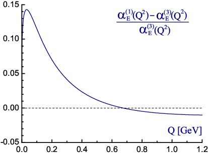
according to the world average. As displayed in Fig. 3.2, the relative difference
between the two curves is no more than 1 in the region of momentum transfer
GeV, to which the bulk of the states used as an input
in the calculation belongs.
Furthermore, as already noted, the set of equations (3.3-3.5) refer to a single definite quark-antiquark channels. So, having correct relativistic kinematics, they do not include coupling with other channels like any potential model (see App. A). Therefore, one can not expect to have any insight into the splitting of over-threshold complicated multiplets which involve mixture of different states. Even the position of the c.o.g. mass is expected to be reproduced only within one-half of the width of the state. This has been taken into account in the estimate of the theoretical error (see Sec. 4).
The resolution method of the eigenvalue equation for the operator (3.2, 3.3-3.5) used in [94, 95] and in the present work can be summarized as follows.
a) In the static limit the problem can be reduced to the corresponding one for the center of mass Hamiltonian (see App. A)
| (3.6) |
b) The eigenvalue equation for (3.6) is solved for a convenient fixed by the Rayleigh-Ritz method, using the three dimensional harmonic oscillator basis and diagonalizing a matrix.
c) The square of the meson mass is evaluated as , being the eigenfunction obtained in step b) (with the whole set of quantum numbers) and the operator given by Eq. (3.2).
d) Prescription c) is equivalent to treat as a first order perturbation. Consistently the hyperfine separation should be given by
| (3.7) |
where is the radial part of the complete eigenfunction
.
For the quark masses and string tension in (3.6)
the same values listed above have been used, and as far as
is concerned, that is supposed to be a constant
in (3.6), the value has been used, which is
the one typically used in non-relativistic calculations, and is also the
freezing value adopted in [94].
3.3 Extracting from the data
One focus now on the reversed problem, i.e., the determination
of the values at the characteristic
scales of a selected number of ground and excited states.
In order to estimate at low energy
one needs first to assign an effective -value to each state.
To this end one first rewrites the squared mass, as given by point c)
in Sec. 3.2, more explicitly as the sum of the unperturbed part, the
perturbative and the confinement ones respectively
| (3.8) |
Here is given by the second line of (3.3) and by Eq. (3.4) and the first two lines of (3.5). From the OGE contribution one then extracts for each state the fixed coupling value that leads to the same theoretical mass as by using given by Eq. (2.6). This can be done by means of the relation
| (3.9) |
where can be drawn again by the second line of Eq. (3.3). The effective momentum transfer associated to each bound state is then identified by the equation
| (3.10) |
The next step is to search for the correct (fixed) value of the coupling that exactly reproduces the experimental mass of each state. This is defined by the relation
| (3.11) |
so that, by combining Eqs. (3.8), (3.9) and (3.11) one finally obtains
| (3.12) |
This procedure has been applied to a number of light-light, light-heavy and heavy-heavy ground as well as excited states.
Before discussing the uncertainties related to the extracted
, few comments are in order.
First note that in the evaluation of in (3.9)
the hyperfine splitting has been neglected, whereas it has been taken
into account in (3.12), bringing possibly to different values of
for the singlet and the triplet states
(when there are reliable data for both).
Furthermore, the sensitivity of the effective ’s derived as above
from the specific coupling (2.6), has been
checked by analyzing their deviation for a shift of
around the value 193 MeV, and one finds
that the average change in the momentum scale amounts to .
This makes the resulting
reliable, at least qualitatively, even in
the deep IR region (GeV), where the discrepancy with respect
to massless is sizable.
Obviously the theoretical meson masses are sensitive to a variation
of the quark mass parameters (particularly in the case of the meson),
whereas and the relative
turn out to be much more stable. For instance, in the
light-light sector, an increase in the light quark mass of 5 amounts to
a change of about
in the value of and in the relative
.
Finally, a subtle point concerns the choice of
the “unperturbed” involved in the static
Hamiltonian (3.6). Actually, the value adopted is very near
to the pertaining to the state,
but definitively smaller than the typical
’s.
The point is that the hyperfine splitting is much
more sensible than the c.o.g. mass to the behaviour of the unperturbed
wave function at small distance (large momentum), which is specifically
controlled by the value of the unperturbed . As a result,
the effective fixed value in
Eq. (3.6) that reproduces the same splitting as by using the coupling
turns out to
be significantly smaller than calculated from
the c.o.g. mass. Essentially, it was chosen a phenomenological value
for the unperturbed in order to have a good reproduction
of the hyperfine splitting so as to reasonably reconstruct the
c.o.g. of the doublet when one component is missing. It was then used
the position of the c.o.g. (which is rather stable w.r.t. the unperturbed ) to extract the final result
.
3.4 Theoretical uncertainties
First of all, it should be clearly addressed the unavoidable model dependence of the
above results. Indeed, the formalism
exploited in their derivation is based on the
ansatz (3.1), consisting of
the sum of two contributions that one knows to be asymptotically correct for
small and large quark-antiquark distances. More sophisticated ansatz also
exist (see e.g. [91], [92] or
[93]), but they turn out to be difficult to implement
within BS formalism.
In the context of the model in hand the sources of error are the istantaneous
approximation implied by the three-dimensional reduction
of the BS equation, the approximations introduced into the resolution of
the eigenvalue equation, the inclusion of only the leading perturbative
contribution in the BS kernel , and finally having neglected the coupling
between different
quark antiquark channels.
Thus, aside from minor effects due to approximations in the resolution
of the eigenvalue equation and from the three-dimensional reduction, the main
sources of theoretical error in the
whole procedure are expected to arise from neglecting the NLO
contribution to the BS kernel as well as the coupling with other
channels, and these have been explicitly estimates.

The NLO contribution to the perturbative part of the BS-kernel comes from four diagrams with two-gluon exchange; two triangular graphs containing a four-line vertex of the type and two three-line vertices (the spin independent part of the second order BS formalism is quite similar to scalar QED), one fish diagram with two four-line vertices, and a crossing box with four three line vertices (see Fig. 3.3). If the renormalization scale is identified with the momentum transfer the fish graphs contribution is completely reabsorbed in the renormalization. On the other hand, a somewhat crude estimate of the contribution of each of the two triangular graphs yields
| (3.13) |
and for the crossing box graph, similarly
| (3.14) |
These expressions have to be compared with the leading one-gluon term used in the present calculation
| (3.15) |
Putting all things together, the overall error due to the omission of such NLO contributions to the BS kernel is then
| (3.16) |
and this produces
| (3.17) |
By using Eqs. (3.9-3.12), after some algebra it is easy to recognize that the NLO effects on turn out to be of the same order, that is
| (3.18) |
which is what is assumed in the foregoing.
The NLO errors do not exceed for heavy
quark states whereas they are enhanced up to when light and
strange quarks are involved.
Finally, since the strength of the neglected coupling with other
channels (OC) is obviously measured by the width of
the state, one roughly estimates an error of the order of in the evaluation of the theoretical meson mass . On this
basis, for each determination of
the related theoretical error is given by
| (3.19) |
Usually the error on the experimental mass is much smaller than . When, however, this is not the case one has to consider also the experimental error , obtained from (3.19) by replacing with .
All other sources of uncertainties aformentioned, that is, the errors implied by the three dimensional reduction, and by the approximations introduced in the resolution of the eigenvalue equation for , and the one due to the model dependence, though difficult to be explicitly estimated, can be globally taken into account by means of a comparison between the calculated and the experimental spectrum. To this aim, one can restrict the considerations to a sample of better established data which exclude high orbital excitations (D and F states), and introduce an additional conventional error on all the theoretical masses, defined by
| (3.20) |
where is the total error resulting from all the sources explicitly evaluated, i.e., , and the sum is restricted to the selected sample of data (namely, S and P states only). It turns out MeV, and then it can be set . This uncertainty, that turns out to be about on average, has not been included in the tables, but is used in the analysis of the following section.
3.5 BS-model results: concert of low and high energy data via APT
All results are displayed in details in tables I-VII of App. B, and
pictorially in Fig. 3.4. The first three columns specify the
state and its experimental mass as given by [2]. The fourth
column gives theoretical results for the meson masses, and the
last three give the effective ’s, the relative 3-loop APT coupling
and the experimental coupling with errors (both
theoretical and experimental).
In Fig. 3.4 values of at the same Q
from triplet and singlet states have been combined through a weighted
average according to their errors.
As one may infer from Fig. 3.4, the experimental points exhibit
a remarkable evolution from 500 MeV down to 200 MeV, where only the
safer S and P states are involved, in good agreement with the 3-loop
analytic coupling properly normalized,
i.e., with MeV, and discussed in Sec. 2
(cf. Eqs. (2.18) and (2.16), (2.17)).
Specifically, defining
as the total error explicitly evaluated
by means of Eqs. (3.18) and (3.19), one finds
| (3.21) |
The agreement quantitatively supports the relevance of the APT approach to IR phenomena down to a few hundred MeV.
On the other hand, at energies below 200 MeV there seems to exist a general tendency of
to deviate from the APT curve and to
approach zero, or at least a finite limit, which is less than the
universal APT freezing value. Note, however, that the analysis of
such an extreme IR behaviour is based on high orbital excitations (D
and F states), that lie well above the strong decay thresholds and
possess large widths. As a consequence, the theoretical reliability
of the method is lower at these scales, as apparent from the large
estimated errors. Moreover, also the discrepancy between (used in the calculation) and (used as a reference term) rises above 10 at these
scales. In fact, only two states (1670) (interpreted as ) and (2150) (), corresponding to
MeV, generate
(marginally) out of the error bands, and the state (2150), which
has been observed only once, has never been confirmed.
Nevertheless, as already noted, such a deep IR behaviour could
correlate with some lattice results [17], and could be
discussed within theoretical models, in particular within the recently developed
“massive” modification of APT, briefly
discussed in Sec. 2.4. Specifically, as displayed
in Fig. 3.4, the 1-loop coupling (2.34) with an effective mass MeV reasonably fits all experimental points down to the deep
infrared region.

Notice that in the selection of states irregular and incomplete multiplets have been excluded as a rule. Of this type, e.g., in the light quark sector, are the states ( is anomalously large and about twice as ), ( being larger than ), , , , (incomplete). If however included in the analysis, all these states would bring the results in agreement with the general tendency outlined.
As far as the renormalization scheme dependence is concerned, note that
the coupling definition is implicitly embodied in ansatz (3.1).
Specifically, here one assumes that after the area term subtraction,
is dominated by the OGE term, with the fixed
coupling replaced by the running coupling .
This amounts to including all the dressing effects into .
It is
worth noting that the coupling defined in such way is free of
unphysical singularities by construction.
At the same time, the 1-loop effective APT coupling
, involved in the calculation of the meson spectrum, is remarkably
stable with respect to both the higher loop corrections and the
choice of renormalization scheme (see Sec. 2. and a detailed
discussion of this issue in Ref. [63]). Thus one might expect that
the same situation should also occur for , with the possible
exception for the deep infrared region, where other
nonperturbative effects could be relevant.
Quark self-energy effects have been taken into account by a recursive
resolution of the Dyson-Schwinger equation. In the second order BS
formalism this simply amounts to replacing the current quark masses with
the constituent masses [95].

Finally, Fig. 3.5 displays a synthesis of the results for extracted from the bound states calculation in the BS framework, with a sample of high energy data as given by S. Bethke [1], against the 3-loop APT coupling (2.5) and its massive modification (2.34). Also shown in the figure is the common perturbative 3-loop coupling with IR singular behaviour that is ruled out by the data. As can be seen, the BS-APT theoretical scheme allows a rather satisfactory correlated understanding of very high and rather low energy phenomena.
Chapter 4 Conclusive remarks
To summarize, as discussed in Sec. 1, straightforward application
of the RG method to perturbative expansions in QCD eventually
gives rise to unphysical singularities in both the running coupling
and the physical observables, in the low energy domain. The Landau singularities
severely complicate theoretical analyses of hadron dynamics.
Then, an useful prescription to eliminate unphysical singularities is
provided by the APT approach, outlined in Sec. 2, which is
based upon the analycity requirement of the QCD coupling.
This prescription has been used in previous works in the framework
of a Bethe-Salpeter like formalism to compute the meson spectrum.
In this work, the point of view has been then somewhat reversed,
namely, as discussed in Sec. 3, the comparison between the
calculated meson spectrum within the BS framework and the experimental
data is used, in order to extract information on the infrared behavior
of the QCD running coupling.
The method consists in solving the eigenvalue equation for the
squared mass operator as given by Eq. (3.2), obtained by a
three dimensional reduction of the original BS equation. The
relativistic potential then follows from a proper
ansatz (3.1) on the Wilson loop to encode confinement,
and is the sum (3.2) of a one-gluon-exchange term and a confining term . The strong coupling occurring
in the perturbative part of the potential needs to be IR finite since
its argument has to be identified with the momentum transfer in the
interaction, and this typically takes values down to few
hundreds MeV.
As a first step, the common perturbative running coupling
has then been replaced by its 1-loop analytized
counterpart Eq. (2.6) as derived by the
APT algorithm, which avoids the hurdle of the spurious singularities in the
IR region [23], the whole theoretical scheme being
extensively discussed in Sec. 2.
An effective QCD scale MeV
has been imposed in order to reasonably reproduces the 3-loop APT coupling,
normalized at the Z boson mass along with world average [2] (i.e.,
MeV and MeV by
continuous threshold matching), specifically in the neighbohood of 0.5 GeV,
which is the typical scale of most of the imput states.
Then, it has been taken advantage of the BS results for the meson
spectrum, both in the light and heavy quark sector, to deduce within
this framework the fixed coupling value for each state that exactly
matches the theoretical and experimental mass.
A key point is finally the comparison of such experimental determinations
with the “Euclidean” APT coupling
and its further “massive” development.
The results are twofold. On the one hand, as expected on the basis of
the reasonable agreement between the theoretical and the experimental meson data, the 3-loop
analytic coupling remarkably fits the extracted points
from 1 GeV down to 200 MeV, within the evaluated errors, both theoretical and
experimental. This confirms and
yields a quantitative estimate of the relevance of the APT
to IR phenomena down to 200 MeV.
Besides, below this scale, the experimental points
exhibit a tendency to deviate with respect to the APT curve.
Despite the sizable errors, this could give a hint
on the vanishing of as in
concert with some results from lattice simulations [17].
It should be emphasized, however, that the existence of a finite IR limit
of , lower than the universal APT freezing value,
can not be ruled out by these data.
Neverthless, a vanishing QCD coupling at zero momentum transfer
can be theoretically discussed in the framework of a recent “massive”
modification [90] of the APT formalism, which takes into account
effects of a finite threshold in the dispersion relations. Since in the
extremely low region confinement forces play the dominant role, the
overall reasonable agreement between the “massive” APT model and the
results of the BS formalism would suggest a relation between the linear
potential, arising from the area term in the ansatz (3.1),
and the thresholds effects in the analytic properties of the QCD coupling,
that needs to be further investigated.
Appendix A: Second order Bethe-Salpeter formalism
In the QCD framework a second order four point quark-antiquark function and the full quark propagator can be defined as
| (4.1) |
and
| (4.2) |
where
| (4.3) |
and is the second order quark propagator in an external gauge field.
The quantity is defined by the second order differential equation
| (4.4) |
( and ) and it is related to the corresponding first order propagator by , being the so-called current mass of the quark.
The advantage of considering second order quantities is that the spin terms are more clearly separated and it is possible to write for a generalized Feynman-Schwinger representation, i.e., to solve Eq. (4.4) in terms of a quark path integral [24, 94]. Using the latter in (4.1) or (4.2) a similar representation can be obtained for and .
The interesting aspect of this final representation is that the gauge field appears in it only through a Wilson line correlator . In the limit , or the Wilson lines close in a single Wilson loop and if stays on a plane, can be written according to (3.1) as
| (4.5) | |||
The area term here is written as the algebraic sum of successive equal time strips and denotes the transversal component of . The basic assumption now is that, in the center of mass frame, (4.5) remains a good approximation even in the general case, i.e., for non flat curves and when , or . Then, by appropriate manipulations on the resulting expressions, an inhomogeneous Bethe-Salpeter equation for the 4-point function and a Dyson-Schwinger equation for can be derived in a kind of generalized ladder and rainbow approximation respectively. This should appear plausible, even from the point of view of graph resummation, for the analogy between the perturbative and the confinement terms in (4.5). In momentum representation, the corresponding homogeneous BS-equation becomes
| (4.6) | |||||
where ; ; the c.m. frame has to be understood, ; denotes the appropriate second order wave function, that in terms of the second order field can be defined as the Fourier transform of .
Similarly, in terms of the irreducible self-energy, defined by , the Dyson-Schwinger equation can be written
| (4.7) |
The kernels are the same in the two Eqs. (4.6) and (4.7), consistently with the requirement of chiral symmetry limit [25], being given by
| (4.8) |
where in the second and in the third equation has to be
understood. Notice that, due to the privileged role given to the c.m. frame,
the terms proportional to in (4.8) formally are not
covariant.
In fact, it can be checked that can
be consistently assumed to be spin independent and
Eq. (4.7) can be rewritten in the simpler form
| (4.9) |
with
| (4.10) | |||||
and denoting as above the transversal part of and . Eq. (4.9) can be solved by iteration resulting in an expression of the form , since (4.10) is not formally covariant. Then the constituent (pole) mass is defined by the equation
| (4.11) |
and the dependence on , being an artifact of the ansatz (3.1), is eliminated by extremizing in .
The 3-dimensional reduction of Eq. (4.6) can be obtained by a usual procedure of replacing with and with its so-called instantaneous approximation . In this way, one can explicitly integrate over and arrive to a 3-dimensional equation in the form of the eigenvalue equation for a squared mass operator Eq. (3.2), with [24]
| (4.12) |
Alternatively, in more usual terms, one could look for the eigenvalue of the mass operator or center of mass Hamiltonian with defined by . Neglecting term the linear form potential can be obtained from by the replacement . The resulting expression is particularly useful for a comparison with models based on potential. In particular, in the static limit reduces to the Cornell potential
| (4.13) |
Note that it is necessary to introduce a cut-off in Eq. (4.9). As a consequence the constituent mass turns out to be a function of the current mass and of , . Then if one uses a running current mass , a running constituent mass is obtained, as it has been done in [95]. However the singular expression used there
| (4.14) |
is not consistent with Eq. (2.6), and if a more consistent assumption is taken, e.g.,
| (4.15) |
or the other resulting from the analytization of a similar expression with replaced with the ordinary perturbative , the dependence of on is strongly reduced. For this reason even the light quark mass is here treated as a constants to be adjusted with the the data11 1 In this way the only role that is left to the DS equation is to justify the difference between the constituent and the current masses..
Appendix B: Numerical results
The tables below display the complete set of results as explained in
Sec. 3.5. The values of all the parameters are
, , ,
, and
. Meson masses are given in MeV. The last
column displays the experimental coupling with the theoretical error due to
the next-to-leading order terms neglected, the
theoretical error from the half width and the experimental error
respectively.
† Center of gravity masses of the incomplete
multiplets estimated in analogy with other multiplets.
| States | (MeV) | |||||
|---|---|---|---|---|---|---|
| 136 | 401 | 0.522 | ||||
| 775.5 0.4 | 749 | |||||
| 638 | 613 | |||||
| 1300 100 | 1223 | 448 | 0.502 | |||
| 1459 11 | 1363 | |||||
| 159 | 139 | |||||
| 1229.5 3.2 | 1234 | 209 | 0.637 | |||
| 1595 | 144 | 0.701 |
| States | (MeV) | |||||
| 1019.460 0.019 | 1019 | 418 | 0.514 | |||
| 1680 20 | 1602 | 454 | 0.500 | |||
| 1386 19 | 1472 | 216 | 0.631 | |||
| 1484 | ||||||
| 1807 | 149 | 0.695 | ||||
| 2070 | 118 | 0.733 |
| States | (MeV) | |||||
| 491 | 409 | 0.518 | ||||
| 887 | ||||||
| 398 | 396 | |||||
| 1414 15 | 1485 | 451 | 0.501 | |||
| 1272 7 | 1355 | 213 | 0.634 | |||
| 1367 | ||||||
| 1712 | 150 | 0.694 | ||||
| 1973 | 116 | 0.736 |
| States | (MeV) | |||||
| 2980.4 1.2 | 2980 | 561 | 0.464 | |||
| 3096.916 0.011 | 3097 | |||||
| 117 | 118 | |||||
| 3638 4 | 3595 | 500 | 0.483 | |||
| 3686.093 0.034 | 3653 | |||||
| 48 | 58 | |||||
| 4039 1 | 4030 | 483 | 0.489 | |||
| 4421 4 | 4337 | 474 | 0.492 | |||
| 3525.93 0.27 | 3532 | 269 | 0.592 | |||
| 3537 | ||||||
| 3929 | 274 | 0.589 | ||||
| 3822 | 190 | 0.654 | ||||
| 4150 | 198 | 0.646 |
Quantum numbers of and mesons are not well established.
| States | (MeV) | |||||
| 9460.30 0.26 | 9461 | 951 | 0.381 | |||
| 10023.26 0.31 | 9987 | 630 | 0.445 | |||
| 10355.2 0.5 | 10321 | 552 | 0.466 | |||
| 10579.4 1.2 | 10588 | 517 | 0.478 | |||
| 10865 8 | 10820 | 497 | 0.484 | |||
| 11019 8 | 11034 | 506 | 0.481 | |||
| 9880 | 387 | 0.528 | ||||
| 10231 | 343 | 0.549 |
| States | (MeV) | |||||
| 1843 | 459 | 0.498 | ||||
| 2000 | ||||||
| 141 1 | 157 | |||||
| 2443 | 232 | 0.619 | ||||
| 5246 | 516 | 0.478 | ||||
| 5325.0 0.6 | 5311 | |||||
| 46 3 | 64 |
| States | (MeV) | |||||
| 1968.2 0.5 | 1959 | 472 | 0.493 | |||
| 2112.0 0.6 | 2109 | |||||
| 144 1 | 149 | |||||
| 2545 | 236 | 0.616 | ||||
| 5367.5 1.8 | 5343 | 535 | 0.472 | |||
| 5412.8 1.7 | 5408 | |||||
| 47 4 | 65 | |||||
| 5853 15 | 5830 | 255 | 0.602 |
Bibliography
- [1] S. Bethke, Prog. Part. Nucl. Phys. 58, 351 (2007) [arXiv:hep-ex/0606035]; Nucl. Phys. Proc. Suppl. 135 (2004) 345; 121 (2003) 74; J. Phys. G 26 (2000) R27.
- [2] S. Eidelman et al. [Particle Data Group], Phys. Lett. B 592 (2004) 1.
- [3] M. Baldicchi, A. V. Nesterenko, G. M. Prosperi, D. V. Shirkov and C. Simolo, Phys. Rev. Lett. 99 (2007) 242001 [arXiv:0705.0329 [hep-ph]].
- [4] M. Baldicchi, A. V. Nesterenko, G. M. Prosperi and C. Simolo, arXiv:0705.1695 [hep-ph], to appear on Phys. Rev. D.
- [5] D. V. Shirkov, V. F. Kovalev, Phys. Rept. 352, 219 (2001).
- [6] G. M. Prosperi, M. Raciti and C. Simolo, Prog. Part. Nucl. Phys. 58 (2007) 387 [arXiv:hep-ph/0607209].
- [7] S. J. Brodsky, G. P. Lepage and P. B. Mackenzie, Phys. Rev. D 28 (1983) 228; S. J. Brodsky, C. R. Ji, A. Pang and D. G. Robertson, Phys. Rev. D 57 (1998) 245; G. Grunberg, Phys. Rev. D 46 (1992) 2228.
- [8] S. Ciulli and J. Fischer, Nucl. Phys. 24, 465 (1961); J. Fischer, Fortschr. Phys. 42, 665 (1994); I. Caprini and J. Fischer, Phys. Rev. D 60, 054014 (1999); 62, 054007 (2000); 68, 114010 (2003); 71, 094017 (2005); arXiv:hep-ph/0612274.
- [9] D.M. Howe and C.J. Maxwell, Phys. Rev. D 70, 014002 (2004); P.M. Brooks and C.J. Maxwell, ibid. D 74, 065012 (2006); C.J. Maxwell, arXiv:hep-ph/0610183.
- [10] G. Grunberg, Phys. Rev. D 29 (1984) 2315; Phys. Lett. B 95 (1980) 70 [Erratum-ibid. B 110 (1982) 501]; Phys. Rev. D 40 (1989) 680.
- [11] Yu. L. Dokshitzer, G. Marchesini and B. R. Webber, Nucl. Phys. B 469 (1996) 93.
- [12] S. J. Brodsky, S. Menke, C. Merino and J. Ratsham, Phys. Rev. D 67 (2003) 055008 and references therein.
- [13] (ALEPH Collaboration), R. Barate et al. Eur. Phys. J. C 4 (1998) 409; (OPAL Collaboration), K. Ackerstaff et al. Eur. Phys. J. C 7 (1999) 571. E. Braaten, S. Narison and A. Pich, Nucl. Phys. B 373 (1992) 581.
- [14] A. C. Mattingly and P. M. Stevenson, Phys. Rev. D 49 (1994) 437; P. M. Stevenson, Phys. Rev. D 23 (1981) 2916; Nucl. Phys. B 231 (1984) 65; J. Kubo, S. Sakakibara, and P. M. Stevenson, Phys. Rev. D 29 (1984) 1682; A. C. Mattingly and P. M. Stevenson, Phys. Rev. Lett. 69 (1992) 1320.
- [15] A. L. Kataev, S. A. Larin, and L. R. Surguladze, Phys. Rev. D 43 (1991) 1633; J. Chýla, A. Kataev, and S. Larin, Phys. Lett. B 267 (1991) 269.
- [16] D.V. Shirkov, Teor. Mat. Fiz. 136, 3 (2003) [Theor. Math. Phys. 136, 893 (2003)].
- [17] R. Alkofer and L. von Smekal, Phys. Rept. 353, 281 (2001); P. Boucaud et al., Nucl. Phys. Proc. Suppl. 106, 266 (2002); J. Skullerud, A. Kizilersu, and A.G. Williams, Nucl. Phys. Proc. Suppl. 106, 841 (2002).
- [18] J. L, Richardson, Phys. Lett. B 82 (1979) 272.
- [19] W. Buchmüller, G. Grunberg and S.-H. H. Tye, Phys. Rev. Lett. 45 (1980) 103; Phys. Rev. Lett. 45 (1980) 587; W. Fischler, Nucl. Phys. B 129 (1977) 157; A. Billoire, Phys. Lett. B 92 (1980) 343; M. Peter, Phys. Rev. Lett. 78 (1997) 602; Y. Schroder, Phys. Lett. B 447 (1999) 321.
- [20] E. Eichten and F. Feinberg, Phys. Rev. D 23 (1989) 2724; N. Brambilla, P. Consoli and G. M. Prosperi, Phys. Rev. D 50 (1994) 5878; Yu. A. Simonov, Nucl. Phys. B 324 (1989) 67.
- [21] S. Godfrey and N. Isgur, Phys. Rev. D 32 (1985) 189; T. Barnes, F. E. Close and S. Monaghan, Nucl. Phys. B 198 (1983) 380; G. M. Prosperi and M. Baldicchi, Fizika B 8 (1999) 251; T. Zhang and R. Koniuk, Phys. Lett. B 261 (1991) 311.
- [22] P. Ball, M. Beneke and V. M. Braun, Nucl. Phys. B 452 (1995) 563; J. Papavassiliou and J. M. Cornwall, Phys. Rev. D 44 (1991) 1285; J. H. Field, Phys. Rev. D 66 (2002) 013013;
- [23] D.V. Shirkov and I.L. Solovtsov, JINR Rapid Comm. 2, 5 (1996); arXiv:hep-ph/9604363; Phys. Rev. Lett. 79, 1209 (1997).
- [24] N. Brambilla, E. Montaldi, and G.M. Prosperi, Phys. Rev. D 54, 3506 (1996); G.M. Prosperi, Problems of Quantum Theory of Fields, p. 381, B.M. Barbashov, G.V. Efimov, A.V. Efremov Eds. JINR Dubna 1999, arXiv:hep-ph/9906237.
- [25] M. B. Hecht, C. D. Roberts and S. M. Schmidt, Phys. Rev. C 63 (2001) 025213
- [26] F. Jugeau and H. Sazdjian, Nucl. Phys. B 670 (2003) 221; J. Mourad and H. Sazdjian, J. Phys. G 21 (1995) 267; J. Math. Phys. 35 (1994) 6379.
- [27] A. M. Badalian, B. L. G. Bakker and Yu. A. Simonov, Phys. Rev. D 75 (2007) 116001; A. M. Badalian and D. S. Kuzmenko, Phys. Rev. D 65 (2002) 016004.
- [28] D. Ebert, R. N. Faustov and V. O. Galkin, Mod. Phys. Lett. A 20 (2005) 1887; Eur. Phys. J. C 47 (2006) 745.
- [29] T. van Ritbergen, J. A. M. Vermaseren and S. A. Larin, Phys. Lett. B 400 (1997) 379.
- [30] W. E. Caswell and F. Wilczek, Phys. Lett. B 49 (1974) 291.
- [31] D. J. Gross and F. Wilczek, Phys. Rev. Lett. 30 (1973) 1343.
- [32] W. E. Caswell, Phys. Rev. Lett. 33 (1974) 244; D. R. T. Jones, Nucl. Phys. B 75 (1974) 531.
- [33] O. V. Tarasov, A. A. Vladimirov and A. Y. Zharkov, Phys. Lett. B 93 (1980) 429.
- [34] S. A. Larin and J. A. M. Vermaseren, Phys. Lett. B 303 (1993) 334.
- [35] M. Czakon, Nucl. Phys. B 710 (2005) 485; T. R. Morris and O. J. Rosten, arXiv:hep-th/0606189.
- [36] W. A. Bardeen, A. J. Buras, D. W. Duke and T. Muta, Phys. Rev. D 18 (1978) 3998.
- [37] J. C. Collins, Renormalization, Cambridge University Press (1984).
- [38] R. M. Corless, G. H. Gonnet, D. E. G. Hare, D. J. Jeffrey, and D. E. Knuth, Advances in Computation Mathematics, V 5 (1996) 329.
- [39] E. Gardi, G. Grunberg and M. Karliner, JHEP 9807 (1998) 007.
- [40] K. G. Chetyrkin, B. A. Kniehl and M. Steinhauser, Phys. Rev. Lett. 79 (1997) 2184.
- [41] D. S. Kourashev, arXiv:hep-ph/9912410.
- [42] D. S. Kurashev and B. A. Magradze, Theor. Math. Phys. 135 (2003) 531 [Teor. Mat. Fiz. 135 (2003) 95]; B. A. Magradze, arXiv:hep-ph/0305020.
- [43] B. A. Magradze, Few Body Syst. 40, 71 (2006); arXiv:hep-ph/0512374.
- [44] A. V. Radyushkin, JINR Rapid Commun. 78 (1996) 96 [arXiv:hep-ph/9907228].
- [45] W. Celmaster and R. J. Gonsalves, Phys. Rev. D 20 (1979) 1420.
- [46] W. Bernreuther, A. Brandenburg and P. Uwer, Phys. Rev. Lett. 79 (1997) 189; K. G. Chetyrkin and J. H. Kuhn, Phys. Lett. B 406 (1997) 102.
- [47] J. A. M. Vermaseren, S. A. Larin and T. van Ritbergen, Phys. Lett. B 405 (1997) 327; K. G. Chetyrkin and A. Retey, Nucl. Phys. B 583 (2000) 3.
- [48] K. Melnikov and T. v. Ritbergen, Phys. Lett. B 482 (2000) 99.
- [49] S. A. Larin, T. van Ritbergen and J. A. M. Vermaseren, Nucl. Phys. B 438 (1995) 278; K. G. Chetyrkin, B. A. Kniehl and M. Steinhauser, Nucl. Phys. B 510 (1998) 61; G. Rodrigo, A. Pich and A. Santamaria, Phys. Lett. B 424 (1998) 367; G. Rodrigo and A. Santamaria, Phys. Lett. B 313 (1993) 441.
- [50] D. V. Shirkov, Nucl. Phys. B 371 (1992) 467; D. V. Shirkov and S. V. Mikhailov, Z. Phys. C 63 (1994) 463.
- [51] R. G. Moorhouse, M. R. Pennington and G. G. Ross, Nucl. Phys. B 124 (1977) 285.
- [52] S. L. Adler, Phys. Rev. D 10 (1974) 3714.
- [53] K. G. Chetyrkin, A. L. Kataev and F. V. Tkachov, Phys. Lett. B 85 (1979) 277; W. Celmaster, R. J. Gonsalves, Phys. Rev. Lett. 44 (1980) 560; M. Dine, J. R. Sapirstein, Phys. Rev. Lett. 43 (1979) 668; S. G. Gorishnii, A. L. Kataev and S. A. Larin, Phys. Lett. B 259 (1991) 144; L. R. Surguladze and M. A. Samuel, Phys. Rev. Lett. 66 (1991) 560 [Erratum-ibid. 66 (1991) 2416].
- [54] A. L. Kataev and V. V. Starshenko, Mod. Phys. Lett. A 10 (1995) 235.
- [55] J. D. Bjorken, SLAC-PUB-5103 Invited lectures given at 1989 Cargese Summer Inst. in Particle Physics, Cargese, France, Jul 18 - Aug 4, 1989.
- [56] M. R. Pennington and G. G. Ross, Phys. Lett. B 102 (1981) 167.
- [57] M. R. Pennington, R. G. Roberts and G. G. Ross, Nucl. Phys. B 242 (1984) 69.
- [58] N. V. Krasnikov and A. A. Pivovarov, Phys. Lett. B 116 (1982) 168.
- [59] H. F. Jones and I. L. Solovtsov, Phys. Lett. B 349 (1995) 519.
- [60] P.J. Redmond, Phys. Rev. 112, 1404 (1958); P.J. Redmond and J.L. Uretsky, Phys. Rev. Lett. 1, 147 (1958); N.N. Bogoliubov, A.A. Logunov, and D.V. Shirkov, Zh. Eksp. Teor. Fiz. 37, 805 (1959) [Sov. Phys. JETP 37, 574 (1960)].
- [61] D.V. Shirkov and I.L. Solovtsov, Phys. Lett. B 442, 344 (1998); arXiv:hep-ph/9711251; Teor. Mat. Fiz. 120, 482 (1999) [Theor. Math. Phys. 120, 1220 (1999)]; arXiv:hep-ph/9909305.
- [62] K.A. Milton and I.L. Solovtsov, Phys. Rev. D 55, 5295 (1997); 59, 107701 (1999).
- [63] D.V. Shirkov and I.L. Solovtsov, Theor. Math. Phys. 150, 132 (2007); arXiv:hep-ph/0611229.
- [64] A.P. Bakulev, S.V. Mikhailov and N.G. Stefanis, Phys. Rev. D 75, 056005 (2007); arXiv:hep-ph/0607040.
- [65] D.V. Shirkov, Teor. Mat. Fiz. 119, 55 (1999) [Theor. Math. Phys. 119, 438 (1999)]; arXiv:hep-th/9810246; Lett. Math. Phys. 48, 135 (1999).
- [66] B. A. Magradze, Int. J. Mod. Phys. A 15 (2000) 2715; arXiv:hep-ph/9808247.
- [67] B. A. Magradze, arXiv:hep-ph/0010070.
- [68] K. A. Milton, I. L. Solovtsov and O. P. Solovtsova, Phys. Lett. B 415 (1997) 104.
- [69] A. I. Alekseev, Few Body Syst. 32 (2003) 193.
- [70] A. I. Alekseev, Phys. Rev. D 61 (2000) 114005; A. I. Alekseev, Phys. Atom. Nucl. 65 (2002) 1678 [Yad. Fiz. 65 (2002) 1722]; J. Phys. G 27 (2001) L117.
- [71] A.V. Nesterenko, Int. J. Mod. Phys. A 18, 5475 (2003); Int. J. Mod. Phys. A 19 (2004) 3471.
- [72] D.V. Shirkov and A.V. Zayakin, Yad. Fiz. 70, 808 (2007) [Phys. Atom. Nucl. 70, 775 (2007)]; arXiv:hep-ph/0512325.
- [73] A. P. Bakulev, K. Passek-Kumericki, W. Schroers and N. G. Stefanis, Phys. Rev. D 70 (2004) 033014 [Erratum-ibid. D 70 (2004) 079906].
- [74] K. A. Milton and O. P. Solovtsova, Phys. Rev. D 57 (1998) 5402; K. A. Milton and I. L. Solovtsov, Phys. Rev. D 55 (1997) 5295.
- [75] I. L. Solovtsov and D. V. Shirkov, Phys. Lett. B 442 (1998) 344.
- [76] D. V. Shirkov, Theor. Math. Phys. 127 (2001) 409; arXiv:hep-ph/0003242.
- [77] D. V. Shirkov, Eur. Phys. J. C 22 (2001) 331.
- [78] A. P. Bakulev, S. V. Mikhailov and N. G. Stefanis, Phys. Rev. D 75 (2007) 056005 [arXiv:hep-ph/0607040]; A. P. Bakulev, A. I. Karanikas and N. G. Stefanis, Phys. Rev. D 72 (2005) 074015.
- [79] J. S. Schwinger, Proc. Nat. Acad. Sci. 71, 5047 (1974); K. A. Milton, Phys. Rev. D 10 (1974) 4247.
- [80] K. A. Milton and I. L. Solovtsov, Phys. Rev. D 59 (1999) 107701.
- [81] K. A. Milton, I. L. Solovtsov and O. P. Solovtsova, Phys. Lett. B 439 (1998) 421; Phys. Rev. D 60 (1999) 016001; K. A. Milton, I. L. Solovtsov, O. P. Solovtsova and V. I. Yasnov, Eur. Phys. J. C 14 (2000) 495; K. A. Milton, I. L. Solovtsov and O. P. Solovtsova, Phys. Rev. D 64 (2001) 016005; O. P. Solovtsova, Theor. Math. Phys. 134 (2003) 365 [Teor. Mat. Fiz. 134 (2003) 416]; B. V. Geshkenbein, B. L. Ioffe and K. N. Zyablyuk, Phys. Rev. D 64 (2001) 093009.
- [82] D. V. Shirkov, Theor. Math. Phys. 136 (2003) 893 [Teor. Mat. Fiz. 136 (2003) 3]; D. V. Shirkov, arXiv:hep-ph/0408272.
- [83] G. Cvetic and C. Valenzuela, J. Phys. G 32, L27 (2006); Phys. Rev. D 74, 114030 (2006); G. Cvetic, C. Valenzuela, and I. Schmidt, Nucl. Phys. Proc. Suppl. 164, 308 (2007).
- [84] F. Schrempp, J. Phys. G 28 (2002) 915.
- [85] A. I. Alekseev and B. A. Arbuzov, Mod. Phys. Lett. A 20 (2005) 103; Mod. Phys. Lett. A 13 (1998) 1747; A. I. Alekseev, Theor. Math. Phys. 145 (2005) 1559 [Teor. Mat. Fiz. 145 (2005) 221]; Few Body Syst. 40, 57 (2006); arXiv:hep-ph/0503242.
- [86] A. V. Nesterenko and I. L. Solovtsov, Mod. Phys. Lett. A 16 (2001) 2517; A. V. Nesterenko, Phys. Rev. D 62 (2000) 094028.
- [87] P.A. Raczka, Nucl. Phys. Proc. Suppl. 164, 211 (2007); arXiv:hep-ph/0602085; arXiv:hep-ph/0608196.
- [88] N. V. Krasnikov and A. A. Pivovarov, Phys. Atom. Nucl. 64 (2001) 1500 [Yad. Fiz. 64 (2001) 1576].
- [89] B. R. Webber, JHEP 9810 (1998) 012.
- [90] A.V. Nesterenko and J. Papavassiliou, J. Phys. G 32, 1025 (2006); arXiv:hep-ph/0507320; A. C. Aguilar, A. V. Nesterenko and J. Papavassiliou, J. Phys. G 31 (2005) 997.
- [91] Y. Nambu, Phys. Lett. B 80 (1979) 372. For recent developments see e.g. H. G. Dosch, M. Luscher and P. Weisz, JHEP 0207 (2002) 049; M. Billo, M. Caselle and L. Ferro, JHEP 0602 (2006) 070, and references therein.
- [92] H. G. Dosch, Phys. Lett. B 190 (1987) 177; H. G. Dosch and Yu. A. Simonov, Phys. Lett. B 205 (1988) 339.
- [93] M. Baker, J. S. Ball and F. Zachariasen, Phys. Rev. D 51 (1995) 1968; M. Baker, J. S. Ball, N. Brambilla, G. M. Prosperi and F. Zachariasen, Phys. Rev. D 54 (1996) 2829 [Erratum-ibid. D 56 (1997) 2475]
- [94] M. Baldicchi and G.M. Prosperi, Phys. Rev. D 66, 074008 (2002); 62, 114024 (2000); Fizika B 8, 251 (1999); Phys. Lett. B 436, 145 (1998).
- [95] M. Baldicchi and G.M. Prosperi, AIP Conf. Proc. 756, 152 (2005); Color Confinement and Hadrons in Quantum Chromodynamics, p. 183, H. Suganuma, et al. eds. World Scientific 2004, arXiv:hep-ph/0310213.
- [96] M. Baldicchi, G.M. Prosperi, and C. Simolo, AIP Conf. Proc. 892 (2007) 340 [arXiv:hep-ph/0611087].
Part II Progress in the determination of the gluon polarization
Chapter 5 Polarized parton distributions from DIS
One of the fundamental properties of the nucleon structure is the
spin distribution among its quark and gluon constituents. The spin
structure of the nucleon has been extensively
investigated by inclusive polarized lepton scattering off polarized
protons and neutrons, since the discovery of the EMC spin
effect [1].
Despite the naive expectation that the nucleon spin is carried by quarks,
the experimental results revealed that only a small fraction is
actually due to quarks (the so-called “proton spin crisis”).
Considerable efforts, both experimentally and theoretically, have
subsequentely gone into understanding where the remaining fraction of
the nucleon spin resides (see e.g. Ref. [2] for a recent
review).
To this end, the determination of the first moments of the polarized
parton distribution functions (pdfs) is necessary.
Attention is currently devoted to the reconstruction of pdfs
at all values of the Bjorken and the momentum transfer . Of
special interest is the determination of the gluon polarization, in
order to evaluate the total contribution carried by the gluons to the nucleon
spin.
The possibility of inferring the polarized gluon density from scaling violations has been extensively studied. However, phenomenological analyses of the current inclusive DIS data only yield weak constraints on the gluon first moment, and leave the -shape completely undetermined. This issue has been thoroughly investigated in the present work, by performing a NLO analysis in perturbative QCD of world data from inclusive DIS experiments, as discussed in detail in Sec. 6.
Actually, some light may be shed on the gluon content of the nucleon by observing specific events that receive leading contributions from gluon initiated subprocesses, that is, by directly measuring the polarized gluon density. In particular, as discussed in Sec. 7, in polarized fixed target experiments, the gluon polarization can be probed through the photon-gluon fusion process, by selecting open-charm events or hadron pairs with high transverse momentum, and both strategies are currently used at the COMPASS experiment (CERN). Indeed charmed mesons in the final states provide a clean tag of photon-gluon fusion, since there are essentially no competing processes and a clean perturbative analysis is possible. Therefore, a phenomenological study of open-charm photoproduction from deep-inelastic muon scattering off nucleons, with longitudinally polarized beam and target, has been also performed, with reference to upcoming results on experimental asymmetries from COMPASS. The results are presented in Sec. 7 and, specifically, the constraints that can be obtained on the polarized gluon density at the COMPASS kinematics are discussed.
In what follows the main theoretical tools are briefly reviewed. Specifically Sec. 5.1 recalls the basic ingredients for the study of polarized lepton-nucleon scattering, i.e. the polarized structure functions and . In Sec. 5.2 the expectations of the naive quark-parton model are summarized, whereas Sec. 5.3 is devoted to the main aspects of the perturbative QCD analysis, that is, the relations between structure functions and polarized parton distributions. In Sec. 5.4 the way experimental information on the relevant structure function are extracted from the experimentally measured quantities is described, and, finally Sec 5.5 sketches how target mass corrections are taken into account in the present analysis.
5.1 Structure functions and their moments
Polarized structure functions are the form factors which parametrize the cross section for deep-inelastic scattering of polarized leptons off a polarized hadronic target. If the momentum transfer involved is much smaller than the boson mass, the antisymmetric part of the hadronic tensor can be expressed in terms of two spin-dependent structure functions, and , i.e. [3, 4]
| (5.1) |
where and are, respectively, the target four-momentum, mass, and spin (normalized as ). Neglecting weak interaction effects, in Eq. (5.1) is the electric current. The deeply inelastic region is identified by the Bjorken limit
| (5.2) |
in which the invariant mass of the hadronic system in the final state is much larger than the nucleon mass, namely
| (5.3) |
In the case when the nucleon spin is purely longitudinal, that is,
| (5.4) |
the antysimmetric tensor Eq. (5.1) can be written as
| (5.5) |
In the Bjorken limit the product , thus leaving a finite residue
as . Furthermore, the factor vanishes, and the structure
function decouples. As a result only is asimptotically relevant.
In case of transverse polarization both structure functions equally contribute,
but the whole cross section is strongly suppressed by an overall target mass
factor.
The light-cone expansion of the current product in Eq. (5.1) implies that the first moment of the relevant structure function for a nucleon target, at leading twist, is given by [5]
| (5.6) |
where are given by matrix elements of the axial current for the -th flavor, namely
| (5.7) |
is the electric charge, and are perturbatively calculable coefficient functions. Then, assuming that only the three lightest flavors are activated, Eq. (5.6) can be recast as
| (5.8) |
where the plus (minus) sign refers to a proton (neutron) target, and the singlet and nonsinglet matrix elements are defined by
| (5.9) |
respectively. and are -dependent singlet and nonsinglet QCD coefficient functions; to order , in the scheme e.g., one has
| (5.10) |
whereas at higher orders [6]. QCD
corrections turn out to be sizable in the -range of the present experiments
and are thus relevant for the comparison with the data [7].
The singlet and nonsinglet components of can be then extracted using
Eq. (5.8).
Indeed, the triplet and octet currents are conserved and therefore scale invariant,
and the related matrix elements can be derived from any other process.
The triplet axial charge is equal to the axial coupling measured in nucleon
-decay
| (5.11) |
where and are weak hyperon decay constants in flavor SU(3) symmetry [8, 9]. The octet matrix element is then given by
| (5.12) |
On the other hand, the singlet axial charge is scale dependent due to the anomalous nonconservation of the singlet axial current [10], and can be determined from a measurement of the proton first moment, by rewriting Eq. (5.8) as
| (5.13) |
Since the two terms on the right hand side are roughly of the same order (typically ), the value of arises from a large cancellation between them (see e.g. [4]). Present data indeed indicate that is compatible with zero, but values as large as are not excluded.
Finally, a fundamental prediction of the theory is the Bjorken sum rule
| (5.14) |
that was originally derived from current algebra and isospin symmetry [11]. Eq. (5.14) relates the integral over all of the nonsinglet polarized structure function , at fixed , to the well-measured -decay coupling . A comparison with the data, using the computed thus allows a direct test of isospin in this channel, as well as the predicted scale dependence. In addition, it is possible to use the measurements to extract a relatively accurate determination of the strong coupling [12].
5.2 The parton model predictions
In the naive quark-parton model the spin-dependent structure function can be simply expressed as the charge-weighted difference between momentum distributions for quark helicities aligned parallel and antiparallel to the longitudinally polarized parent nucleon
| (5.15) |
The polarized quark distributions are defined as
| (5.16) |
and similarly for antiquarks. Assuming , one can define the flavor singlet and nonsinglet combinations of polarized quark densities, namely
| (5.17) |
Then the structure function can be cast into the form
| (5.18) |
where the plus (minus) sign stays for a proton (neutron) target, and the
average charge is for .
In the naive parton model gluons do not contribute to the nucleon spin, and
the first moments of singlet and nonsinglet quark densities are
straightforwardly related to the matrix elements of axial currents, such
that
| (5.19) |
In this context, the first moments of can be interpreted
as the contribution of the quark flavor to the nucleon spin, and thus
the singlet axial charge as the net quark helicity.
Then, under the assumption
that the strange sea in the nucleon is unpolarized, namely
| (5.20) |
the quark helicity coincides with the nonsinglet (octet) axial charge, . Thus, from Eq. (5.12) one roughly has
| (5.21) |
whereas the value extracted from the data (see Eq. (5.13)) is compatible with zero. The Ellis-Jaffe sum rules [13] then give the parton model predictions for the proton and neutron first moments
| (5.22) |
that are not consistent with the measured values, at the level of several standard deviations. Thus, against the Ellis-Jaffe prediction and intuition, quarks seem to carry a very small fraction of the total nucleon helicity. Actually, it is only at the naive parton level that the first moment of the singlet part of the structure function corresponds to the total helicity fraction carried by quarks.
5.3 Polarized structure functions and pdfs in QCD
When including QCD corrections, also the gluon density contributes and the structure function is related to the scale-dependent polarized quark and gluon distributions by the convolution with appropriate coefficient functions [17, 18]
| (5.23) |
where , being the number of active flavors with electric charge , and denotes the convolution product with respect to
| (5.24) |
In Eq. (5.23) is the polarized gluon distribution, whereas the singlet and nonsinglet quark distributions are defined as
| (5.25) | |||
where and are the scale-dependent quark and antiquark polarized densities of flavor , defined as in Eq. (5.16).
The perturbative part of the -dependence of the polarized parton densities is given by the Altarelli-Parisi evolution equations [19]. The singlet quark and gluon distributions mix according to
| (5.26) |
while the nonsinglet quark evolves independently as
| (5.27) |
In Eqs. (5.26) and (5.27) denote the spin-dependent
splitting functions, and with the QCD scale
parameter. The factorization and renormalization
scales are both taken equal to , so that all the scale dependence appears
through .
Eqs. (5.26) and (5.27) are valid
for all orders of perturbative QCD; the coefficient functions and the
evolution kernels may each be expanded in
powers of . At NLO
| (5.28) |
| (5.29) |
It is also convenient to introduce anomalous dimensions
| (5.30) |
i.e. the Mellin transforms of the splitting functions. One can analogously
define moment-space coefficient functions and parton distributions
, and .
In accordance with the partonic picture, in Eq. (5.28)
, while , so that
at order decouples from , and
is just a linear combination of polarized quark distributions, whose dependence
is entirely specified by Eqs. (5.26) and (5.27) (the leading order
splitting functions are calculated in Ref. [19]).
Beyond leading order, splitting functions and coefficient functions are no
longer universal, hence even though the scale dependence of the observable
structure function is determined uniquely, at least up to higher order
corrections, its separation into contributions due to quarks and gluons is scheme
dependent and thus essentially arbitrary. The NLO coefficient functions may be
modified by a change of the factorization scheme which is partially compensated
by a corresponding change in the NLO anomalous dimensions, hence both are required
in a full NLO order computation. The complete set of NLO coefficient functions and
splitting functions can be found in Ref. [6].
The modified minimal subtraction () factorization scheme is
commonly used in the analysis of polarized parton distributions.
In the scheme
the first moment of the gluon coefficient function vanishes, the gluon density does not
contribute to the first moment of and the scale dependent singlet axial
charge is thus equal to the singlet quark first moment
| (5.31) |
Alternatively, one can define a different scheme, the Adler-Bardeen (AB) scheme [10], such that the singlet quark first moment is conserved at all orders and can be identified with the total quark helicity, whereas the polarized gluon density is defined as in the scheme. In the AB scheme the gluon polarization directly contributes to the singlet axial charge (and thus to the first moment of ), which is now written as
| (5.32) |
Eqs. (5.31) and (5.32) then yield the relation between the first moments of the singlet quark distributions in the two schemes. They differ by the product , which is due to the anomalous nonconservation of the singlet axial current [10], and is scale invariant at leading order; this implies that increases as with , and the gluon contribution in Eq. (5.32) is not asymptotically suppressed by powers of . As a result, this scheme dependence does not vanish at large , and the definition of the singlet quark first moment is therefore maximally ambiguous.
In the AB scheme, which will be adopted in the following phenomenological analysis (see Sec. 6), the first moment of the gluon coefficient function at NLO reads [10]
| (5.33) |
and the first moment of the structure function is given at NLO by
| (5.34) | |||
Different factorization schemes were also discussed in Refs. [20], and the dependence of the results of phenomenological analyses of spin-dependent pdfs on the choice of the scheme was studied.
It should be finally noted that a number of theoretical models attempt to
explain the quark helicity distribution
within the nucleon and the unexpected smallness of the singlet axial charge. A
possible interpretation is to assume a large and negative contribution from the
strange sea polarization . This suppression of the axial charge might
be explained by invoking nonperturbative mechanisms based on instanton-like vacuum
configuration [14]. In this case . Another scenario
is possible, where the smallness of the singlet axial charge is due to the intrinsic
strangeness, i.e. the C-even strange combination is large, but differs
significantly from . Specifically, in the Skyrme models of the
nucleon [16] the strange distribution (in particular its first moment) is
large, while the antistrange
distribution is much smaller and does not sizably contribute to the axial
charge [15].
Finally, another possible mechanism has been proposed to
understand the nucleon spin structure (see [12] and references
therein), which includes the gluon contribution. Indeed, in the Adler-Bardeen scheme,
one can assume, on the basis of Eq. (5.32), that a cancellation
between a large (scale-indepedent) singlet quark distribution and a large gluon
polarization takes place. In this case ,
as expected in the parton model.
5.4 Phenomenology of
Experimental information on the structure functions and are extracted from measurements of spin-asymmetries. Longitudinally polarized leptons are scattered off a hadronic target that is polarized either longitudinally or transversely. The longitudinal and tranverse asymmetries are formed by combining data taken with opposite beam helicity
| (5.35) |
The symbols and denote
the cross sections for the lepton-nucleon scattering with their parallel
and antiparallel helicity states, respectively, whereas
and represent
the scattering cross sections for transversely polarized nucleon targets.
The asymmetries and are related to the photon
absorption cross section asymmetries and by the relations
| (5.36) |
where
| (5.37) |
Here, and represent the absorption cross sections
of virtual transverse photons for the total helicity of the photon-nucleon system
of and respectively; denotes the interference term between the
transverse and longitudinal photon-nucleon amplitudes.
The factor in the first of Eqs. (5.36) is interpreted as the depolarization
of the photon with respect to the primary lepton beam
| (5.38) |
and depends upon the kinematic factors
| (5.39) |
where is the fractional energy lost by the lepton. The depolarization factor also depends on the ratio of the cross sections for the longitudinally polarized photon to the transverse one, and is experimentally measured. Moreover,
| (5.40) |
The kinematic factors in the second of Eqs. (5.36) are given respectively by
| (5.41) |
Then, the asymmetries and can be related to the polarized structure functions and by
| (5.42) |
where is the unpolarized structure function of the nucleon.
If both the longitudinal and transverse asymmetries, and ,
are measured, one can extract both structure functions, and
from experimental data with minimal assumptions, using the relations
| (5.43) | |||
| (5.44) |
Actually, the transverse asymmetry is generally poorly determined, and in most cases only the longitudinal asymmetry is measured. In this case, the relevant structure function can be expressed via the observable and the unknown structure function , namely
| (5.45) |
An experimental determination of thus relies on a theoretical assumption on . In Eq. (5.45) is expressed in terms of the unpolarized structure function , usually extracted from unpolarized DIS experiments, i.e.
| (5.46) |
Then, as discussed in Sec. 6, parametrizations for the unpolarized structure
function and the ratio of
longitudinal and transverse virtual photo-absorption cross sections must be used
in order to extract experimental information on the structure function .
Finally, the experimentally measured counting rate asymmetry
is related to the cross section asymmetry by
| (5.47) |
where is the beam polarization, the polarization of the target nucleon, and the target dilution factor, i.e. the fraction of polarized nucleons in the target material.
Relations (5.45) and (5.46) simplify if the nucleon mass is neglected. Indeed, in this case the kinematic factor , and the structure function decouples. This is generally a reasonable approximation in the small- or large- region, where the factor is of the order of . Then, one simply has
| (5.48) |
It should be finally noted that some of the experimental measurements concern the asymmetry (or ), while others concern values of the combination of and which corresponds to . The two quantities coincide for (aside from the depolarization factor in the case of ), but they do not when mass corrections are included. Then, in the case is measured, the related theoretical asymmetry is given by (or by the similar relation obtained by Eq. (5.45) if is measured), in the second case simply by .
5.5 Target mass corrections
A large part of experimental data in polarized deep-inelastic scattering
are taken at relatively low values of . Specifically, is usually
around few GeV2 for data points in the small- region (data at
GeV2 are also available, but they are
usually not included in perturbative analyses). In this kinematical region,
contributions suppressed by inverse powers of arise when taking
into account the finite value of the nucleon mass , and could play
a relevant role.
Another source of power-suppressed terms originate from the
operator product expansion of the hadronic tensor in
Eq. (5.1), i.e. from matrix elements of operators of non-leading
twist (see e.g. [5]).
These contributions are usually referred to as dynamical higher twist, and their
effect can not be calculated in perturbation theory, so that it is difficult
to assess their relevance in any phenomenological analysis of polarized pdfs.
When considering target mass corrections, in order to obtain experimental
information on from the measured asymmetry , the complete
relation Eq. (5.45) must be used (or the first of Eq. (5.42)
if the data concern ), that is, all the kinematical factors must be
retained. Moreover, also the structure function now contributes
when comparing the theoretically predicted observable to the data.
However, experimental data on the structure function are restricted
to a limited range in the -plane and are affected by large
uncertainties (see e.g. [21]). Therefore, a model for
is usually invoked in phenomenological analyses.
To take target mass corrections into account, following
Ref. [22], the moments of the polarized structure
functions and can be expressed in terms of the matrix elements of the
twist-2 and 3 operators appearing in the light-cone expansion of the forward scattering
amplitude. Specifically, at the first order in ,
the -th moments of
and read [22]
| (5.49) | |||
Here, and are given by matrix elements of the twist-2 and 3 polarized operators
| (5.50) | |||
where and are mass, four-momentum and spin of the target nucleon,
the symbol means complete symmetrization in the indices
, whereas denotes antisymmetrization
with respect to and and symmetrization over the other indices.
The symbol denotes the most general rank- tensor
which can be formed with one spin four-vector and momentum four-vectors ;
similarly is antisymmetric in
and and symmetric in all other indices.
If is taken in Eqs. (5.49) the -th moments of the structure functions
(aside from QCD perturbative corrections) reduce to the simple form [23]
| (5.51) | |||
One can then use Eq.s (5.51) to eliminate the matrix elements and from Eqs. (5.49) in favour of the -th moments of the structure functions at zero nucleon mass, i.e. and . Then, to order one has [22]
| (5.52) |
If , the structure functions obey the so-called Wandzura-Wilczek relation [24]
| (5.53) |
Actually, twist-3 contributions are not power-suppressed with respect to the leading twist; however, if is assumed, one can then use Eq. (5.53) to express and in Eqs. (5.52) in terms of the zero-mass structure function alone, namely
| (5.54) |
with given by Eq. (5.23). Thus, when including mass
corrections in the analysis, the theoretically predicted structure function
(or its -th moment) as given by Eq. (5.23) is corrected by the
first of Eqs. (5.52), together with the hypothesis (5.54) on
the structure function at zero mass.
Chapter 6 Global analysis of inclusive DIS data
The problem of extracting relevant physical quantities from the existing inclusive DIS data is considered here in detail. The analysis is mainly aimed at assessing the relevance of inclusive measurements to the determination of the spin-dependent gluon density, its first moment and the -shape.
To begin with, some details on the analysis method are given
in Sec. 6.1, and the boundary conditions for parton distribution functions
are discussed in Sec. 6.2. Sec. 6.3 is devoted to the study of the
impact of the most recent inclusive DIS data on the extraction of polarized
pdfs. In particular, the effect of very low-energy
data is studied in Sec. 6.4, in connection with higher-twist corrections.
The results on the gluon distribution function are given in Sec. 6.5., and their
dependence upon input densities extensively investigated. Finally, the main consequences of
the above analysis on the structure function and moments of quark and
gluon polarizations are summarized in Sec. 6.6.
6.1 Analysis method
The nucleon structure function is constructed at the measured points in the plane by convoluting the hard coefficient functions with the solutions of the NLO evolution equations. A parametrization for the polarized pdfs in the singlet, nonsinglet and gluon sectors defined in Sec. 5, namely and , as a function of a number of parameters is thus assigned at a given initial scale . The whole set of parameters is then optimized by minimizing 11 1 The minimization procedure is performed by the CERN program library MINUIT [25]. the total , namely
| (6.1) |
where the sum runs over the available data points. Experimental data for
are derived from the measured longitudinal spin asymmetry as discussed
in Sec. 5.4, and are usually given along curves in a restricted region of
the final-state invariant mass for each experimental set of data. The uncertainty
includes both statistical and systematic errors added
in quadrature, and denotes the theoretically predicted observable.
A full next-to-leading order analysis of the available experimental data on
the polarized structure function of the nucleon has been performed in
the Adler-Bardeen factorization scheme, as discussed in Sec. 5.3.
The AP evolution is performed in the Mellin space of the -th
moments, and, by the inverse transformation, the structure function in
terms of the Bjorken- is finally recovered for the fitting procedure,
i.e. the -minimization.
In order to extract data from the experimental asymmetries, as
discussed in Sec. 5.4, one needs a parametrization for both the ratio
of the photoabsorption cross sections,
and the unpolarized structure function .
Because of the slightly better coverage of the small- region, due to
the COMPASS data (see Sec. 6.3 below), the parametrization R1990 [47]
used in previous analyses [12, 39] for the ratio
has been replaced by the
most recent one R1998 [48].
The latter parametrization indeed extends the kinematic range to lower and higher values
of (), by adding to the fit a considerable number of
data [49] on .
Furthermore, the commonly used parametrization of the unpolarized structure function ,
which also enters into the experimental determination of , given by NMC [50] has
been replaced by the unbiased one [51], obtained by training sets of neural networks
on the experimental data (see [52]).
However, no sizable effects are observed as a result of both these implementations, that
is, all the parameters of pdfs turned out to be always largely consistent within the
errors, and the quality of the fit essentially unchanged.
Finally, it should be noted that target mass corrections have been included as a rule up to the first order in , as explained in Sec. 5.5, throughout this analysis. Indeed, when considering the finite size of the nucleon mass , also the structure function enters into the theoretical determination of . Then, due to the lack of precise experimental data on , the Wandzura-Wilczek hypotesis has been invoked in the calculations (see Sec. 5.5).
6.2 Parametrization of pdfs
The functional form of spin-dependent parton distribution functions at the initial scale is fixed according to the conventional parametrization
| (6.2) |
where denotes and . The overall factor is defined by the normalization condition
| (6.3) |
i.e. such that the parameters , fitted to the data, directly reflect
the value of the first moment of pdfs at the initial scale, which is taken as
a rule at GeV2.
The nonsinglet quark density at GeV2 is defined by the linear
combination of the triplet and octect distributions
| (6.4) |
where the plus (minus) sign stays for a proton (neutron) target.
The distributions and are assumed to have the same
-dependence, while the parameter , corresponding to the first moment
of , is fixed to the value
by using SU(3) symmetry and octet baryon decay constants [8].
The parameter is instead fitted to the data.
At higher scales, new contributions are generated dynamically as heavy quark
thresholds are crossed.
Since the large- behavior of the polarized gluon distribution
can not be determined by inclusive DIS data, i.e. by scaling violations,
the value of needs to be fixed a priori.
Typical values of examined in the following analysis are
restricted to the range , and a correlation with
the gluon first moment at the initial scale is observed, in that
increasing the (fixed) value of leads to a slight decrease of
. Then, both parameters have been followed out as new data are
included and the whole fit improved.
Moreover, all the exponents in the last factor of Eq. (6.2)
have been fixed, as in Ref. [12], respectively to the
values 22
2
The choice for in particular is discussed
in [26], and is made in order to avoid asymptotic
behaviors in the nonsinglet channel more singular than
as , corresponding to the maximum saturation of the partonic
constraint .
Indeed, a correlation between the parameters and
has been pointed out in [26], such that
approaches zero as decreases from unity.
| (6.5) |
A different functional form has been also adopted for the initial parametrizations, to evaluate the impact of the input densities on the final results. Specifically, while keeping the initial scale at GeV2, the less singular input
| (6.6) | |||
is used for an alternative fit, with the same normalization condition (6.3). Similarly to the standard parametrization, the exponents are fixed to the values and . At variance with the initial densities (6.2), in Eq. (6.6) the rise at small is at most logarithmic, and then softer than any power. Since as , the large- behavior in Eq. (6.6) is similar to Eq. (6.2) for the singlet distribution, whereas both terms contribute in the gluon and nonsinglet cases.
The total number of parameters determined from the fit amounts, in
both cases, to at most eleven, and no limits are imposed on their variation.
Also the sign of all parameters are left free, including the first moment at
the initial scale, although the data always choose to
be positive.
Finally note that, in order to avoid any bias produced by further constraints,
the input densities Eqs. (6.2) and (6.6) are
not explicitly forced by the positivity condition , at
variance with many recent analyses (see e.g. [27, 28]),
where, on the other hand, the initial parametrizations for the polarized gluon,
valence and sea quark distributions are taken proportional to the related
unpolarized quantities, with proportionality factors given by powers of .
However, the positivity bound has been checked a posteriori, and, in the case
of fits of type-A, turns out to be
always largely fulfilled (see also [29]).
6.3 Update
The main purpose of the following analysis is to investigate the impact of
the recent experimental data on the polarized parton distributions, with a
special focus on the gluon polarization. The whole analysis is performed at NLO in
the Adler-Bardeen factorization scheme, and the normalization of the strong
coupling is assumed throughout.
The starting point is a global fit of type-A (Eq. (6.2)), of inclusive
DIS data, on the basis of 176 experimental points used in the previous
analyses [12, 39],
as summarized in Tab. 1.
| Data set (target) | -range | -range (GeV2) | No. data | Ref. |
|---|---|---|---|---|
| SMC (p) | 0.005 - 0.479 | 1.3 - 58 | 12 | [30] |
| E143 (p,d) | 0.031 - 0.749 | 1.27 - 9.52 | 56 | [31] |
| E155 (p) | 0.015 - 0.75 | 1.22 - 34.72 | 24 | [32] |
| HERMES (p) | 0.023 - 0.66 | 1.01 - 7.36 | 20 | [33] |
| SMC (d) | 0.005 - 0.480 | 1.3 - 54.8 | 12 | [30] |
| E155 (d) | 0.015 - 0.75 | 1.22 - 34.79 | 24 | [34] |
| E142 (n) | 0.035 - 0.466 | 1.1 - 5.5 | 8 | [35] |
| HERMES (n) | 0.033 - 0.464 | 1.22 - 5.25 | 9 | [36] |
| E154 (n) | 0.014 - 0.564 | 1.2 - 15 | 11 | [37] |
Tab. 1 Initial set of inclusive DIS data (176 experimental points).
Note that the effects of the E155 proton data [32] alone have
been analyzed in recent works [38], and the conclusion was reached
that their accuracy significantly contributes to reducing the statistical errors
of pdfs.
As can be seen by the scatter plot in Fig. 6.1, the covered region of the
-plane is
roughly restricted to for the Bjorken (with the
exception of very few SMC points at lower ), and to GeV2
for the momentum transfer. Indeed the cut GeV2 is imposed as a rule to
all the data.

The results of a fit of type-A on this set of data are shown in the second column
of Tab. 3. By comparing such results with those of the previous
analyses [12, 39], globally the same picture arises,
and, in particular, the -shapes of pdfs are similar to those of
Refs. [12, 39], and likewise not very precisely determined.
A sizable first moment of the polarized gluon density at the initial scale is found,
and, both the gluon and the nonsinglet quark distributions rise as , whereas
a flat behavior is observed in the singlet sector.
Note that the parameters and , which control the shape of
the gluon and singlet distributions at intermediate , can not be disentangled in this
analysis. As observed in [20], this is due to the mixing of
and in the AP evolution.
Therefore is taken, thus leaving ten parameters to be determined
by the minimization.
Finally, the errors given here are statistical errors from the fit.
A bulk of more precise data has become recently available. These are in particular 15 points at rather high energy from COMPASS 33 3 Note that the latest COMPASS data [40] at very low and have been excluded altogether in this analysis, all lying below the cut GeV2 imposed to the data set., and a number of lower energy points from HERMES and JLAB as summarized in Tab. 2. Furthermore, a set of complementary data from SMC has been also included, that was not considered in the previous analyses [12, 39]. A large amount of very low-energy data from CLAS [45, 46] will be considered separately, in connection with higher-twist effects (see Sec. 6.3).
| Data set (target) | -range | -range (GeV2) | No. data | Ref. |
|---|---|---|---|---|
| COMPASS (d) | 0.0046 - 0.566 | 1.10 - 55.3 | 15 | [41] |
| HERMES (p,d) | 0.0264 - 0.7311 | 1.12 - 14.29 | 74 | [42] |
| JLAB | 0.33 - 0.60 | 2.71 - 4.83 | 3 | [43] |
| SMC (p,d) | 0.0043 - 0.121 | 1.09 - 23.1 | 16 | [44] |
Tab. 2. New set of inclusive DIS data up to 2006.


As shown in Figs. 6.3 and 6.3, such data slightly improve the
coverage of the -plane, and in particular the low- region down to
(COMPASS).
The results of a fit of type-A, including all these most recent data is displayed in
the third column of Tab. 3. Due to the increased number of experimental points and
their accuracy, an overall reduction of the statistical errors from the fit is observed.
Aside from a somewhat flatter behavior at small- of the polarized singlet distribution,
essentially the same shape of pdfs turns out in both the singlet and nonsinglet sectors,
which are displayed at the initial scale in Fig. 6.5. In particular,
the new small- data points confirm the rise of the nonsinglet distribution
, already determined in the previous
analyses [12, 26]. The singlet and nonsinglet first moments
are fairly unaffected by the new experimental data.
| Parameters (GeV2) | 176 data | 284 data |
|---|---|---|
| 0.347 0.025 | 0.344 0.011 | |
| 0.732 0.504 | 1.421 0.167 | |
| 4.3070.626 | 3.212 0.918 | |
| 10.044 16.356 | -0.673 0.805 | |
| 0.8560.666 | 0.402 0.062 | |
| -0.772 0.443 | -0.300 0.194 | |
| 4. (fixed) | 10. (fixed) | |
| 10.044 16.356 | -0.673 0.805 | |
| 1.119 0.035 | 1.095 0.024 | |
| -0.364 0.307 | -0.276 0.165 | |
| 2.982 0.291 | 3.186 0.157 | |
| 9.749 15.426 | 7.356 6.271 | |
| 0.936 | 0.879 | |
| GeV | 0.1420.023 | 0.234 0.010 |
| GeV | 0.1130.002 | 0.121 0.001 |
Tab. 3. Fits of type-A, respectively to the set of 176 data points of Tab. 1 (second column) and to the full set including data of Tab. 2 (third column).
The most relevant feature here is the sizable reduction of the gluon first moment and
of its statistical error.
Actually, such a low value of is also correlated to the large fixed value
of , that seems, however, the value preferred by the data. Indeed, the
same fit has been repeated by exploring lower (fixed) values of , and the minimum
is found, for this set of data, with . The correlation
between the parameter that controls the large- shape of and the first moment
turns out to be a distinctive feature of the type-A parametrization, and is not observed
in the case of the type-B fit (see Sec. 6.5.2). A deeper discussion of the impact of each
set of experimental points on is given in Sec. 6.5.1.
The resulting polarized gluon density (type-A) is
displayed in Fig. 6.5 with increasing scale (red lines), and compared
with the analogous result of the reference fit to 176 data points (black lines).
Finally, the value of the singlet axial charge is considerably
increased, and is given in Tab. 3 at GeV2 for both fits. Also shown in
Tab. 3, as an example, is the first moment of the polarized structure function for
a proton target at the same scale and computed over the full -range. Complete
results for are summarized in Sec. 6.6.1.


6.4 Low-energy data
A large amount of low-energy and very precise data points from the CLAS
collaboration [45, 46],
both on proton and deuteron targets, has been left aside in the previous analysis
in order to disentangle the effects of high and low energy data on polarized pdfs.
Indeed, CLAS data are restricted to a limited region of the final-state
hadronic invariant mass, roughly 1 GeVGeV, where non-perturbative
effects could be relevant.
This kinematical region involves large Bjorken- at moderate values of the
squared momentum transfer , and is
characterized by the presence of nucleon resonances which contribute to
higher-twist effects in the structure functions.
In order to perform a consistent perturbative analysis of world data, a
quantitative criterion for selecting experimental points from CLAS has been studied.
To this end, a lower bound on the invariant mass has been preliminarly
estimated on the basis of the relevance of higher-twist contributions to the
moments of the polarized structure function .
As a next step, the precise location of the kinematic cut to be imposed on the
whole set of data has been determined by explicitly evaluating residual higher-twist
effects.
6.4.1 Selection of CLAS data
In order to fix a lower cut on the plane to the full set of CLAS data, a recent analysis [53] of the higher moments of the proton structure function has been exploited. All the available data, both in the DIS and resonance region [45], down to very low , are used in [53] to estimate the higher-twist contributions (twist-4 and 6) to the -th moments of
| (6.7) |
with .
Here the leading and higher-twist terms, and
respectively (see Eqs. (32) and (45) in Ref. [53]), have been
determined by fitting a number of parameters to the data.
As expected, the total higher-twist term turned out [53] to be sizable
mainly for few GeV2 and is still non-negligible even at
GeV2 for the higher moments. Moreover, it has
been pointed out in [53] that
the total higher-twist contribution is significantly larger in the polarized case
than in the unpolarized one (see also [54]).
On the basis of the above analysis, the ratio can be
easily evaluated for each on a wide range of .
This fact has been used here to select a lower bound on
the momentum transfer, , for each , by
requiring for .
Then,
in order to define a proper cut to CLAS data in the -plane, to each a
corresponding value of must be also assigned. To this end, the integrand
of the -th moment of the
proton structure function has been evaluated
at the quoted , and the position of the peak, , has been taken as a
characteristic value of .

By combining these values of and
for each , the corresponding invariant mass has been computed
according to Eq. (5.3).
It has been found GeV for the moments respectively.
Then, taking an average over the three values of , one roughly finds
GeV as a lower bound on the final-state invariant mass.
One may thus conclude that data points below this threshold
can not be safely included in the analysis without taking
into account higher-twist corrections, whose contribution amounts to at least
of the leading twist term in this region of the -plane.
As a first result, this leads to a preliminary selection on the full set of CLAS data.
Indeed, only 148 experimental points lying above the cut GeV
are retained in what follows, and their distribution in the -plane is displayed in
Fig. 6.6.
6.4.2 Higher-twist effects
As a result of the above analysis, a lower bound should be consistently imposed on the whole
set of available data. Indeed, all the data below GeV must be certainly
discarded, and the precise position of the global cut has been investigated by studying the
related effects of residual higher twist corrections on the results.
Three possible cuts are compared in Fig. 6.7 with the whole set of data, including
the selected CLAS data (cut at GeV).
As can be seen, a cut at GeV would entail the exclusion of all the experimental
points from CLAS (with the exception of only one point on proton target), and of
a number of new HERMES data as well. Higher cuts would mean a
sizeable loss of information, whereas imposing the lower bound at GeV does not
significantly reduce the set of data but higher twist effects could still play a relevant role
in this region.


This issue has been quantitatively evaluated by introducing a phenomenological term for the structure function , so as to take into account higher-twist contributions in the Bjorken- space, namely
| (6.8) |
The multiplicative factor in Eq. (6.8) depends on one dimensional parameter
to be fitted to the data, in order to study the role of lower energy points in the
determination of higher-twist corrections. A broad range of possible cuts has
been investigated; specifically,
the same fit of type-A, with one more fitting parameter , has been performed on
the whole set of data (including the selected subset of CLAS data), progressively
cut at higher values of
the invariant mass.
The values of the HT parameter with their errors, as determined by these fits, are
displayed in Fig. 6.8 as a function of the cut imposed. As a result, the higher-twist
contributions turn out to be gradually less relevant as the full set of data is restricted to
higher values of . Indeed, as can be seen by Fig. 6.8, the largeness of the
error bar increases with the value of the cut , making the higher-twist parameter
more consistent with zero.
A glance to Figs. 6.7 and 6.8 reveals that the choice GeV, where
the higher-twist parameter differs from zero by no more than 1.5 standard deviations,
seems a reasonable one, in that it justifies a purely perturbative analysis while
reducing the loss of experimental information.
In Tab. 4 are shown, as an example, the results of two fits of type-A with 11 fitted parameters and different cuts on , i.e., no cut at all (except for CLAS data cut at GeV) and GeV over all the available points (which excludes CLAS data altogether).
| Parameters (GeV2) | no cut | GeV |
|---|---|---|
| 0.401 0.014 | 0.397 0.021 | |
| 1.357 0.273 | 1.347 0.304 | |
| 2.655 1.233 | 2.435 1.198 | |
| -1.015 0.448 | -1.191 0.320 | |
| 0.444 0.066 | 0.494 0.075 | |
| -0.388 0.184 | -0.451 0.179 | |
| 8. (fixed) | 6. (fixed) | |
| -1.015 0.448 | -1.191 0.320 | |
| 1.129 0.027 | 1.137 0.041 | |
| -0.236 0.158 | -0.327 0.218 | |
| 3.119 0.163 | 2.903 0.300 | |
| 7.114 5.630 | 8.979 10.051 | |
| -0.561 0.210 | -0.315 0.650 | |
| 0.937 | 1.056 |
Tab. 4. Fits of type-A, respectively to the full set of data with no cut except for CLAS (GeV) (second column), and with a global cut at GeV (third column).
Comparing the second column of Tab. 4 with the third one of Tab. 3 it can be seen that CLAS data do not sizably affect the shape of quark and gluon densities, whereas the main effects of the lower energy points, all cut in the third column of Tab. 4, is essentially the improvement in the determination of higher-twist contributions to . Similar conclusions were also reached in Ref. [55] where the impact of a much extended subset of CLAS data [46] (i.e. GeV) on polarized pdfs has been studied.
6.5 Gluon polarization from data
As discussed in the previous section, in order to perform a consistent
perturbative treatment of world data,
avoiding systematic errors induced by higher-twist effects,
the final set of experimental points retained is the one
selected by the cut on the invariant mass at GeV, which
amounts to 238 data points and covers the region above the solid curve
in Fig. 6.7.
Indeed, in this kinematical region the higher-twist contributions can be
safely neglected.
The corresponding experimental asymmetries on proton, neutron and deuteron targets
included in the analysis are given as a function of in Figs. 6.10, 6.10
and 6.11 respectively.


As already noted, all the CLAS data (except for one point) have been excluded, together
with the three points from JLAB and also a number of lower energy HERMES data. Such a
cut has obviously no effect on the higher energy data from COMPASS and SMC.
The information that can be extracted specifically on the polarized gluon density
by a global fit of the present inclusive DIS data are discussed in the following
sections.
6.5.1 Best-fit results and impact of the data on the gluon first moment
The results of a type-A fit to this set of experimental points is shown in Tab. 5.
Here, higher-twist corrections are switched off ( fixed), whereas target mass
corrections are included as a rule. As a cross check, it has been verified that no
sizable differences can be traced
with respect to the results of a similar fit performed on the same set of data where
the higher-twist parameter has been fitted ().
Comparing the results of Tab. 5 with those of the third column of Tab. 3 (including
the whole set of data except for CLAS) makes clear that
the main effect of the cut on the quark and gluon polarizations amounts to an overall
increase of the statistical errors due to the loss of a number of experimental points,
mainly from HERMES. On the other hand, the systematic error due to higher-twist effects
is reduced by excluding low-energy data.
The -shapes of the quark singlet and nonsinglet distributions are
very similar to those displayed in Figs. 6.5, and slightly differ only
for the normalization.
Specifically, the nonsinglet quark distribution rises at small-, whereas the
Adler-Bardeen singlet quark turns out to be flat at the initial scale. The best-fit
form of quark distributions is displayed in Fig. 6.13 (black lines).
The first moment of the polarized gluon density (and its statistical error) at the
initial scale is slightly
increased, but is neverthless much smaller than the previous determinations (see
Tab. 3, second column), in agreement with many current analyses (see Sec. 6.5).
The parameter in Tab. 5 has been
disentangled from , but clearly the present data can not give precise
constrains on its value. Again, the behavior
of as can not be determined by inclusive DIS measurements
and the parameter has to be fixed.
The range has been explored and the minimum
is found for .
| Parameters (GeV2) | type-A (GeV, 238 data) |
|---|---|
| 0.391 0.021 | |
| 1.154 0.334 | |
| 1.9180.972 | |
| -1.232 0.192 | |
| 0.555 0.146 | |
| -0.484 0.293 | |
| 6. (fixed) | |
| 3.829 10.443 | |
| 1.127 0.034 | |
| -0.321 0.271 | |
| 2.970 0.336 | |
| 9.475 13.376 | |
| 0.932 | |
| GeV | 0.246 0.025 |
| GeV | 0.125 0.003 |
Tab. 5. Best-fit result of type-A on the selected data set, and fixed.
| data set | (GeV2) | (fixed) | |
|---|---|---|---|
| 176 set | 0.86 0.67 | 4. | 0.94 |
| + SMC2 | 0.69 0.52 | 6. | 0.96 |
| + COMPASS | 0.53 0.14 | 8. | 0.93 |
| + HERMES-06 | 0.43 0.07 | 8. | 0.88 |
| + JLAB | 0.40 0.06 | 10. | 0.88 |
| 238 set (GeV) | 0.56 0.15 | 6. | 0.93 |
Tab. 6. Impact of each set of experimental data on the value of the first moment of the gluon distribution. Also shown are the corresponding value of and the related .
The -shape of the best-fit result of type-A (black
curves) for the polarized gluon distribution is displayed in Fig. 6.13 with
increasing momentum transfer.
Finally, the impact of each set of data on the first moment of
the gluon polarization is summarized in Tab. 6,
together with the corresponding best value of and the related .
As can be seen, all the measurements contribute to decreasing , the much
relevant effect being that from the high-energy
data by COMPASS, lying well above the cut imposed on the -plane.
6.5.2 Dependence of on input densities
The assumed functional form of input densities sizably affects the determination of relevant quantities, such as the -shape of the gluon polarization. A way of evaluating this effect is to perform the whole analysis by changing the initial parametrization of pdfs. This has been done here by using the functional form given by Eq. (6.6) (type-B) for an alternative fit on the selected set of data cut at GeV used in the type-A fit (Tab. 5).
| Parameters (GeV2) | type-B (GeV, 238 data) |
|---|---|
| 0.417 0.023 | |
| 2.496 0.425 | |
| 3.5120.467 | |
| 0.8010.190 | |
| 1.050 0.486 | |
| 3.1130.868 | |
| -1.4470.647 | |
| 1.219 0.038 | |
| 1.733 0.121 | |
| 4.655 0.138 | |
| -0.269 0.060 | |
| 0.926 | |
| GeV | 0.2180.027 |
| GeV | 0.1290.004 |
Tab. 7. Best-fit result of type-B on the selected data set, and fixed.
The analysis is performed in the
Adler-Bardeen scheme, and the results for the pdf parameters,
the singlet axial charge and the first moment of
the proton structure function at GeV2 are given in Tab. 7.
These results may be compared with those of the related fit of type-A (Tab. 5).
In the quark sector first moments turns out to be compatible within the errors
with those from the type-A fit. The resulting -shapes of singlet and nonsinglet
distributions are
also very similar to the best-fit forms
of type-A, and are displayed in Fig. 6.13 at the initial scale (red lines).
A stronger sensitivity to the initial functional form is observed in the gluon
sector. The central value of the gluon first moment turns out to be larger
than that of type-A, even though
still compatible within the errors.
On the other hand, the -shape of is considerably changed with respect
to type-A, and both are displayed in Fig. 6.13 with increasing momentum transfer
.
Note that, at variance with the fits of type-A, the behavior
of as has not been fixed here a priori.
A quantitative estimate of the systematic uncertainty produced by the choice
of input densities may be performed by analyzing distinctive features of the -shape
in both type-A and B gluon distributions, such as the position of the peak and the
corresponding value of the function. This study has been performed in Sec 7,
in connection with pseudo-data analyses for charm photoproduction at the COMPASS
experiment that aim at measuring directly (see Sec. 7).
Finally, being the quality of the fit fairly the same in both cases, no one of the assumed functional forms is neatly preferred by the data, that is both choices of input densities give equally good fits of inclusive world data, although the gluon -shapes are significantly different. This result makes clear the large bias produced by the initial parametrization on the spin-dependent gluon distribution. This fact, sometimes hidden within most of the available phenomenological studies, mainly performed by imposing standard input densities (and constrained by the positivity condition), has been here clearly stated and taken into account in the estimation of the theoretical errors (see Sec. 6.6.2 below, and also Sec. 7.3).


One may thus conclude that, even though the better coverage of the -plane, mainly due to the precise COMPASS data, allows a more reliable determination of the first moment of the gluon polarization by scaling violations, its -shape is still largely unconstrained by the present inclusive DIS data.
6.6 Phenomenological implications
The main results of the above analysis as far as phisically relevant quantities are concerned are summarized in the following sections. Specifically, the best-fit forms of structure functions are presented, and the final estimate for the singlet axial charge and the polarization of the gluon and the quark flavor singlet combination in the nucleon are discussed.
6.6.1 Best-fit results for
The best-fit structure functions (type-A) for proton, neutron and deuteron
targets,
are displayed in Figs. 6.15, 6.15 and 6.17 respectively, in the range
of momentum transfer covered by the data (i.e. GeV2), and compared with
the experimental points with their errors used in the analysis.
Note that the sharp rise at large-
observed in all the three curves at the initial scale (GeV2) is due to
the inclusion of target mass corrections, and it disappears if is taken
exactly for the
nucleon mass. Such an effect, however, is not physical since the approximation
adopted for the calculation of target mass corrections becomes
unreliable at very large (see [22]). Indeed, because of
the
suppression factor, this unphysical peak is washed out at higher , which is
actually the experimentally interesting region for large-.


Figs. 6.17, 6.19 and 6.19 compare the best-fit forms of
for each target, corresponding to both fits, type-A and B respectively,
at GeV2. Sizable differences can be traced in the small- region in the two
fits. This fact is due to the way the functional forms of pdfs extrapolate the behavior
observed in the last measured points, emphasizing the impact of the initial parametrization
on the small- behavior of the structure functions. In all cases is driven negative
at small- by the rise of the polarized gluon density in this region.
The values of the first moment of obtained by integration over both the full -range
and only over the measured range, are given in Tab. 8, at typical values of for each
target. Both
fits, type-A and B respectively, are considered. The truncated moments turn out to be
generally quite close to each other.
| type-A (full range) | 0.125 0.003 | 0.038 0.003 | -0.047 0.004 |
| type-A (meas. range) | 0.129 | 0.047 | -0.029 |
| type-B (full range) | 0.129 0.004 | 0.035 0.003 | -0.058 0.005 |
| type-B (meas. range) | 0.128 | 0.044 | -0.032 |
Tab. 8. First moment of the structure function for proton, deuteron and neutron targets.
6.6.2 Polarized quark and gluon densities
Moments of quark singlet and gluon polarizations as well as the value of the singlet axial charge may be evaluated by taking the average over the central values in the two fits, type-A and B respectively, and the final estimates thus read
| (6.9) | |||
The first error quoted in Eqs. (6.9) is the one related to the statistical errors
from the fit, the second error is the theoretical one.
Indeed, as discussed in [12, 26], the main sources of
theoretical uncertainty in the determination of quark and gluon polarizations,
and of the related physical quantities, stem from the truncation of
the perturbative expansions, as well as from the choice of the assumed initial
parametrization of pdfs as emphasized in Sec. 6.5.2.
The error on the gluon first moment due
to the choice of input densities can be evaluated by comparing the results
of the type-A and B fits, i.e. by taking the half-difference of the two
central values as an estimate of the related uncertainty. It turns out roughly
. Similarly for the singlet quark and the axial charge one has
and respectively.
The uncertainty induced by the truncation of the perturbative series for the
coefficient functions and the evolution kernels is reflected by the dependence
of the results on the renormalization scale and on the
factorization scale respectively, that are usually both fixed
to the value of of each data point. A way of studying the effects of higher orders
is by changing the value of and around the chosen values.
On the basis of the previous
analyses [56, 12, 26],
the theoretical error on due to higher order corrections
has been estimated to be roughly . Similarly for and
one has and respectively.
Another source of theoretical uncertainty is due to higher-twist corrections, and, as
extensively discussed in Sec. 2.4, the related systematic error has been strongly reduced
in the present analysis by discarding very low energy data, i.e. below the cut at the
final-state invariant mass GeV. However, by exploting results of Sec. 2.4.2,
an estimate of higher-twist effects may be attained by comparing the
results of the same fit of type-A to the whole set of available data (Tab. 4,
second column) with the one performed on the selected subset cut at GeV
(Tab. 5). The related error on the gluon first moment
amounts to , and it is thus
negligibly small if compared to the theoretical errors from the higher orders and
the initial parametrization. For
and one finds and
respectively.
The overall theoretical uncertainties in Eqs. (6.9) is then obtained
by combining the errors quoted above.
Other sources of theoretical error, such as the uncertainty on the value of
and , and the one
related to the positions of heavy quark thresholds, all entail very small
effects [56] and have been neglected in the final estimates.
Also the impact of
target mass corrections is found to be small (see [56, 57]).
In order to compare these results with those of current analyses, it should be recalled that in the Adler-Bardeen factorization scheme the polarized singlet quark density is scale independent, whereas in the scheme, adopted in most of the recent works [27, 28, 58, 59], it coincides with the (non conserved) singlet axial charge (see Eq. (5.32)). The polarized gluon density should be the same in the two schemes at NLO accuracy. A reasonable agreement between the above results and the most recent estimates is found. As an example, in Ref. [27] the quoted values read
| (6.10) |
that are very similar to their previous estimates [38].
Furthermore, in Refs. [41, 55] two solutions with either
or have been found; the first moment of at
the initial scale turns out to be small in absolute value, i.e.
[41, 55] for both solutions, but the
shapes of the distributions are very different.
It is finally worth noting that in the analysis of Ref. [41] the positive
solution for seems to be favored by the data.

Then, even though the most recent global fits to world data fairly agree within the errors as far as the first moment of the polarized gluon density is concerned, they produce very different shapes of , as shown in Fig. 6.20. Here, the best-fit result of type-A (Tab. 5) is compared at the scale GeV2 with other available parametrizations [38, 58, 59] of the spin-dependent gluon distribution. One may thus concludes that to the present accuracy inclusive DIS data are not capable to discriminate among the existing different scenarios, and thus to pin down the -shape of the gluon polarization. As discussed extensively in the next section, some light may be shed on this issue by direct measurements of , rather than by scaling violations, that is, by including in the analysis experimental data from exclusive reactions in which gluons contribute at leading order.
Chapter 7 Open-charm photoproduction at COMPASS
The spin-dependent gluon distribution in the nucleon seems to be hardly constrained by the inclusive DIS measurements. Actually, as discussed in Sec. 6, a global fit to world data including the most recent and precise experimental results on the polarized structure function , allows a better determination of its first moment, that turns out to be much smaller than previous estimates (see e.g.[12, 60]). However, the polarized gluon density exhibits a sizable dependence on the assumed functional form (see Sec. 6.4.2), and, as a result, the -shape is still largely unknown.
At present, experimental constraints on the gluon polarization are expected to come from exclusive reactions, aimed at measuring directly, rather than through scaling violations. Such measurements entail the observation of specific events that receive leading contributions from gluon initiated subprocesses, such as, for example, production of heavy-flavored hadrons and jets with large transverse momentum. In particular, as discussed below, the open-charm photoproduction represents a promising approach for extracting . This channel is currently experimentally studied at COMPASS, and first results on the spin asymmetry are upcoming. Therefore, a complete analysis of polarized photoproduction of open-charm at the COMPASS kinematics has been performed in the present work, in order to assess the relevance of such measurements in constraining the -shape of .
A brief overview of the current scenario on direct measurements of the gluon polarization is sketched in Sec. 7.1. Sec. 7.2 is devoted to the theoretical study of the COMPASS experiment, and finally phenomenological results are discussed in Sec. 7.3.
7.1 Direct determination of
Reactions dominated by gluon initiated processes at the partonic level can be investigated with both electromagnetic and strong probes, that is, in lepto- and photo-production reactions and hadro-production respectively.
7.1.1 Experiments at polarized proton-proton colliders
Inelastic proton-proton collisions with polarized beams at high energies
provide the possibility to investigate the gluon spin distribution
by using strong interaction among partons from the colliding hadrons.
New perspectives have been opened up by the RHIC-Spin (Relativistic Heavy
Ion Collider) machine at Brookhaven National Laboratories, where
a number of high- processes can be generated by proton beam
collisions at c.m.s. energies of GeV, which are
sensitive to , such as prompt photon and heavy flavor production,
jet, single-inclusive and di-hadron production (see e.g. [61]).
Indeed, in all cases, the polarized gluon density plays a prominent role
already at LO of QCD, through the underlying hard processes of gluon-gluon
fusion and gluon-quark scattering.
Complete NLO corrections to polarized QCD hard-scattering processes, such as
high- pion and jet production by polarized proton collisions,
are also available [62, 63, 64].
In particular, in the NLO analysis [62] of high- pion
hadroproduction, the predicted asymmetry , i.e. the ratio of polarized
and unpolarized cross sections for the specific reaction, exhibits sizable
differences for two distinct sets of spin-dependent pdfs [59],
which both provide good fit to inclusive DIS data, but differ significantly in
the polarized gluon density (see also [64]).
The gluon polarizations considered in Ref. [62] are the maximal
gluon polarization “GRSV-max” – based on the maximal
saturation of the positivity contraint, i.e. the assumption at the
input scale – and the “standard” distribution of the GRSV analysis [59].
The latter in particular is compared in Fig. 6.20 with the best fit result (type-A)
of Sec. 6 and with other available parametrizations.
As a result, observed spin asymmetries should be capable of discriminating
among different scenarios.
First experimental results from PHENIX and STAR detectors at RHIC on double
helicity asymmetry at c.m.s. energy GeV, in
pion [65] and jet [66] production,
probing the kinematic region in the parton momentum fraction ,
turn out to be consistent with a moderate gluon polarization, such as the
“standard” GRSV distribution [59].
Specifically, the observed asymmetries are small, and a large positive
gluon contribution to the nucleon spin, as given by the maximally polarized gluon
“GRSV-max” [59], is clearly disfavored by the
data [65, 66].
Besides, the PHENIX data points have been also included in a recent
analysis of inclusive DIS world data by the AAC Collaboration [27],
and the conclusion was reached that the ensuing uncertainty on is
significantly reduced (by about 60).
Nonethless, within this analysis, along with a positive gluon polarization,
a negative gluon distribution in the small- region – type-1 and
-3 respectively [27] – is still consistent with the data, and
resides outside the estimated error band of type-1 .
Further insights into the low- shape of the polarized gluon density may be
supplied by higher energy runs ( GeV) at RHIC.
7.1.2 Lepton-nucleon scattering in polarized fixed target experiments
Polarized lepton-nucleon interactions still play a crucial
role for investigating the spin structure of the nucleon.
In order to obtain observables which are sensitive to the polarized gluon
density, one has to consider reactions that are less inclusive than DIS,
in which one measures one or more outgoing final-state particles resulting from
spin-dependent gluon interactions.
The largest cross sections typically stem from the photoproduction
regime, which is characterized by scattered leptons at very small angles,
and thus by exchanged photons almost on-shell.
A crucial point here is the clear-cut sensitivity of cross sections and
spin asymmetries in photoproduction reactions, such as for example heavy
flavored hadron production, at both collider and fixed target energies,
to the shape and size of the spin-dependent gluon distribution, as was shown
in earlier studies (see e.g. [67, 68]).
At present, experimental results on lepton-nucleon interactions are supplied
by low-energy fixed target experiments, where a beam of longitudinally
polarized leptons is scattered off longitudinally polarized nucleon targets at
c.m.s energies of at most few tens GeV.
In the framework of polarized DIS, the gluon polarization can be
directly accessed via the underlying photon-gluon fusion (PGF) mechanism,
resulting in a quark-antiquark pair. Experimental signatures to tag this
subprocess are hadron pairs with high- in the final states, and
open-charm events where the pair is required to be a
pair and an outgoing charmed meson is reconstructed.
First measurements of longitudinal spin asymmetries in high- hadron-pair
production are given by HERMES [69] at DESY and more recently
by COMPASS [70] at CERN, both in the photoproduction regime,
and by SMC [71] at CERN in the DIS region (GeV2).
However, in such a reaction, the measured asymmetries receive contributions not
only by pure PGF events, but also by a significant fraction of background events,
mainly due to the two competing processes of gluon radiation by QCD Compton
scattering () and photon absorption at the lowest order of DIS
(). High- hadron pair photoproduction is affected by large
higher order corrections, and a full perturbative understanding is lacking.
Estimates of the relative contributions from the background
processes then rely on Monte-Carlo simulations, which are tuned to describe
the data (see e.g. [70]).
The average gluon polarization is probed within a restricted range of momentum
fraction, i.e. roughly , and turned out, on the whole, to be consistent
with a moderate gluon polarization (for a summary of such measurements
see [70]). Phenomenological studies of hadron-pair polarized
photoproduction at HERMES and COMPASS can be found
in [72, 73, 74].
7.1.3 The open-charm method at COMPASS
At variance with hadron-pair production, the open-charm approach is free of
background, since the PGF subprocess is the main mechanism for producing
charm quarks in polarized DIS. A clean perturbative description is thus possible,
and higher order corrections have been found to be reasonably small [80].
This approach is currently used at COMPASS [75] to extract the ratio
of the polarized and unpolarized gluon distribution . Here,
polarized muons with a beam energy
of GeV scatter off deuterons in a polarized 6LiD target,
corresponding to a c.m.s. energy of roughly GeV, in the
photoproduction regime where the photon virtuality is (a description
of the experimental setup can be found in [76]). mesons
in the final states, originated from charm quark fragmentation, are reconstructed
from their decay products in the channel , with a branching
ratio of only , which results in low statistics. In addition, the channel
, where is a slow pion, is studied, increasing the
signal-to-brackground ratio [77].
From the measured spin asymmetry a preliminary determination of has
been obtained by a LO analysis in QCD, that relies on the approximate
relation [78]
| (7.1) |
where is the partonic asymmetry, i.e. the ratio of spin-dependent
and spin-averaged hard cross sections, is the fraction of PGF
events in the selected sample and is the background asymmetry. An
estimation of on a event-by-event basis is then provided as a
function of the measured kinematical variables, and is based on the comparison
of the data sample with Monte-Carlo studies (see [79] for details
on the analysis method).
The extracted value [79] of for data collected from
2002 up to 2004 turned out to be negative, i.e.
(stat)(syst),
but still consistent with zero, and represents an average over the probed
-range, . The hard scale is approximatively given by the charm
quark mass GeV2, where is the meson
transverse momentum with respect to the photon direction.
However, the above Monte-Carlo approach entails a number of approximations, thus
missing a clean theoretical description of the process. On the other hand, as already
noted, since the photon-gluon fusion is the main underlying mechanism for
producing charm quarks by polarized lepton-nucleon scattering, the open-charm reaction can
be reliably calculated in perturbation theory, with the charm quark mass as the
hard scale required.
7.2 Theoretical analysis of charm asymmetries at COMPASS
A thorough analysis of open-charm production from deep inelastic
muon scattering off nucleons, with longitudinally polarized beam and
target, has been performed here in the
photoproduction approximation, where only quasi-real photons (),
radiated from the incoming leptons, are considered. The analysis is
indeed tailored to the COMPASS experiment [75, 79] with relation to
upcoming results on spin asymmetries in open-charm photoproduction, and is
aimed at assessing the sensitivity of the actually observed
quantities to the polarized gluon distribution.
As already noted, many earlier studies of heavy quark polarized
photoproduction, at both high and low energy up to NLO, are also
available [67, 68, 80]. This
issue is here re-analysed by constructing a close theoretical
description of the experimental spin asymmetry
at COMPASS, as a function of the measured kinematic variables.
7.2.1 General framework
The spin-dependent and spin-averaged cross sections are defined by
| (7.2) |
respectively, where the arrows denote parallel and opposite helicities of the scattering particles. The spin-dependent photoproduction cross section for the process , where a longitudinally polarized lepton beam scatters off a longitudinally polarized nucleon target producing one observed hadron in the final state, can be written, on the basis of factorization theorem of QCD, as
| (7.3) | |||
Here, is the usual polarized parton density in the nucleon at the factorization scale , and the non-pertubative function describes the fragmentation process of the produced parton into the observed hadron at the scale , with momentum fraction . The polarized hard scattering cross section can be calculated in QCD order-by-order in the strong coupling , being the renormalization scale, and the sum in Eq. (7.3) is taken over all partonic channels. Finally, the function represents the parton density in the lepton.
In the framework of the photoproduction approximation, which is the physically interesting case in connection with the COMPASS experiment, the initial-state lepton is considered as a source of quasi-real photons (equivalent-photon approximation), with energy distribution given by the Weizsacker-Williams spectrum [81] that can be theoretically computed. The function is given by the polarized Weizsacker-Williams function [82]
| (7.4) |
where is the lepton mass, the lepton momentum fraction carried by the radiated photon and is the allowed upper value to the photon’s virtuality, to be fixed according to the experimental conditions [83]. The unpolarized counterpart of Eq. (7.4) reads [83]
| (7.5) |
Actually, quasi-real photons undergo interactions with partons in the nucleon either directly (“point-like” component) or via their partonic structure (“resolved” or “hadronic” component). In the first case photons simply interact as elementary point-like particles, whereas in the second case photons fluctuate into a hadronic state, before the hard QCD interaction takes place, and the so-called “resolved” contributions to the cross section compete with the “direct” part. Therefore, the experimentally measurable cross section is the sum of the point-like and the resolved photon contributions (see for example [84, 85, 86] and references therein)
| (7.6) |
Here, the direct component is given by Eqs. (7.3) and (7.4), and the resolved component can also be cast in the form of Eq. (7.3), by properly defining the parton density of the lepton as the convolution product [68]
| (7.7) |
with given by Eq. (7.4). The partonic content of the polarized photon is unmeasured so far and models are usually invoked [87] in actual calculations. Furthermore, the direct photon contribution can be viewed as a particular case of Eq. (7.7), by defining
| (7.8) |
The corresponding spin-averaged cross sections are finally given by Eq. (7.3) replacing polarized parton densities and hard cross sections by the related unpolarized quantities. The experimentally relevant observable is the spin asymmetry, i.e. the ratio of polarized and unpolarized cross sections
| (7.9) |
Focussing on the determination of the gluon polarization from photoproduction reactions, such resolved contributions act as a background. Extensive analyses of their relevance with relation to the kinematic regime have been performed in studies on high-energy lepton-proton collisions (see e.g. [68, 85, 88]), in view of the polarized mode of HERA at DESY and the planned eRHIC project at BNL [89]. Lower energies (fixed-target) experiments are generally expected to be less sensitive to the unmeasured partonic content of the polarized photon (see [85, 88] and references therein), and LO estimates [68] have revealed that the resolved contributions are negligibly small in the case of polarized photoproduction of charm quarks at COMPASS energies. In the analysis of this experiment, one can thus safely neglect the resolved piece in Eq. (7.6).
In the case of
open-charm photoproduction, as already noted, the only partonic
subprocess contributing in LO to the spin-dependent cross section
Eq. (7.3), is photon-gluon fusion . However,
in the NLO approximation of QCD, along with 1-loop virtual corrections to
PGF and real corrections with an additional gluon in the final state, new
subprocesses, induced by a light quark (antiquark) replacing the gluon in
the initial-state, i.e. , can also contribute,
diluting the dependence of the asymmetry on .
All NLO contributions have been explicitly calculated in [80],
for the polarized case 11
1
The NLO QCD corrections in
the unpolarized case have been calculated for the first time in
Refs. [90, 91]. Photoproduction of heavy quarks in
the unpolarized case at fixed target experiments has been extensively
studied [92]., and found to be reasonably small
(around 10)
in the energy range accessible at COMPASS (roughly
GeV),
and should be
outside of the present level of experimental accuracy at COMPASS [75].
Furthermore, the background due to the light quark induced subprocesses
turned out [80] to be fairly negligible. In particular, the
PGF mechanism dominates in the COMPASS kinematical region, and a clear
determination of may be performed by detecting open-charm
events.
On this basis, the theoretical analysis of the spin asymmetries in open-charm
photoproduction is performed below at the leading order of QCD, and by retaining only the
point-like photon channel. The calculation is then specialized to the COMPASS
kinematics in order to reconstruct the actual experimentally observed quantities.
7.2.2 Leading order cross section
Open-charm events in the final states are a clear signature of the LO PGF channel, namely
| (7.10) |
where, and denote photon and gluon helicities and four-momenta respectively, such that . For the outgoing heavy quark pair , being the charm quark mass. The corresponding Mandelstam variables are then defined by
| (7.11) |
with . To order the differential partonic cross section can be written as [67, 93]
| (7.12) |
with
| (7.13) |
| (7.14) |
The spin-dependent and spin-averaged hard cross sections are defined as usual by
| (7.15) |
respectively, where the arrows denote parallel and antiparallel polarizations of incoming photons and gluon. The Born-level cross sections thus explicitly read
| (7.16) |
| (7.17) |
Physical cross sections for the leptoproduction process where is a charmed meson in the final state, can be related to the photoproduction analogue by the Weizsacker-Williams function Eq. (7.4). To order , at the partonic level only the gluon distribution is relevant. Then Eq. (7.3), in the unpolarized (polarized) case, can be now rewritten schematically as
| (7.18) |
where is given by Eq. (7.5) (Eq. (7.4)), with the incoming muon four-momentum, and the integration range over is fixed by the experimental conditions. The photoproduction cross section in Eq. (7.18) at LO is given by
| (7.19) |
where the (photoproduction) hadronic invariants are related to their partonic counterparts by
| (7.20) |
The only parton distribution involved at LO is the unpolarized (polarized)
gluon density , whereas is the
non-perturbative fragmentation function of a produced charm quark into
an observed charmed meson.
Using the expressions Eqs. (7.16) and (7.17) of the hard scattering
cross sections, Eq. (7.19) explicitly reads
| (7.21) |
| (7.22) |
in the spin-dependent and spin-averaged case respectively.
Actually, if the momentum fraction of the incoming muon carried by the
photon is reconstructed event-by-event, the open-charm asymmetries do depend on
, as well as on the measured variables of the
outgoing meson.
Within this framework, no average over the Weizsacker-Williams spectrum,
Eq. (7.18), is required, and the observed quantity is consistently
described by the photoproduction asymmetry
| (7.23) |
7.2.3 COMPASS kinematics
Specifying the above general discussion to the case of the (fixed target) open-charm experiment at COMPASS, the muon momentum fraction carried by the photon is indeed reconstructed event-by-event with no experimental cut. Thus, the polarized and unpolarized cross sections in Eq. (7.23) are double differential distributions, parametrized by the measured meson variables in the nucleon rest frame, that is, the transverse momentum with respect to the photon direction, and the energy fraction with respect to the photon energy . They also depend on through the incoming photon energy, given as a function of the muon beam energy , with GeV. The hadronic invariant system in the laboratory frame then reads
| (7.24) |
| (7.25) |
and , i.e. the meson transverse mass. Using the Jacobian to express Eqs. (7.21) and (7.22) in the nucleon rest frame variables Eq. (7.24), the relevant spin-dependent and spin-averaged physical cross sections become
| (7.26) |
and
| (7.27) |
respectively, where the shorthand
| (7.28) |
has been used. The actual observable at COMPASS is finally the ratio of Eqs. (7.26)
and (7.27), according to Eq. (7.23).
It is worth noting that in Eqs. (7.26) and (7.27)
integration over the fragmentation variable has been explicitly performed,
being constrained by the -function. Moreover, the integration range
over the gluon momentum fraction depends on the measured variables through
the relation
| (7.29) |
On the other hand, if one explicitly integrates over , the integration threshold over is constrained by the relation
| (7.30) |
This actually means that the gluon momentum fraction and the fragmentation variable are not independent variables.
The strong coupling , as well as the polarized
gluon density are evaluated in NLO at the common fixed
value for the renormalization and factorization scales
respectively. For the charm quark mass GeV is taken, GeV
for the nucleon mass, and the mass is taken as an average of the experimentally
detected and masses [8], roughly GeV.
The strong coupling is normalized as
at the boson mass [8].
Note that the experimental cut is imposed on the fractional energy,
and the most populated bins are estimated [75] as and
GeV.
Finally, as far as Eqs. (7.29) and (7.30) are concerned some comments
are in order. Indeed, for fixed values of the
observed kinematic variables , the fragmentation variable
is completely fixed by the momentum fraction , and thus only the
integral over remains as shown by the expression of the cross sections
Eqs. (7.26) and (7.27).
Furthermore, the integration threshold over is determined by the values
of and . This bound, given by Eq. (7.29), is displayed in Figs. 7.2 and 7.2 as a function of each of the two variables.
As expected, the low region () is unaccesible at
COMPASS energies, and the integration region involved is stretched
towards larger with increasing (Fig. 7.2). The same
situation is observed as the meson energy approaches the kinematical boundaries
(Fig. 7.2), whereas in the physically meaningful region of
is nearly costant ().
As already noted, one could equivalently determine for given and then
only the integration over remains. In such a case, it is the fragmentation
variable which is bounded from
below with determined by and according to Eq. (7.30). The bound on is displayed in Figs. 7.4 and 7.4
versus and respectively. Both figures show that a sizable
amount of the charm quark momentum is carried by the meson in the whole
kinematical region.


7.2.4 Pdfs and fragmentation function
The sensitivity of the asymmetry on the spin-dependent gluon distribution
is investigated here by using three (NLO) parametrizations,
obtained from fit to inclusive DIS data, namely AAC [38],
BB [58], and the most recent best-fit result BF-A (i.e. type-A)
discussed in Sec. 6.5.1.
The use of NLO parton distributions in a LO calculation has obviously
no effect on the accuracy of the calculation which remains LO. Note also
that the AAC and BB polarized gluons are given in the
factorization scheme, whereas the BF-A gluon is given in the Adler-Bardeen
scheme. However, as already noted, the polarized gluon densities are the same
in the two schemes at NLO accuracy.
The three parametrizations used for are displayed at
the common scale in Fig. 7.6, together with the
MRST2004f4 [94] unpolarized gluon distribution, which is
used as a rule in the spin-averaged cross section Eq. (7.27).
In Fig. 7.6 the LO and NLO MRST2004f4 parametrizations for the
unpolarized gluon distribution are compared in the region of
interest for (), at the scale . This will be used
to estimate the dependence of the results on the unpolarized gluon distribution.
Note also that some of the available LO parametrizations of
(e.g. BB and LSS [28]) violate the positivity constraint
imposed by the LO MRST determination of at intermediate and large
. This problem is also marginally present for the NLO BB polarized
gluon as seen in Fig. 7.6, but does not affect significantly the analysis.
Indeed, the uncertainty on the unpolarized gluon
at large- makes violation of the positivity bound less serious.
Finally, for the fragmentation function of a charm quark into a meson ( and ) the non-pertubative Peterson (P) function [95]
| (7.31) |
is used as a baseline, with the normalization factor. The phenomenological parameter , that is predicted to scale as in the fragmentation of a heavy quark , is fixed to the usual value [96] (see also [97]). In Fig. 7.7 the Peterson fragmentation function Eq. (7.31) is compared to the slightly different parametrization (CN) given in Ref. [98], namely
| (7.32) |
The latter is also used in the present analysis in order to estimate the impact of the precise shape of the fragmentation function on the results.


7.3 Phenomenological results
The theoretically predicted asymmetries , given by
Eqs. (7.23), (7.26) and (7.27), are analysed here as
a function of the relevant kinematic variables , so as
to determine their sensitivity to the polarized gluon density.
Next, the effect of including COMPASS results in a global fit of pdfs,
along with inclusive DIS data, is discussed by using pseudo-data generated
on the basis of the theoretical prediction and the expected statistical
error.
7.3.1 Asymmetries as a function of the measured variables
The asymmetries as a function of the incoming photon energy are compared in Fig. 7.8 for the aforementioned parametrizations of . The meson trasverse momentum and fractional energy are fixed to the values GeV and , corresponding roughly to a maximum in both the polarized and unpolarized cross sections at the COMPASS kinematics.

With increasing photon energy, the asymmetry slowly decreases due to the faster growth of the unpolarized cross section, similarly to the case of total charm photoproduction [68]. The gluon polarization has a significant impact on the size of the asymmetry, in that the normalization is mostly determined by the value of for . Because for all the given parametrizations is rapidly decreasing in this region, the asymmetry is in fact essentially determined by the value of . This is indeed in substantial agreement with the estimated [79] average over the probed region at COMPASS. The shape of the asymmetry is instead dominated by that of the underlying hard process.

The -shape of is also displayed in Fig. 7.9 at different fixed values of , and for the same polarized gluon density BF-A, used as a benchmark in what follows. As the measured transverse momentum is increased the large region of and is probed. Because the ratio increases with , the asymmetry correspondingly increases with growing .


The asymmetry as a function of the fractional energy is given in
Fig. 7.11 at fixed photon energy and GeV, for
the three different parametrizations of . Once again the
normalization is determined mostly by the value of
and the shape by that of the underlying hard process.
The whole kinematically allowed region is displayed, even though the
COMPASS data are cut at .
Note that in the small region grows as
decreases. Therefore, this kinematical region probes at increasingly large
values of , and it is thus sensitive to the
poorly known polarized gluon at large . The asymmetry (and even the individual cross sections)
in this region remains sizable despite the fact that the pdf is very small.
Fig. 7.11 displays again the effects of increasing ,
that is, of sampling only events with larger , with again
given by BF-A.


The distribution is shown in Fig. 7.12, as before for the three parametrizations of , at fixed values of and . The observed , being the minimum transverse momentum of the parent charm quark, is directly related to the minimum gluon momentum required to initiate the process. Generally speaking, at low (less than 1 GeV) a larger sample of allowed partonic events contributes, but the measurable asymmetry is small. On the other hand, the high region (greater than 3 GeV) corresponds to a smaller sample of subprocesses restricted to larger , where the uncertainty in the unpolarized gluon distribution dominates.
Figs. 7.14 and 7.14 show the dependence of the results on the unpolarized gluon distribution by comparing the -shape of obtained using the LO and NLO MRST parametrizations of and two different polarized gluon distributions, AAC and BF-A respectively. In both cases, at LO the positivity constraint is violated by the gluon distributions at large . Specifically, the asymmetry exceeds 1 at GeV if is given by AAC (Fig. 7.14), and at GeV with BF-A (Fig. 7.14). This is due to the fact that both polarized and unpolarized cross sections become very small in this region. Actually, the large difference in the asymmetries in the two cases, that is, with the LO and the NLO parametrizations of , in both Figs. 7.14 and 7.14, indicates that for GeV the uncertainty in the unpolarized gluon distribution makes the result completely unreliable.
As an example, the dependence of the asymmetry on the precise shape
of the fragmentation function is shown as a function of in
Fig. 7.16, at fixed and . The BF-A and NLO MRST
parametrizations are used for the polarized and unpolarized gluon
respectively. The choice of the fragmentation function has no significant
impact on the -distribution over the entire kinematical region.
Similar results are found for the asymmetries as a function of the other
relevant variables.
Finally, as already
noted in [68], also a moderate scale-dependence
of the asymmetry as a function of is observed in
the region of interest, i.e. for GeV. This is displayed
in Fig. 7.16 with and as in Fig. 7.16,
for a simultaneous variation of the factorization and renormalization scales
by a factor around the value .


7.3.2 Results from pseudo-data fit
As a last step, pseudo-data for open-charm asymmetries have been generated
by a Gaussian-distributed random shift around the theoretical values. The
latter are based upon two different assumptions on the polarized gluon density,
namely the AAC parametrization [38] and the best-fit result
of type-A (BF-A) discussed in Sec. 6. Both are displayed in Fig. 7.6
at the scale of the process at hand.
The primary goal is to determine to what extent such data can pin down the -shape
of , so far unconstrained by inclusive DIS measurements, and potentially
reduce the systematic error induced by the choice of the initial parametrization.
To this end, twelve bins have been selected for the measured kinematic
variables, with central values , and
GeV. These are chosen such that they uniformly cover the
experimentally relevant kinematical region.
The related asymmetries are
calculated in each bin, for the chosen polarized gluon. On the basis of the total
number of the reconstructed mesons and their distribution
with respect to each relevant variable [79],
a statistical error is assigned to the predicted asymmetries, i.e.
, where is the estimated total
number of events in each bin. The theoretical values
are then
randomly shifted with Gaussian distribution to produce the final set of 12
pseudo-data for the assumed polarized gluon parametrization.
As expected, due to the sensitivity of to , very
different values of pseudo-asymmetries are found by using the two distinct polarized gluons,
i.e. AAC and BF-A;

the two sets of related pseudo-data, when included in the global fit of pdfs along with inclusive DIS data (see Sec. 6), also produce very different results for the fitted gluon polarizations.
Indeed, a first set of 12 pseudo-data has been generated by using the AAC
parametrization for ( in what follows), and
included in the global fit of type-A (Sec. 6).
A glance to Fig. 7.17 reveals the significant impact of the
pseudo-data on the -shape of . Here, the original best fit result
BF-A (only inclusive data) for at the initial scale GeV2
is compared with that obtained by including pseudo-data.
Also shown in Fig. 7.17 are the statistical errors propagated to characteristic points
of , namely (roughly corresponding to the region probed
by COMPASS), the position and the value of the peak in .

As can be seen, in particular the peak values in the two cases are not consistent within several standard deviations.
Then, in order to perform a quantitative study of the impact of open-charm asymmetries
on the -shape of , a second set of pseudo-data has been generated
by using the best-fit result of type-A for the polarized gluon ().
pseudo-data are then included in two types of fit
to world data, type-A and B respectively (see Sec. 6.5.2), that differ by the
assumed functional form of pdfs at the initial scale. The results for the gluon polarization
are summarized in Fig. 7.18.
As already pointed out, the two original best-fit gluons, type-A and B
respectively, both provide equally good
fit to inclusive DIS data, even though they significantly differ in shape. These are
represented in Fig. 7.18 by black-solid (BF-A) and black-dashed (BF-B) curves
respectively.
The red-solid and red-dashed curves in Fig. 7.18 denote the type-A and B
results respectively
(CH-A and CH-B), obtained by adding the pseudo-data to the
fit.
As a measure of the systematic error induced by the choice of the input
gluon density, one may compare the values of characteristic points (and
the related errors) of the -shape for
the two types of best-fit gluons (type-A and B), with and without charm data.
Specifically, for only inclusive data fits, the position of the peak of
and the corresponding function value in the case of type-A parametrization
turn out to be
| (7.33) |
whereas for the type-B fit they read
| (7.34) |
The quoted uncertainties are obtained by propagating the related statistical
errors of the parameters from the fit.
On the other hand, by including charm pseudo-data , one has
| (7.35) |
for the type-A parametrization, and
| (7.36) |
in the case of type-B, the main effect being obviously on the latter.
Specifically,
one may take e.g. the half-difference of the central values in the two fits, A and B respectively,
as an estimate of the uncertainty on the position of the peak in the polarized gluon density;
in the case of inclusive DIS data alone, from Eqs. (7.33-7.34) this amounts
to roughly , whereas by including charm pseudo-data in the
two fits it turns out to be strongly reduced, i.e. by using
Eqs. (7.35-7.36). Indeed, in the latter case,
the positions of the peak of for type-A and B are now largely consistent within
the errors. Similar consideration hold also for the corresponding function values.
This fact clearly demonstrates the capability of open-charm asymmetries in
constraining the -shape of the gluon polarization, significantly reducing the bias induced
by the choice of input densities.
Finally, the two best-fit results for all the pdfs parameters, including
pseudo-data are shown in Tab. 9 below. Comparing these results with the type-A and B fits to
inclusive DIS data alone,
respectively Tabs. 5 and 7, it can be seen that, as expected, charm pseudo-data have
no sizable effect on quark distributions. Moreover, the statistical errors are
generally slightly reduced, and the quality of the fit improved.
In particular, as far as the gluon first moment is concerned, very close values arise
from the two types of fits if charm pseudo-data are included. Averaging over the two
best-fit values one would obtain , to be
compared with the second of Eqs. (6.9).
One may thus conclude that the much constrained -shape of the spin-dependent gluon distribution, beside the more precise determination of the first moment, is the most relevant feature of a global analysis that includes open-charm asymmetries along with inclusive DIS data. Indeed, charm pseudo-data strongly reduce the impact of the initial parametrization on the results, that significantly biases inclusive data analyses. Thus, on the basis of the above results, real charm asymmetries from the COMPASS experiment should be capable to discriminate among the existing different best-fit forms of the gluon polarization which equally well describe DIS data.
| Parameters (GeV2) | type-A (CH-A) | type-B (CH-B) |
|---|---|---|
| 0.388 0.018 | 0.391 0.016 | |
| 1.184 0.317 | 2.670 0.412 | |
| 1.958 0.974 | 3.614 0.456 | |
| -1.229 0.198 | – | |
| 0.525 0.123 | 0.553 0.095 | |
| -0.481 0.321 | 3.529 0.257 | |
| 8. (fixed) | 2.2811.360 | |
| 6.620 14.070 | 11.656 12.533 | |
| 1.127 0.034 | 1.207 0.034 | |
| -0.315 0.270 | 1.624 0.110 | |
| 2.965 0.328 | 5.498 0.170 | |
| 8.966 12.571 | -0.180 0.050 | |
| 0.888 | 0.902 |
Tab. 9. Fits of type-A and B, including 12 charm pseudo-asymmetries to the set of 238 inclusive DIS data points (cut at GeV, see Sec. 6).
Chapter 8 Conclusions
To summarize, the possibility of inferring the spin-dependent gluon distribution from scaling violations has been thoroughly studied, by means of a full NLO phenomenological analysis of the available experimental inclusive DIS data, performed in the Adler-Bardeen factorization scheme.
Special attention, in particular,
has been paid on the selection of the lower-energy data, in order to avoid
systematic errors induced by higher-twist corrections.
Indeed, a bulk of data in polarized DIS
are restricted to the region of the final-state invariant mass which involves large
Bjorken- at moderate values of the momentum transfer , roughly GeV.
It has been shown that such data do not sizably affect the shape of quark and gluon
densities, whereas the main effect of the lower energy points (mainly from the CLAS and the
HERMES experiments) is essentially the improvement in the determination of the higher-twist
contributions to the structure function . Then, for a consistent perturbative treatment
of world data, lower energy points can
be safely discarded; to this end, a
quantitative criterion has been established by a phenomenological
study of higher-twist corrections to . As a result, a lower bound has been imposed
on DIS data at GeV, since above this threshold higher-twist corrections are consistent
with zero within 1.5 standard deviations, thus justifying a pure perturbative analysis.
Furthermore, the bias produced by the choice
of input densities has been investigated by performing global fits to the same
subset of DIS data using different boundary conditions for pdfs (namely type-A and B fits).
It turns out that the spin-dependent gluon distribution exhibits a sizable dependence
on the assumed functional form, whereas minor effects are observed in the quark sector.
Indeed, best-fit gluons obtained with different input densities
(type-A and B) both provide equally good fits to inclusive DIS data, even though they
significantly differ in shape. On the other hand, the first
moment of the polarized gluon turns out to be more stable with respect to the initial
parametrization, and, in particular, smaller if compared to previous
estimates. If all the theoretical errors are properly taken into account, the final
estimate reads
in reasonable agreement with the results of other recent phenomenological studies.
Thus, even though the better coverage of the -plane, mainly due to the recent precise
COMPASS data, allows a more reliable determination of the gluon first moment,
an analyisis based on inclusive DIS data alone is not capable to pin down the -shape
of the gluon distribution, which is still largely unknown.
At present, further constraints are expected to come from direct measurements of
, which are based upon the observation of gluon-initiated processes at the
partonic level, such as for example production of heavy-flavored hadrons and jets with
large transverse momentum, from both hadro- and lepto-production.
Actually, one of the most promising approach is the measurement of open-charm events
from (fixed target) polarized lepton-nucleon scattering, since charmed mesons in the final states are a clean
signature of the underlying photon-gluon fusion mechanism, with essentially no competing processes
and moderate NLO corrections. Furthermore, asymmetry data of open-charm
photoproduction from the COMPASS experiment are upcoming.
Therefore, a LO
analysis of this process has been
performed by constructing a close theoretical description of the actually observed
quantities at COMPASS.
As a first result, this study has revealed in particular that, in the range of gluon momentum fractions accessible at COMPASS energies, that is restricted to , the absolute value of the gluon polarization has a significant impact on the size of the asymmetry viewed as a function of each of the kinematic variables of the outgoing D meson. This is interesting in view of the fact that available polarized gluon distributions have similar values of the first moment, but very different shapes and thus very different values at fixed . For instance, the best-fit result of type-A of the present analysis, BF-A, and the AAC parametrizations both have a first moment of around 0.5 at , but at they differ by more than a factor two, as seen in Fig. 7.6. Open-charm data may thus resolve the gluon -shape in this region.
In order to assess to what extent such data can actually pin down the -shape
of , so far unconstrained by scaling violations, and potentially
reduce the systematic error induced by the choice of input densities,
a phenomenological study has been performed by using open-charm pseudo-data,
generated by a Gaussian-distributed random shift around the theoretical values.
Adding pseudo-asymmetries to global fits of world data with different input densities,
type-A and B respectively,
a much constrained -shape for the fitted gluon turns out, as well as a
better determined first moment. Specifically, the two best-fit forms for the gluon polarization become
largely consistent in shape if charm pseudo-data are included in the analysis.
This fact clearly
emphasizes that, at variance with analyses based on scaling violations, the open-charm approach
should be capable to significantly reduce the
bias induced by the choice of the initial parametrization, which is one of
the most relevant theoretical uncertainties in the determination of the spin-dependent gluon
distribution,
and thus to discriminate among the available different best-fit forms which
equally well describe DIS data.
Bibliography
- [1] J. Ashman et al. [European Muon Collaboration], Phys. Lett. B 206 (1988) 364; J. Ashman et al. [European Muon Collaboration], Nucl. Phys. B 328 (1989) 1.
- [2] B. Lampe and E. Reya, Phys. Rept. 332 (2000) 1 [arXiv:hep-ph/9810270].
- [3] J. Kodaira et al., Phys. Rev. D 20 (1979) 627; Nucl. Phys. B 159 (1979) 99.
- [4] S. Forte, arXiv:hep-ph/9409416.
- [5] M. Anselmino, A. Efremov and E. Leader, Phys. Rept. 261 (1995) 1 [Erratum-ibid. 281 (1997) 399] [arXiv:hep-ph/9501369]; E. V. Shuryak and A. I. Vainshtein, Nucl. Phys. B 199 (1982) 451.
- [6] R. Mertig and W. L. van Neerven, Z. Phys. C 70 (1996) 637 [arXiv:hep-ph/9506451]; W. Vogelsang, Phys. Rev. D 54 (1996) 2023 [arXiv:hep-ph/9512218].
- [7] J. Ellis and M. Karliner, Phys. Lett. B 313 (1993) 131; Phys. Lett. B 341 (1995) 197.
- [8] W. M. Yao et al. [Particle Data Group], J. Phys. G 33 (2006) 1.
- [9] P. G. Ratcliffe, Phys. Lett. B 365 (1996) 383 [arXiv:hep-ph/9509237]; F. E. Close and R. G. Roberts, Phys. Lett. B 316 (1993) 165 [arXiv:hep-ph/9306289].
- [10] G. Altarelli and G. G. Ross, Phys. Lett. B 212 (1988) 391, R. D. Carlitz, J. C. Collins and A. H. Mueller, Phys. Lett. B 214 (1988) 229.
- [11] J. D. Bjorken, Phys. Rev. 148 (1966) 1467; Phys. Rev. D 1 (1970) 465.
- [12] G. Altarelli, R. D. Ball, S. Forte and G. Ridolfi, Acta Phys. Polon. B 29 (1998) 1145 [arXiv:hep-ph/9803237].
- [13] J. R. Ellis and R. L. Jaffe, Phys. Rev. D 9 (1974) 1444 [Erratum-ibid. D 10 (1974) 1669].
- [14] S. Forte, Phys. Lett. B 224 (1989) 189; Nucl. Phys. B 331 (1990) 1; S. Forte and E. V. Shuryak, Nucl. Phys. B 357 (1991) 153.
- [15] S. J. Brodsky and B. Q. Ma, Phys. Lett. B 381 (1996) 317.
- [16] S. J. Brodsky, J. Ellis and M. Karliner, Phys. Lett. B 206 (1988) 309.
- [17] E. B. Zijlstra and W. L. van Neerven, Nucl. Phys. B 417 (1994) 61 [Erratum-ibid. B 426 (1994 ERRAT,B773,105-106.2007) 245.1994 ERRAT,B773,105].
- [18] G. Altarelli, Phys. Rept. 81 (1982) 1.
- [19] G. Altarelli and G. Parisi, Nucl. Phys. B 126 (1977) 298.
- [20] R. D. Ball, S. Forte and G. Ridolfi, Phys. Lett. B 378 (1996) 255 [arXiv:hep-ph/9510449].
- [21] K. Abe et al. [E143 Collaboration], Phys. Rev. Lett. 76 (1996) 587 [arXiv:hep-ex/9511013]; K. Abe et al. [E154 Collaboration], Phys. Lett. B 404 (1997) 377 [arXiv:hep-ex/9705017].
- [22] A. Piccione and G. Ridolfi, Nucl. Phys. B 513 (1998) 301 [arXiv:hep-ph/9707478].
- [23] J. Kodaira, S. Matsuda, K. Sasaki and T. Uematsu, Nucl. Phys. B 159 (1979) 99.
- [24] S. Wandzura and F. Wilczek, Phys. Lett. B 72 (1977) 195.
- [25] F. James, CERN Program Library Long Writeup D506. See http://wwwasdoc.web.cern.ch/wwasdoc/minuit/minmain.html.
- [26] G. Altarelli, R. D. Ball, S. Forte and G. Ridolfi, Nucl. Phys. B 496 (1997) 337 [arXiv:hep-ph/9701289].
- [27] M. Hirai, S. Kumano and N. Saito, Phys. Rev. D 74 (2006) 014015 [arXiv:hep-ph/0603213].
- [28] E. Leader, A. V. Sidorov and D. B. Stamenov, Phys. Rev. D 73 (2006) 034023 [arXiv:hep-ph/0512114].
- [29] G. Altarelli, S. Forte and G. Ridolfi, Nucl. Phys. B 534 (1998) 277 [arXiv:hep-ph/9806345]; Nucl. Phys. Proc. Suppl. 74 (1999) 138 [arXiv:hep-ph/9808462].
- [30] B. Adeva et al. [Spin Muon Collaboration], Phys. Rev. D 58 (1998) 112001.
- [31] K. Abe et al. [E143 collaboration], Phys. Rev. D 58 (1998) 112003 [arXiv:hep-ph/9802357].
- [32] P. L. Anthony et al. [E155 Collaboration], Phys. Lett. B 493 (2000) 19 [arXiv:hep-ph/0007248].
- [33] A. Airapetian et al. [HERMES Collaboration], Phys. Lett. B 442 (1998) 484 [arXiv:hep-ex/9807015].
- [34] P. L. Anthony et al. [E155 Collaboration], Phys. Lett. B 463 (1999) 339 [arXiv:hep-ex/9904002].
- [35] P. L. Anthony et al. [E142 Collaboration], Phys. Rev. D 54 (1996) 6620 [arXiv:hep-ex/9610007].
- [36] K. Ackerstaff et al. [HERMES Collaboration], Phys. Lett. B 404 (1997) 383 [arXiv:hep-ex/9703005].
- [37] K. Abe et al. [E154 Collaboration], Phys. Rev. Lett. 79 (1997) 26 [arXiv:hep-ex/9705012].
- [38] M. Hirai, S. Kumano and N. Saito [Asymmetry Analysis Collaboration], Phys. Rev. D 69 (2004) 054021 [arXiv:hep-ph/0312112].
- [39] S. Forte, M. L. Mangano and G. Ridolfi, Nucl. Phys. B 602 (2001) 585 [arXiv:hep-ph/0101192].
- [40] [arXiv:hep-ex/0701014].
- [41] V. Y. Alexakhin et al. [COMPASS Collaboration], Phys. Lett. B 647 (2007) 8 [arXiv:hep-ex/0609038].
- [42] A. Airapetian et al. [HERMES Collaboration], Phys. Rev. D 75 (2007) 012007 [Erratum-ibid. D 76 (2007) 039901] [arXiv:hep-ex/0609039].
- [43] X. Zheng et al. [Jefferson Lab Hall A Collaboration], Phys. Rev. C 70 (2004) 065207 [arXiv:nucl-ex/0405006].
- [44] B. Adeva et al. [Spin Muon Collaboration], Phys. Rev. D 60 (1999) 072004 [Erratum-ibid. D 62 (2000) 079902].
- [45] R. Fatemi et al. [CLAS Collaboration], Phys. Rev. Lett. 91 (2003) 222002 [arXiv:nucl-ex/0306019].
- [46] K. V. Dharmawardane et al. [CLAS Collaboration], Phys. Lett. B 641 (2006) 11 [arXiv:nucl-ex/0605028].
- [47] L. W. Whitlow, S. Rock, A. Bodek, E. M. Riordan and S. Dasu, Phys. Lett. B 250 (1990) 193.
- [48] K. Abe et al. [E143 Collaboration], Phys. Lett. B 452 (1999) 194 [arXiv:hep-ex/9808028].
- [49] L. H. Tao et al. [E140X Collaboration], Z. Phys. C 70 (1996) 387; M. Arneodo et al. [New Muon Collaboration], Nucl. Phys. B 483 (1997) 3 [arXiv:hep-ph/9610231]; U. K. Yang et al. [CCFR/NuTeV Collaboration], arXiv:hep-ex/9806023; J. P. Berge et al., Z. Phys. C 49 (1991) 187.
- [50] M. Arneodo et al. [NMC Collaboration], Phys. Lett. B 364 (1995) 107
- [51] See http://sophia.ecm.ub.es/f2neural/
- [52] L. Del Debbio, S. Forte, J. I. Latorre, A. Piccione and J. Rojo [NNPDF Collaboration], JHEP 0503 (2005) 080 [arXiv:hep-ph/0501067]; S. Forte, L. Garrido, J. I. Latorre and A. Piccione, JHEP 0205 (2002) 062 [arXiv:hep-ph/0204232].
- [53] M. Osipenko et al., Phys. Rev. D 71 (2005) 054007 [arXiv:hep-ph/0503018].
- [54] S. Simula, M. Osipenko, G. Ricco and M. Taiuti, Phys. Rev. D 65 (2002) 034017 [arXiv:hep-ph/0107036].
- [55] E. Leader, A. V. Sidorov and D. B. Stamenov, Phys. Rev. D 75 (2007) 074027 [arXiv:hep-ph/0612360].
- [56] G. Ridolfi, In the Proceedings of QCD @ Work 2003: 2nd International Workshop on Quantum Chromodynamics: Theory and Experiment, Conversano, Italy, 14-18 Jun 2003, pp 019.
- [57] J. Blumlein and A. Tkabladze, Nucl. Phys. B 553 (1999) 427 [arXiv:hep-ph/9812478].
- [58] J. Bluemlein and H. Bottcher, Nucl. Phys. B 636 (2002) 225 [arXiv:hep-ph/0203155].
- [59] M. Gluck, E. Reya, M. Stratmann and W. Vogelsang, Phys. Rev. D 63 (2001) 094005 [arXiv:hep-ph/0011215].
- [60] M. Gluck, E. Reya, M. Stratmann and W. Vogelsang, Phys. Rev. D 53 (1996) 4775 [arXiv:hep-ph/9508347]; T. Gehrmann and W. J. Stirling, Phys. Rev. D 53 (1996) 6100 [arXiv:hep-ph/9512406].
- [61] G. Bunce, N. Saito, J. Soffer and W. Vogelsang, Ann. Rev. Nucl. Part. Sci. 50 (2000) 525 [arXiv:hep-ph/0007218].
- [62] B. Jager, A. Schafer, M. Stratmann and W. Vogelsang, Phys. Rev. D 67 (2003) 054005 [arXiv:hep-ph/0211007].
- [63] D. de Florian, Phys. Rev. D 67 (2003) 054004 [arXiv:hep-ph/0210442].
- [64] B. Jager, M. Stratmann and W. Vogelsang, Phys. Rev. D 70, 034010 (2004) [arXiv:hep-ph/0404057].
- [65] S. S. Adler et al. [PHENIX Collaboration], Phys. Rev. D 73 (2006) 091102 [arXiv:hep-ex/0602004]; Phys. Rev. Lett. 93 (2004) 202002 [arXiv:hep-ex/0404027].
- [66] J. Kiryluk [STAR Collaboration], AIP Conf. Proc. 842 (2006) 327 [arXiv:hep-ex/0512040].
- [67] S. Frixione and G. Ridolfi, Phys. Lett. B 383 (1996) 227 [arXiv:hep-ph/9605209].
- [68] M. Stratmann and W. Vogelsang, Z. Phys. C 74 (1997) 641 [arXiv:hep-ph/9605330].
- [69] A. Airapetian et al. [HERMES Collaboration], Phys. Rev. Lett. 84 (2000) 2584 [arXiv:hep-ex/9907020].
- [70] E. S. Ageev et al. [COMPASS Collaboration], Phys. Lett. B 633 (2006) 25 [arXiv:hep-ex/0511028].
- [71] B. Adeva et al. [Spin Muon Collaboration (SMC)], Phys. Rev. D 70 (2004) 012002 [arXiv:hep-ex/0402010].
- [72] C. Hendlmeier, M. Stratmann and A. Schafer, Eur. Phys. J. C 48 (2006) 135 [arXiv:hep-ph/0606096].
- [73] C. Hendlmeier, M. Stratmann and A. Schafer, arXiv:0706.3766 [hep-ph].
- [74] See e.g. A. Bravar, D. von Harrach and A. Kotzinian, Phys. Lett. B 421 (1998) 349 [arXiv:hep-ph/9710266].
- [75] G. Baum et al., COMPASS collab., CERN/SPSLC-96-14, CERN/SPSLC-93-30.
- [76] P. Abbon et al. [COMPASS Collaboration], Nucl. Instrum. Meth. A 577 (2007) 455 [arXiv:hep-ex/0703049].
- [77]
J. M. Le Goff, see
http://wwwcompass.cern.ch/compass/publications/talks/ - [78] K. Kurek [COMPASS Collaboration], PoS D IFF2006 (2006) 010.
- [79] S. Koblitz [COMPASS Collaboration], arXiv:0707.0175 [hep-ex].
- [80] I. Bojak and M. Stratmann, Phys. Lett. B 433 (1998) 411 [arXiv:hep-ph/9804353]; Nucl. Phys. B 540 (1999) 345 [arXiv:hep-ph/9807405].
- [81] C. F. von Weizsacker, Z. Phys. 88 (1934) 612.
- [82] D. de Florian and S. Frixione, Phys. Lett. B 457 (1999) 236 [arXiv:hep-ph/9904320].
- [83] S. Frixione, M. L. Mangano, P. Nason and G. Ridolfi, Phys. Lett. B 319 (1993) 339 [arXiv:hep-ph/9310350].
- [84] M. Klasen, Rev. Mod. Phys. 74 (2002) 1221 [arXiv:hep-ph/0206169].
- [85] B. Jager, M. Stratmann and W. Vogelsang, Phys. Rev. D 68 (2003) 114018 [arXiv:hep-ph/0309051].
- [86] M. Drees and R. M. Godbole, Phys. Rev. D 39 (1989) 169; Phys. Rev. Lett. 61 (1988) 682; J. F. Owens, Phys. Rev. D 21 (1980) 54.
- [87] M. Stratmann and W. Vogelsang, Phys. Lett. B 386 (1996) 370 [arXiv:hep-ph/9606346].
- [88] D. de Florian and W. Vogelsang, Phys. Rev. D 57 (1998) 4376 [arXiv:hep-ph/9712273].
- [89] See http://www.phenix.bnl.gov/WWW/publish/abhay/Home-of-EIC/
- [90] J. Smith and W. L. van Neerven, Nucl. Phys. B 374 (1992) 36.
- [91] R. K. Ellis and P. Nason, Nucl. Phys. B 312 (1989) 551.
- [92] S. Frixione, M. L. Mangano, P. Nason and G. Ridolfi, Adv. Ser. Direct. High Energy Phys. 15 (1998) 609 [arXiv:hep-ph/9702287], and Refs. therein.
- [93] M. Gluck, E. Reya and W. Vogelsang, Nucl. Phys. B 351 (1991) 579.
- [94] A. D. Martin, W. J. Stirling and R. S. Thorne, Phys. Lett. B 636 (2006) 259 [arXiv:hep-ph/0603143].
- [95] C. Peterson, D. Schlatter, I. Schmitt and P. M. Zerwas, Phys. Rev. D 27 (1983) 105.
- [96] J. Chrin, Z. Phys. C 36 (1987) 163.
- [97] M. Cacciari, arXiv:hep-ph/9708282.
- [98] G. Colangelo and P. Nason, Phys. Lett. B 285 (1992) 167.